Sage Journals: Discover world-class research

Abstract

Cyber-Physical System (CPS) is an integration of distributed sensor networks with computational devices. CPS claims many promising applications, such as traffic observation, battlefield surveillance, and sensor-network-based monitoring. One important topic in CPS research is about the atypical event analysis, that is, retrieving the events from massive sensor data and analyzing them with spatial, temporal, and other multidimensional information. Many traditional methods are not feasible for such analysis since they cannot describe the complex atypical events. In this paper, we propose a novel model of atypical cluster to effectively represent such events and efficiently retrieve them from massive data. The basic cluster is designed to summarize an individual event, and the macrocluster is used to integrate the information from multiple events. To facilitate scalable, flexible, and online analysis, the atypical cube is constructed, and a guided clustering algorithm is proposed to retrieve significant clusters in an efficient manner. We conduct experiments on real sensor datasets with the size of more than 50 GB; the results show that the proposed method can provide more accurate information with only 15% to 20% time cost of the baselines.

1. Introduction

The Cyber-Physical System (CPS) has been a focused research theme recently due to its wide applications in the areas of traffic monitoring, battlefield surveillance, and sensor-network-based monitoring [1–6]. It is placed on the top of the priority list for federal research investment in the fiscal year report of US president's council of advisors on science and technology [7].

A CPS consists of a large number of sensors and collects huge amount of data with the information of sensor locations, time, weather, temperature, and so on. In some cases, the sensors occasionally report unusual or abnormal readings (i.e., atypical data); such data may imply fundamental changes of the monitored objects and possess high domain significance. To benefit the system's performance and user's decision making, it is important to analyze the atypical data with spatial, temporal, and other multidimensional information in an integrated manner. A motivation example is shown as follows.

Example 1.

The highway traffic monitoring system is a typical CPS application. With the sensor devices installed on road networks, the monitoring system watches the traffic flow of major U.S highways in 24 hours × 7 days and acquires huge volumes of data. In this scenario, one important type of atypical events is the traffic congestion. Some frequent questions asked by the officers of transportation department are (1) where do the traffic congestions usually happen in the city?, (2) when and how do they start? (3) and on which road segment (or time period) is the congestion most serious?

In such queries, the users are not satisfied merely on a database query returned with thousands of records. They demand summarized and analytical information, integrated in the unit of atypical event. The granularity of the results should also be flexible according to the user's requirements: some officers may be only concerned with the information in recent days, whereas others are more interested in the monthly or even yearly report. However, it is hard to support such multidimensional analysis of atypical events in CPS data, partly due to following difficulties. (i)

Massive Data. A typical CPS includes hundreds of sensors, and each sensor generates data records in every few minutes. The CPS database usually contains gigabytes, even terabytes of data records. The management system is required to process the huge data with high efficiency.

(ii)

Complex Event. The atypical event is a dynamic process influencing multiple spatial regions. Those spatial regions expand or shrink as time passes by, they may even combine with others or split into smaller ones. Hence the atypical events do not have fixed spatial boundaries. They are difficult to be represented by traditional models.

(iii)

Information Integration. In many applications, the users demand integrated information for analytical purposes. For example, a transportation officer may need a monthly summary of the congestions in the city. Then the system has to measure the similarity among daily atypical events and integrate the similar ones to provide a general picture.

(iv)

Retrieving Effectiveness. A large-scale analytical query may contain the data from hundreds of atypical events; however, not all of them are interesting to the users. The users may only prefer a few significant results, that is, the most serious events that influence large area and last for a long time. The system should distinguish such significant events in the retrieving process and emphasize them from the majority of trivial ones.

In this study, we introduce the concept of atypical connection to discover the atypical events and summarize them as atypical clusters. The atypical cluster is a model describing multidimensional features of the atypical event. They can be efficiently integrated in a hierarchical framework to form macroclusters for large-scale analytical queries. To retrieve significant macroclusters, the system employs a guided clustering algorithm to filter out the trivial results and meanwhile guarantees the accuracy of significant clusters. The data structure of atypical cube, which is a forest of hierarchical clustering trees, is constructed to facilitate scalable and feasible analysis. The proposed methods are evaluated on gigabyte-scale datasets from real applications; our approaches can provide more detailed and accurate results with only 15% to 20% time cost of the baselines.

This paper substantially extends the ICDE 2012 conference version [8], in the following ways: (1) introducing the concepts of atypical cube as an integrated model for multidimensional sensor data analysis in CPS; (2) proposing the techniques to process OLAP queries based on the atypical cube, including the algorithms for both the large-scale and small-scale (i.e., drill-through) queries; (3) discussing the issues of extending atypical cube to other dimensions and introducing a case study in traffic application; (4) carrying out the time complexity analysis of proposed algorithms; (5) providing complete formal proofs for all the properties and propositions; (6) covering related work in more details and including recent ones; (7) introducing the bottom-up styled cube in more details as the background knowledge; (8) expanding the performance studies on real datasets.

The rest of the paper is organized as follows. Section 2 introduces the problem formulation and system framework; Section 3 proposes the models of atypical clusters and the algorithms to construct atypical cube; Section 4 introduces the techniques to efficiently retrieve significant clusters for OLAP queries; Section 5 evaluates the performances of proposed methods on real datasets; Section 6 discusses the extensions of proposed techniques; Section 7 makes a survey of the related work, and in Section 8 we make the conclusion.

2. Backgrounds and Preliminaries

2.1. Problem Formulation

The cyber-physical systems monitor real world by sensor networks. In most cases, a sensor reports records with normal readings. If an atypical event happens (such as a congestion is detected in traffic system), the sensor will send out atypical records. The detailed atypical criteria are different according to the application scenarios and environments (e.g., the highway types and speed limits); many state-of-the-art methods have been proposed to select the trustworthy atypical records in traffic, battlefield, and other CPS data [3, 9, 10]. Since the main theme of this study is on multidimensional analysis of atypical event, we assume that the atypical criteria are given and clean atypical records can be retrieved by CPS. In fact, some of such datasets are available to public [11].

The atypical records are represented in the format of (s, t, $f (s, t)$ ), where the severity measure $f (s, t)$ is a numerical value collected from sensor s in time window t. Without loss of generality, we adopt the atypical duration as the severity measure in this study, since it is commonly used in many CPS applications. For example, ( $s_{1}$ , 8:05 am–8:10 am, 4 mins) means that sensor $s_{1}$ has reported atypical readings for 4 minutes from 8:05 am to 8:10 am. Note that, although we focus on atypical duration in this paper, the proposed approach is also flexible to adjust to other domain-specific measures.

The atypical events are dynamic processes including many atypical records. In the traffic application, the atypical event of a congestion usually starts from a single street, which can only be detected by one or few sensors. Then the congestion swiftly expands along the street and influences nearby sensors. A serious congestion usually lasts for a few hours and covers hundreds of sensors when reaching the full size. As time passes by, it shrinks slowly, eventually reduces the coverage, and finally disappears.

By observing the phenomenon of congestion, we find that those records in an atypical event are spatially close and timely relevant. Hence we introduce the following definitions.

Definition 2 (Direct Atypical Connected).

Let $r_{i} 〈 s_{i}, t_{i}, f (s_{i}, t_{i}) 〉$ and $r_{j} 〈 s_{j}, t_{j}, f (s_{j}, t_{j}) 〉$ be two atypical records in CPS, let $δ_{d}$ be the distance threshold, and let $δ_{t}$ be the time interval threshold. $r_{i}$ and $r_{j}$ are said to be direct atypical connected if distance ( $s_{i}, s_{j}$ ) $< δ_{d}$ and $| t_{i} - t_{j} | < δ_{t}$ .

Definition 3 (Atypical Connected).

Let $r_{1}$ and $r_{n}$ be atypical records. If there is a chain of records $r_{1}, r_{2}, \dots, r_{n}$ , such that $r_{i}$ and $r_{i + 1}$ are direct atypical connected, then $r_{1}$ and $r_{n}$ are said to be atypical connected.

Based on the above concepts, we formally define the atypical event as follows.

Definition 4 (Atypical Event).

Let R be the set of atypical records. Atypical Event E is a subset of R satisfying the following conditions: (1) for all $r_{i}$ , $r_{j}$ : if $r_{i}$ ∈E and $r_{j}$ is atypical connected from $r_{i}$ , then $r_{j} \in E$ ; (2) for all $r_{i}$ , $r_{j}$ ∈E: $r_{i}$ is atypical connected to $r_{j}$ .

Example 5.

Table 1 shows three atypical events. Each event contains hundreds of atypical records; part of their records are listed in the second column.

Table 1

Example: atypical events.

ID	Atypical Records
$E_{A}$	$〈 s_{1}, 8:05 am - 8:10 am, 4 min 〉$ ; $〈 s_{1}, 8:10 am - 8:15 am, 5 min 〉$ ; $〈 s_{2}, 8:10 am - 8:15 am, 5 min 〉$ ; $〈 s_{3}, 8:15 am - 8:20 am, 5 min 〉$ ; $〈 s_{4}, 8:15 am - 8:20 am, 2 min 〉$ ; …

$E_{B}$	$〈 s_{3}, 6:20 pm - 6:25 pm, 2 min 〉$ ; $〈 s_{4}, 6:20 pm - 6:25 pm, 5 min 〉$ ; $〈 s_{1}, 6:25 pm - 6:30 pm, 5 min 〉$ ; $〈 s_{4}, 6:25 pm - 6:30 pm, 5 min 〉$ ; $〈 s_{5}, 6:30 pm - 6:35 pm, 5 min 〉$ ; …

$E_{C}$	$〈 s_{1}, 8:20 am - 8:25 am, 1 min 〉$ ; $〈 s_{1}, 8:25 am - 8:30 am, 5 min 〉$ ; $〈 s_{9}, 8:25 am - 8:30 am, 5 min 〉$ ; $〈 s_{1}, 8:30 am - 8:35 am, 5 min 〉$ ; $〈 s_{7}, 8:35 am - 8:40 am, 3 min 〉$ ; …

Our task is to find out atypical events and integrate them in a data structure to support online analytical processing (OLAP) queries with multidimensional information. The data cube is a subject-oriented and integrated structure to support OLAP queries [12]. It organizes the data with multiple dimensions as a lattice of cells. In the cube, every cell corresponds to a degree of data summarization and stores the concrete measures for different queries. For example, a cell may store the atypical events as (Downtown LA, 8 am–9 am Oct. 10th: $E_{A}$ ). If a user wants to query the congestions in that morning of Downtown LA, the precomputed event $E_{A}$ can be retrieved immediately to process the query.

Property 1.

The atypical event is a holistic measure.

Proof.

A measure is holistic if there is no constant upper bound on the storage size needed to describe a subaggregation [13].

Since the atypical events contain all the original records, although their number can be bounded, the sizes are still unbounded. Let us consider the worst case, in which there is a heavy snow and the traffic of the entire region is tied up through the whole day. In such case, even there is only one event, it includes all the atypical records of the sensor dataset. No constant bound of storage size can be found in this case. Hence the measure of atypical event is holistic.

The atypical event is not feasible for data cubing because a holistic measure is inefficient to aggregate and compute [13]. A more succinct measure is thus required. The key challenge in atypical cube construction is indeed at designing such measure to model the atypical events and developing the corresponding aggregation operations.

Task Specification

Let R be the atypical dataset in CPS; the atypical cubing tasks are (1) finding out the atypical events from R, representing them with a succinct measure and aggregating the measure to construct a data cube; (2) effectively and efficiently processing the OLAP query $Q (W, T)$ with such cube.

2.2. System Framework

Figure 1 shows the overview of our system framework. The system consists of two components: the atypical cube construction module and the OLAP query processing module.

Figure 1

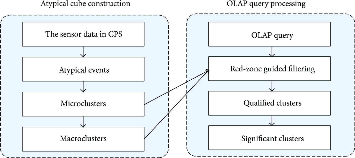
The overview of system framework.

Atypical Cube Construction

This component offline builds up the atypical cube from the sensor data in CPS. The system first retrieves the atypical events from the dataset and then constructs the atypical microcluster to store the features of each individual event. The similarity of micro-clusters is measured based on the retrieved features. The system merges similar micro-clusters as macroclusters to integrate multiple events. The clusters are formed in hierarchical trees to construct the atypical cube, which will be used to help process the OLAP queries.

OLAP Query Processing

This component online processes the OLAP query. The key issue is to efficiently retrieve significant clusters in the query range. The query processing algorithm first determines the possible regions where the significant clusters might be (i.e., red-zones) and then prunes the micro-clusters locating outside those regions. Only the qualified micro-clusters are selected to generate the macroclusters as query results. For the OLAP query in small range, the system utilizes a two-stage query processing technique: first returns an approximate answer in short time and then computes the detailed query results.

We will introduce the cube construction methods in Section 3 and query processing techniques in Section 4. Table 2 lists the notations used throughout this paper.

Table 2

List of notations.

Notation	Explanation	Notation	Explanation
R	The CPS dataset	$r_{i}$ , $r_{j}$	The atypical data records
S	The sensor set	$s_{1}$ , $s_{2}$	The sensors
T	The time period	$t_{1}$ , $t_{2}$	The time windows
SF	The spatial feature	TF	The temporal feature
$f (s, t)$	The severity measure	$F (S, T)$	The total severity
$E_{A}, E_{B}$	The atypical events	W	The spatial region
$Q (W, T)$	The analytical query	$C_{A}, C_{B}$	The atypical clusters
$μ_{i}$	The agg. severity by $s_{i}$	$ν_{i}$	The agg. severity by $t_{j}$
$δ_{t}$	The time threshold	$δ_{d}$	The distance threshold
$δ_{s}$	The severity threshold	$δ_{sim}$	The similarity threshold

3. Atypical Cube Construction

3.1. Bottom-up Styled Cube

Traditional methods construct the atypical cube by aggregating severity measures in a bottom-up style. The hierarchies are predefined on temporal, spatial, and other related dimensions, and the severities are then aggregated following such hierarchies. For example, the severity is aggregated by hour, day, month, and year in temporal dimension. In the spatial dimension, the hierarchies are built by partitioning the data with fixed regions, such as zipcode areas, street names [14], highway numbers [15], or the R-trees rectangles [16].

In this study, we employ a common measure of severity to describe the seriousness of atypical data in CPS. The severity function $f (w, t)$ is defined on the spatial and temporal domains, where w can be any region in a spatial coverage W and t can be any time of the temporal range T. Since the CPS sensors are usually fixed in their locations, with the help of a topology graph mapping the sensors to spatial regions, the region W is then represented by a sensor set S that for all $s \in S$ , s is located in W. Then the total severity can be computed on discrete sets as (1):

\begin{matrix} F (S, T) & = \sum_{s \in S}^{} \sum_{t \in T}^{} f (s, t) . \end{matrix}

(1)

Property 2.

The total severity $F (S, T)$ is a distributive measure.

Proof.

A measure is distributive if it can be derived from the aggregation values of n subsets, and the measure is the same as that derived from the entire data set [13].

Let us partition the dataset in S and T into n subsets, each with $S_{i} \subset S$ and $T_{i} \subset T$ . The severity of the $i th$ subset is computed by aggregating the severities of every subset as shown in the following:

F (S_{i}, T_{i}) = \sum_{s \in S_{i}} \sum_{t \in T_{i}} f (s, t) .

(2)

Then total severity is computed as

F (S, T) = \sum_{1}^{n} F (S_{i}, T_{i})

. Since

⋃_{i = 1, \dots, n}^{} S_{i} = S

and

⋃_{i = 1, \dots, n}^{} T_{i} = T

F (S, T) = \sum_{s \in S} \sum_{t \in T} f (s, t) .

(3)

Therefore

F (S, T)

is in the same format from the one derived from the entire dataset, and it is a distributive measure.

The distributive measure is efficient to compute [13], and the bottom-up styled approach is fast in both cube construction and query processing. However, the information of total severity is too abstract to answer the queries like “where and how do the traffic congestions start and expand?”

Example 6.

The bottom-up styled cube is constructed by zipcode areas. The regions with high total severity are tagged out as red zones, for example, $a, b, \dots, g$ in Figure 2. However the cube only points out where the congestions are. It does not give detailed information on when those congestions start and which part is the most serious in a specified red zone.

Figure 2

Problems of Bottom-up Styled Cube.

The bottom-up styled cube cannot provide details since the numeric measure of total severity is not enough to describe the complex atypical events. In addition, the atypical events may not follow predefined regions. The three major congestions A, B, and C in Figure 2 are partitioned into seven red zones by bottom-up styled cube. It is natural to lead users to illusions that the fragments of A and B congest together in area a. But a careful examination reveals that the highway segments A (freeway 10W) usually congest in the morning rush hours and the segments B (freeway 10E) jam in the evenings. They seldom congest together and should be distinguished from each other.

3.2. Basic Atypical Cluster

In real applications, the users usually cannot provide accurate boundaries to separate atypical events. Instead, the system is required to discover such boundaries automatically and distinguish different atypical events to the users. For this purpose, we propose the concept of basic atypical cluster.

Definition 7 (Basic Atypical Cluster).

Let E be an atypical event with sensor set $S = {s_{1}, s_{2}, \dots, s_{n}}$ and time window sequence $T = {t_{1}, t_{2}, \dots, t_{m}}$ ; the basic atypical cluster C of E is defined as $C = 〈 IF, SF, TF 〉$ , in which $IF$ is the identity features, such as cluster ID, date, street name, and highway numbers; the spatial feature $SF = {〈 s_{1}, μ_{1} 〉, 〈 s_{2}, μ_{2} 〉, \dots, 〈 s_{n}, μ_{n} 〉}$ , $μ_{i} = \sum_{T}^{} f (s_{i}, t)$ is the aggregated severity of sensor $s_{i}$ ; the temporal feature $TF = {〈 t_{1}, ν_{1} 〉, 〈 t_{2}, ν_{2} 〉, \dots, 〈 t_{m}, ν_{m} 〉}$ , $ν_{j} = \sum_{S}^{} f (s, t_{j})$ is the aggregated severity of time window $t_{j}$ .

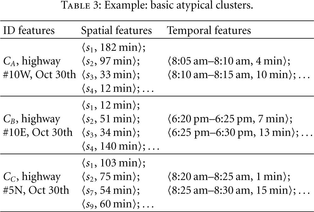
Intuitively speaking, the spatial feature is the summary of the atypical event in temporal dimension, and the temporal feature is the summary of the event in spatial dimension. $μ_{i}$ represents how long the sensor $s_{i}$ is atypical in E, and $ν_{j}$ reflects how many sensors are atypical during time window $t_{j}$ of E. In this way the basic atypical cluster C denotes the coverage, time length, and seriousness of corresponding atypical event.

Example 8.

Table 3 shows the basic atypical clusters retrieved from Example 6. The ID feature is a general description of the corresponding atypical event; for example, $C_{A}$ is generated from event $E_{A}$ which happens in highway 10W on October 30th. The spatial and temporal features are generated by aggregating the atypical records. Note that since the sensors may have different atypical durations in a time window, we still use the accumulated time duration to denote the number of atypical sensors in temporal features. The spatial and temporal features can be directly used to answer the queries in Example 1; for example, the congestion event A starts at around 8:05 am, and the most serious part is the road segment monitored by $s_{1}$ ; it experiences total 182 minutes of congestion in event $E_{A}$ .

Table 3

Example: basic atypical clusters.

ID features	Spatial features	Temporal features
$C_{A}$ , highway #10W, Oct 30th	$〈 s_{1}, 182 min 〉$ ; $〈 s_{2}, 97 min 〉$ ; $〈 s_{3}, 33 min 〉$ ; $〈 s_{4}, 12 min 〉$ ; …	$〈 8:05 am - 8:10 am, 4 min 〉$ ; $〈 8:10 am - 8:15 am, 10 min 〉$ ; …

$C_{B}$ , highway #10E, Oct 30th	$〈 s_{1}, 12 min 〉$ ; $〈 s_{2}, 51 min 〉$ ; $〈 s_{3}, 34 min 〉$ ; $〈 s_{4}, 140 min 〉$ ; …	$〈 6:20 pm - 6:25 pm, 7 min 〉$ ; $〈 6:25 pm - 6:30 pm, 13 min 〉$ ; …

$C_{C}$ , highway #5N, Oct 30th	$〈 s_{1}, 103 min 〉$ ; $〈 s_{2}, 75 min 〉$ ; $〈 s_{7}, 54 min 〉$ ; $〈 s_{9}, 60 min 〉$ ; …	$〈 8:20 am - 8:25 am, 1 min 〉$ ; $〈 8:25 am - 8:30 am, 15 min 〉$ ; …

The atypical events are retrieved by a single scan of the dataset, and the basic atypical clusters can be generated simultaneously. Algorithm 1 shows the detailed process.

Algorithm 1: Basic cluster generation.

Input: the time interval threshold $δ_{t}$ , distance threshold $δ_{d}$ , atypical

dataset R

Output: The basic atypical cluster set basic_set

1 repeat

2 randomly select a seed record r from R;

3 retrieve all the atypical connected records from r w.r.t. $δ_{t}$ and $δ_{d}$ ;

4 group those records to form an atypical event E(S; T);

5 initialize basic cluster $C 〈 IF; SF; TF 〉$ ;

6 foreach sensor $s_{i} \in S$ do

7 compute the sensor severity $μ_{i}$ ;

8 add $〈 s_{i}, μ_{i} 〉$ to $SF$ ;

9 end

10 foreach time window $t_{j}$ ∈ $T$ do

11 compute the time window severity $ν_{j}$ ;

12 add $〈 t_{j}, ν_{j} 〉$ to $TF$ ;

13 end

14 add C to basic_set;

15 $R \leftarrow R - E$

16 until $R = ϕ$ ;

17 return basic_set;

The basic cluster generation algorithm randomly picks a seed record from the dataset (Line 2) and retrieves all the atypical connected records to it (Line 3). Then the algorithm groups those records as an atypical event (Line 4) and generates the spatial and temporal features of basic cluster (Lines 6–13). Those steps are repeated until all the data are processed.

Proposition 9.

The time complexity of Algorithm 1 is $O (n^{2})$ without index and $O (n \cdot \log (n))$ with spatial index (e.g., R-tree), where n is the number of atypical records.

Proof.

The major cost of Algorithm 1 is on Line 3 to retrieve the atypical connected records. If there is no index on the temporal and spatial dimensions, it costs $O (n)$ time to retrieve the neighbors of one seed, and each atypical record's connected records are retrieved only once. Thus the entire step takes $O (n^{2})$ time. However the neighbor searching algorithm can speed up to $O (\log (n))$ with a spatial index such as R-tree, and hence the time complexity of the algorithm is improved as $O (n \cdot \log (n))$ .

3.3. Atypical Cluster Aggregation

The first task of cluster aggregation is to compute the similarities between two atypical clusters. The cluster similarity is measured based on both the spatial and temporal features, as shown in (4). Two clusters are considered similar to each other only when they have atypical records at the same places during the same time periods. Equations (5) and (6) show the calculation of spatial and temporal similarities, where $S_{i}$ is the sensor set, $T_{i}$ is the time window set, and $μ^{i}$ and $ν^{i}$ are the aggregated severity of sensor s and time window t in cluster $C_{i}$ , respectively. Equation (5) computes the severity percentages of common sensors over a cluster and balances the values on two clusters by a mathematical function $g (p_{1}, p_{2})$ . The function $g (p_{1}, p_{2})$ could be in the form of max, min, the arithmetic mean, harmonic mean, or geometric mean. The reason of using different mathematical balance function here is that the size of two clusters may be different. When comparing the similarity between a large cluster and a small one, the percentage of common sensors is inevitably small for the larger cluster. If we use the max function, the two clusters are still similar even if the common sensor percentage is low for the larger cluster:

\begin{gathered} Sim (C_{1}, C_{2}) = \frac{1}{2} (Si m_{SF} (C_{1}, C_{2}) + Si m_{TF} (C_{1}, C_{2})) \end{gathered},

(4)

\begin{matrix} Si m_{SF} (C_{1}, C_{2}) = g (\frac{\sum_{S_{1} \cap S_{2}}^{} μ^{1}}{\sum_{S_{1}}^{} μ^{1}}, \frac{\sum_{S_{1} \cap S_{2}}^{} μ^{2}}{\sum_{S_{2}}^{} μ^{2}}), \end{matrix}

(5)

\begin{gathered} Si m_{TF} (C_{1}, C_{2}) = g (\frac{\sum_{T_{1} \cap T_{2}}^{} ν^{1}}{\sum_{T_{1}}^{} ν^{1}}, \frac{\sum_{T_{1} \cap T_{2}}^{} ν^{2}}{\sum_{T_{2}}^{} ν^{2}}) . \end{gathered}

(6)

Once two micro-clusters are merged, a single macro-cluster is created to represent the result out of this merge (here we use the term micro-cluster to denote the merge input and macro-cluster to denote the merge result). The spatial feature of the macro-cluster is calculated as shown in (7): the system accumulates the severities of common sensors from two micro-clusters and keeps the nonoverlapping ones; so is the temporal feature. A new ID is generated for the macro-cluster:

\begin{matrix} S F_{new} & = {〈 s_{i}, μ_{i}^{1} + μ_{i}^{2} 〉 | s_{i} \in (S_{1} \cap S_{2})} \\ \cup {〈 s_{j}, μ_{j} 〉 | s_{j} \notin (S_{1} \cap S_{2}), s_{j} \in (S_{1} \cup S_{2})} . \end{matrix}

(7)

Property 3.

The spatial and temporal features in atypical clusters are algebraic measures.

Proof.

A measure is algebraic if it can be computed by an algebraic function with m arguments (m is a bounded positive integer), and each of the arguments is distributive [13]. We will prove that the spatial feature is algebraic in the process of integrating n micro-clusters to a macro-cluster by mathematical induction.

(1) The Basis. First we study the case that $n = 2$ .

Let $S_{1}$ and $S_{2}$ be the sensor sets of two micro-clusters; the spatial feature of macro-cluster $S F_{macro}$ is computed as (8):

\begin{matrix} S F_{macro} & = {〈 s_{i}, μ_{i}^{1} + μ_{i}^{2} 〉 | s_{i} \in (S_{1} \cap S_{2})} \\ \cup {〈 s_{j}, μ_{j} 〉 | s_{j} \notin (S_{1} \cap S_{2}), s_{j} \in (S_{1} \cup S_{2})} . \end{matrix}

(8)

The sensor severity μ is a distributive measure, according to the definition, and spatial feature is algebraic when

n = 2

(2) The Inductive Step. Suppose that the statement holds for $n - 1$ ; we study the case of integrating n micro-clusters.

The macro-cluster $C_{N}$ can be seen as the integration of the macro-cluster $C_{N - 1}$ and the $n th$ micro-cluster $C_{n}$ . Let $S_{N - 1}$ and $S_{n}$ be the corresponding sensor sets; the spatial feature of macro-cluster $S F_{N}$ is computed as (9):

\begin{matrix} S F_{N} & = {〈 s_{i}, μ_{i}^{1} + μ_{i}^{2} 〉 | s_{i} \in (S_{N - 1} \cap S_{n})} \\ \cup {〈 s_{j}, μ_{j} 〉 | s_{j} \notin (S_{N - 1} \cap S_{n}), s_{j} \in (S_{N - 1} \cup S_{n})} . \end{matrix}

(9)

Therefore the statement holds for case of integrating n micro-clusters. The spatial feature is algebraic.

From the same steps, it is easy to obtain that the temporal feature is also algebraic.

The algebraic measures are also efficient to compute and aggregate [13]; thus we use atypical clusters as the measure in atypical cube. The detailed micro-cluster merging steps are shown in Algorithm 2. The system accumulates the severity of common sensors in two micro-clusters (Lines 2–6) and copies the nonoverlapping ones (Line 7); the same steps are carried out in temporal features (Lines 9–16).

Algorithm 2: Merge Micro-Clusters.

Input: micro-clusters $C_{1} 〈 I F_{1}, S F_{1},T F_{1} 〉$ and $C_{2} 〈 I F_{2}, S F_{2},T F_{2} 〉$

Output: macro-cluster $C_{new} 〈 I F_{new}, S F_{new}, T F_{new} 〉$

1 foreach sensor $s_{i}$ ∈ $S F_{1}$ do

2 if $s_{i}$ ∈ $S F_{2}$ then

3 $μ_{i}^{new} = μ_{i}^{1} + μ_{i}^{2}$ ;

4 add $〈 s_{i}, μ_{i}^{new} 〉$ to $S F_{new}$ ;

5 remove the records of $s_{i}$ from $S F_{1}$ and $S F_{2}$ ;

6 end

7 add the rest records of $S F_{1}$ , $S F_{2}$ to $S F_{new}$

8 end

9 foreach time window $t_{j}$ ∈ $T F_{1}$ do

10 if $t_{j}$ ∈ $T F_{2}$ then

11 $ν_{j}^{new} = ν_{j}^{1} + ν_{j}^{2}$ ;

12 add $〈 s_{j}, μ_{j}^{new} 〉$ to $T F_{new}$ ;

13 remove the records of $t_{j}$ from $T F_{1}$ and $T F_{2}$ ;

14 end

15 add the rest records of $T F_{1}$ , $T F_{2}$ to $T F_{new};$

16 end

17 generate $I F_{new}$ ;

18 return $C_{new}$ ;

Property 4.

The operation of merging atypical clusters is mathematically commutative and associative.

Proof.

To prove that the merge operation is mathematically commutative, we have to show that for any $C_{1}$ and $C_{2}$ , $C_{1}$ merge $C_{2}$ = $C_{2}$ merge $C_{1}$ .

For two clusters 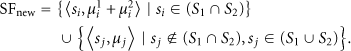$C_{1}$ and $C_{2}$ , the spatial feature of their integrating cluster is $S F_{new}$ computed as

\begin{matrix} S F_{new} & = {〈 s_{i}, μ_{i}^{1} + μ_{i}^{2} 〉 | s_{i} \in (S_{1} \cap S_{2})} \\ \cup {〈 s_{j}, μ_{j} 〉 | s_{j} \notin (S_{1} \cap S_{2}), s_{j} \in (S_{1} \cup S_{2})} . \end{matrix}

(10)

The positions of $S_{1}$ and $S_{2}$ are equal in the above equation; $S F_{new}$ is not influenced by the order of $C_{1}$ and $C_{2}$ . It is the same for temporal feature computation. And the identity feature is generated independently. Therefore for any $C_{1}$ and $C_{2}$ , $C_{1}$ merge $C_{2}$ = $C_{2}$ merge $C_{1}$ . The merge operation is mathematical commutative.

To prove that the merge operation is mathematically associative, we have to show that for any $C_{1}$ , $C_{2}$ and $C_{3}$ , ( $C_{1}$ merge $C_{2}$ ) merge $C_{3}$ = $C_{1}$ merge ( $C_{2}$ merge $C_{3}$ ).

Let us denote the following:

$C_{4}$ = $C_{1}$ merge $C_{2}$ ; $C_{5}$ = $C_{2}$ merge $C_{3}$ ;

$C_{6}$ = $C_{4}$ merge $C_{3}$ = ( $C_{1}$ merge $C_{2}$ ) merge $C_{3}$ ;

$C_{7}$ = $C_{1}$ merge $C_{5}$ = $C_{1}$ merge $(C_{2} merge C_{3})$ .

The spatial feature $SF (C_{6})$ is computed as

\begin{matrix} SF (C_{6}) & = {〈 s_{i}, μ_{i}^{4} + μ_{i}^{3} 〉 | s_{i} \in (S_{4} \cap S_{3})} \\ \cup {〈 s_{i}, μ_{i} 〉 | s_{i} \notin (S_{4} \cap S_{3}), s_{i} \in (S_{4} \cup S_{3})} . \end{matrix}

(11)

Since $S_{4} = S_{1} \cup S_{2}$ , (11) can be written as

\begin{matrix} SF (C_{6}) & = {〈 s_{i}, μ_{i}^{1,2} + μ_{i}^{3} 〉 | s_{i} \in ((S_{1} \cup S_{2}) \cap S_{3})} \\ \cup {〈 s_{i}, μ_{i} 〉 | s_{i} \notin ((S_{1} \cup S_{2}) \cap S_{3}), \\ s_{i} \in ((S_{1} \cup S_{2}) \cup S_{3})} \\ = {〈 s_{i}, μ_{i}^{1} + μ_{i}^{2} + μ_{i}^{3} 〉 | s_{i} \in (S_{1} \cap S_{2} \cap S_{3})} \\ \cup {〈 s_{i}, μ_{i}^{1} + μ_{i}^{3} 〉 | s_{i} \in (S_{1} \cap S_{3}), s_{i} \notin S_{2}} \\ \cup {〈 s_{i}, μ_{i}^{2} + μ_{i}^{3} 〉 | s_{i} \in (S_{2} \cap S_{3}), s_{i} \notin S_{1}} \\ \cup {〈 s_{i}, μ_{i}^{1} + μ_{i}^{2} 〉 | s_{i} \in (S_{1} \cap S_{2}), s_{i} \notin S_{3}} \\ \cup {〈 s_{i}, μ_{i} 〉 | s_{i} \in (S_{1} \cup S_{2} \cup S_{3}), \\ s_{i} \notin (S_{1} \cap S_{3}), s_{i} \notin (S_{2} \cap S_{3}), s_{i} \notin (S_{1} \cap S_{2})} . \end{matrix}

(12)

Since $S_{5} = S_{2} \cup S_{3}$ , (12) can be converted to

\begin{matrix} SF (C_{6}) & = {〈 s_{i}, μ_{i}^{1} + μ_{i}^{2,3} 〉 | s_{i} \in (S_{1} \cap (S_{2} \cup S_{3}))} \\ \cup {〈 s_{i}, μ_{i} 〉 | s_{i} \notin (S_{1} \cap (S_{2} \cup S_{3})), \\ s_{i} \in (S_{1} \cup (S_{2} \cup S_{3}))} \\ = {〈 s_{i}, μ_{i}^{1} + μ_{i}^{5} 〉 | s_{i} \in (S_{1} \cap S_{5})} \\ \cup {〈 s_{i}, μ_{i} 〉 | s_{i} \notin (S_{1} \cap S_{5}), s_{i} \in (S_{1} \cup S_{5})} \\ = SF (C_{7}) . \end{matrix}

(13)

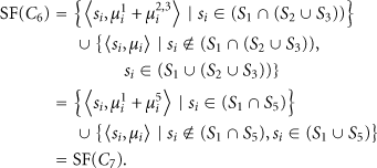
Equation (13) shows that the spatial features are the same for the macroclusters $C_{6}$ and $C_{7}$ , so are the temporal features. And the identity feature is generated independently. Hence the merge operation is mathematical associative.

Property 4 tells us that the order of micro-clusters does not influence the macro-cluster results. Thus we design the aggregation clustering process as Algorithm 3. The algorithm starts by checking each pair of the micro-clusters. If their similarity is larger than the given threshold, a merge operation is called to integrate them (Lines 2–4). This process is irrelevant to the order of micro-clusters. The new cluster is put back to the set, and the old pair is discarded (Lines 5–6). The program stops until no clusters could be merged (Line 9).

Algorithm 3: Aggregation clustering.

Input: micro-cluster set micro_set from lower cells, similarity

threshold $δ_{sim}$

Output: the macro-cluster set macro_set

1 repeat

2 foreach micro-cluster pair $C_{i}, C_{j}$ do

3 if Sim $(C_{i}, C_{j}) > δ_{sim}$ then

4 $C_{new}$ = merge $(C_{i}, C_{j})$ ;

5 add $C_{new}$ to micro_set;

6 remove $C_{i}$ , $C_{j}$ from micro_set;

7 end

8 end

9 until no clusters can be merged in micro_set;

10 macro_set ← micro_set;

11 return macro_set;

Proposition 10.

Let m be the number of micro-clusters; the time complexity of Algorithm 3 is $O (m^{2})$ .

Proof.

In the worst case, there are no similar pairs that can be found to be merged together. Then the algorithm needs to check the similarity between every pair and the total calculation times are $m (m - 1) / 2$ . Hence the time complexity of Algorithm 3 is $O (m^{2})$ .

Note that the similarity threshold $δ_{sim}$ is an important parameter for Algorithm 3. $δ_{sim}$ should be set larger than 0.5, since the clusters should be both spatially close and temporally related. On the other hand, if $δ_{sim}$ is too high (e.g., $δ_{sim} = 1$ ), no atypical cluster will merge with other ones and the macroclusters with high severity cannot be generated. We have conducted a performance study in Section 5.3; the experiment results suggest that the algorithm has the best performance if $δ_{sim}$ is set around 0.6.

Example 11.

Table 3 lists three atypical clusters, namely, $C_{A}$ , $C_{B}$ , and $C_{C}$ . Suppose that $δ_{sim}$ is set as 0.6. The aggregation clustering algorithm first checks the cluster pair of $C_{A}$ and $C_{B}$ and computes their similarity. Since they are only spatially close but not timely related, $Sim (C_{A}, C_{B}) = 0.49$ , which is less than $δ_{sim}$ . Hence this pair will not be integrated in one cluster. Then, the system picks the pair of $C_{A}$ and $C_{C}$ , since these two clusters have most of their atypical data in the common areas with similar times, $Sim (C_{A}, C_{C}) = 0.87$ ; thus they should be merged according to (4). The merged result is tagged as cluster $C_{D}$ . And the similarity between $C_{B}$ and $C_{D}$ is still lower than $δ_{sim}$ . The aggregation clustering algorithm stops and outputs $C_{B}$ and $C_{D}$ as the results.

The aggregation clustering algorithm takes the micro-clusters from children cells as input and outputs the macroclusters to store as measures in the parent cell. Such macroclusters are also going to be used as new inputs to get even higher-level clusters. In this way a hierarchical clustering tree is built up.

The atypical cube is constructed as a forest of hierarchical clustering trees, where each tree represents an aggregation path in the cube. Figure 3 shows the framework of atypical cube for the case of traffic congestions. Ten basic atypical clusters are stored in the lowest-level cells. The aggregation cells $b_{1}, \dots, b_{6}$ are built on them, and the apex cell $a_{1}$ has two macroclusters integrated from the micro-clusters in $b_{1}, \dots, b_{6}$ .

Figure 3

Example: the framework of atypical cube.

4. OLAP Query Processing

4.1. Processing Large-Scale Queries

In practical applications we do not precompute the entire atypical cube due to storage limits. In most cases only the basic clusters and some low-level micro-clusters are precomputed. With such a partially materialized data structure, the system needs to dynamically integrate the low-level clusters to process OLAP queries in large query range. The online clustering process is similar to the cluster integration algorithm. However there are two problems. (1) The first one is efficiency: the time complexity of cluster aggregation algorithm is quadratic to the number of input clusters. Therefore the system should select only the relevant micro-clusters to reduce the time cost. (2) The second is effectiveness: if the query scale is large, for example, the users want the monthly congestion report of the whole city. There may be a large number of macroclusters in the query range, but only few of them are significant clusters with high severities, while the others are negligible. When constructing atypical cube, the process is offline and the system can store all the clustering results. When processing online queries, the users usually demand the significant clusters being delivered in short time and do not prefer the results mixed with trivial clusters.

Definition 12 (Significant Cluster).

Let $Q (W, T)$ be a query with the range in region W and time T. The cluster C is significant if $severity (C) > δ_{s} \cdot length (T) \cdot N$ , where $δ_{s}$ is the severity threshold and N is the number of sensors in W and $severity (C) = \sum_{SF}^{} μ_{i} = \sum_{TF}^{} ν_{j}$ .

Note that the system measures the cluster significance by a relative threshold $δ_{s}$ , because $severity (C)$ is influenced by the query scales; for example, the severities of high-level clusters in one month are usually larger than the low-level clusters in a day.

The key challenge for online clustering is to prune the trivial micro-clusters and meanwhile guarantee the accuracy of significant macroclusters. One strategy is beforehand pruning: the system pushes down the prune step to lower levels by only selecting the significant micro-clusters for integration. However this strategy cannot guarantee finding all the significant macroclusters, because a micro-cluster that contributes to a significant macro-cluster may not be significant by itself. If the algorithm prunes all insignificant micro-clusters beforehand, the severity of the macro-cluster will also be reduced and may not be significant anymore.

Example 13.

The micro-clusters of Los Angeles in October 30th are shown in Figure 4(a), and the monthly significant macroclusters A and B are plotted in Figure 4(b). In Figure 4(a), the micro-clusters a, b, j, k, and o are going to be integrated as parts of the significant macroclusters even if they are relatively trivial. The micro-clusters e, h, and i are significant in the scale of one day, but actually they can be pruned since they have no contribution for any significant macroclusters in one month.

Figure 4

Example: problem of beforehand pruning.

Can We Foretell Which Microcluster Will Become a Part of the Significant Macroclusters and Which Will Not? If the system knows such guiding information, it can improve query efficiency and meanwhile guarantee the result's accuracy. The heuristic comes from the bottom-up method: recall that the bottom-up method uses total severity $F (S, T)$ as the measure. As a distributive measure, $F (S, T)$ is efficient to compute [13] and can be employed as the guidance to retrieve significant clusters.

One may worry that $F (S, T)$ is computed on predefined regions such as zipcode areas, and their boundaries are different from the atypical clusters. Fortunately, Property 5 shows that there is a relation between predefined regions and atypical clusters.

Property 5.

Let $Q (W, T)$ be an OLAP query, let $δ_{s}$ be the relative severity threshold, let $W^{'}$ be a spatial region that $W^{'} \subseteq W, and let S^{'}$ and S be the sensor sets installed in regions $W^{'}$ and W, respectively. If $F (S^{'}, T) < δ_{s} \cdot Length (T) \cdot | S |$ , then there is no significant macro-cluster in $S^{'}$ within time T.

Proof.

We will prove the statement by contradiction.

Suppose that there is a cluster $C_{j}$ with sensor set $S_{j} \subseteq S'$ and time window sequence $T_{j} \subseteq T$ , such that $Severity (C_{j}) \geq δ_{s} \cdot Length (T) \cdot | S |$ .

Since $F (S^{'}, T)$ is the aggregation of total severity in $S'$ and T,

F (S^{'}, T) \geq Severity (C_{j}) \geq δ_{s} \cdot Length (T) \cdot | S | .

(14)

We now have a contradiction with the condition that $F (S^{'}, T) < δ_{s} \cdot Length (T) \cdot | S |$ . Hence there does not exist such cluster $C_{j}$ .

Property 5 can be used to help filtering the micro-clusters. The system only needs to integrate the clusters in the regions where the total severities are larger than threshold, that is, the red zones.

Example 14.

In Figure 5, the red zones are tagged out. They are generated by the bottom-up styled cube with a predefined zipcode area hierarchy. The micro-clusters e, g, i, and m can be pruned safely since they are outside the zones; a, b, and d should be kept for clustering since they are in the zones; c, k, f, o, and n are also kept since they intersect with the red zones and may contribute to macroclusters.

Figure 5

Red-zone guided clustering.

Algorithm 4 shows detailed steps of red zone guided online clustering. The system first computes the severity on predefined regions in bottom-up styled cube and retrieves the red zones (Lines 1–4) and then selects out the micro-clusters in red zones (Lines 5–7). The clustering algorithm (Algorithm 1) is called to generate the macroclusters (Line 8). Since the algorithm can only guarantee there are no false negatives (i.e., not missing any significant macroclusters), it is possible to generate some false positives. A check procedure is processed to prune the clusters without enough severity at the last step (Lines 9–11).

Algorithm 4: Red-zone guided clustering.

Input: query $Q (S, T)$ , micro-cluster set $m i c r o_s e t$ from materialized

children cells, bottom-up style cube $b u_c u b e,$ similarity

threshold $δ_{sim}$ , relative severity threshold $δ_{s}$

Output: the significant macro-cluster set sig_set for the query

1 Compute $F (S_{i}, T)$ from bu_cube for $Q (S, T)$ ;

2 If $F (S_{i}, T) \geq δ_{s} \cdot Length (T) \cdot | S | then$

3 add $S_{i}$ to red zone set red_set;

4 end

5 foreach micro-cluster $C_{i} \in m i c r o_s e t$ do

6 if $C_{i} \in r e d_s e t o r C_{i}$ intersects with red_set then add $C_{i}$ to

7 $s i g_m i c r o_s e t$ ;

7 end

8 $s i g_s e t \leftarrow$ clustering $(s i g_m i c r o_s e t, δ_{sim})$ (Algorithm 1)

9 foreach $c l u s t e r C_{i} \in s i g_s e t$ do

10 if $Severity (C_{i}) < δ_{s} \cdot Length (T) \cdot | S |$ then remove $C_{i}$ ;

11 end

12 return $s i g_s e t$ ;

The major cost of Algorithm 4 is at Line 8 to call the clustering algorithm. In the worst case, no cluster could be filtered out, and the algorithm's time complexity is still quadratic to the number of micro-clusters. However, in our experiments, about 80% micro-clusters could be filtered out with reasonable $δ_{s}$ , and the query efficiency was improved dramatically.

4.2. Drill-Through Query Processing

In some rare cases, the users require detailed results in a very narrow range, such as “what is the congestion details from 8:45 am to 9 am of the highway #101 near downtown?” The system needs to decompose basic atypical clusters to answer them. Such queries actually drill through the atypical cube to the original sensor dataset.

We propose a two-stage algorithm to process this kind of queries. The system first returns the related basic atypical clusters as an approximate result and then decomposes them for precise answers. The details are shown in Algorithm 5 as a two-stage process: in the first stage, the system retrieves all related micro-clusters, directly integrates them and returns the macroclusters as approximate result (Lines 1–5); then it drills through to the sensor dataset and refines those micro-clusters in the second stage (Lines 6–12). The precise results are computed and returned later.

Algorithm 5: Drill-through query processing.

Input: atypical cube $c u b e$ , drill-through query Q, similarity threshold

$δ_{sim}$

Output: The approximate result $R_{a}$ , the precise result $R_{p}$

1 foreach basic atypical cluster $C_{i}$ in cube do

2 if $C_{i}$ related to Q then add $C_{i}$ to micro_set;

3 end

4 $R_{a}$ ← clustering $(m i c r o_s e t, δ_{sim})$ (Algorithm 1);

5 return $R_{a}$ ;

6 foreach $C_{i}$ do

7 drill through to the sensor dataset;

8 $C_{i}^{'}$ ← filter the records in $C_{i}$ with Q's condition;

9 add $C_{i}^{'}$ to $m i c r o_s e t'$ ;

10 end

11 $R_{p}$ ← clustering $(m i c r o_s e t', δ_{sim})$ ;

12 return $R_{p}$ ;

Since the query range is narrow, the size of the $m i c r o_s e t$ is usually small; the major cost of Algorithm 5 is in the drill-through step with high I/O overhead (Line 7). However if the system builds an index for the atypical events in the sensor data and maintains an inverted pointer p from each basic atypical cluster to the corresponding atypical events, the time cost of Algorithm 5 will be improved significantly.

5. Performance Evaluation

Since the idea of this study is motivated by practical application problems, we use real world datasets to evaluate the proposed approaches. Twelve datasets are collected from the PeMS traffic monitoring system [11]; each stores one-month traffic data in the areas of Los Angeles and Ventura. The data are collected from over 4,000 sensors on 38 highways. There are more than 1.1 million records for a single day and totally 428 million records for the whole year. The total size of all the datasets is over 54 GB.

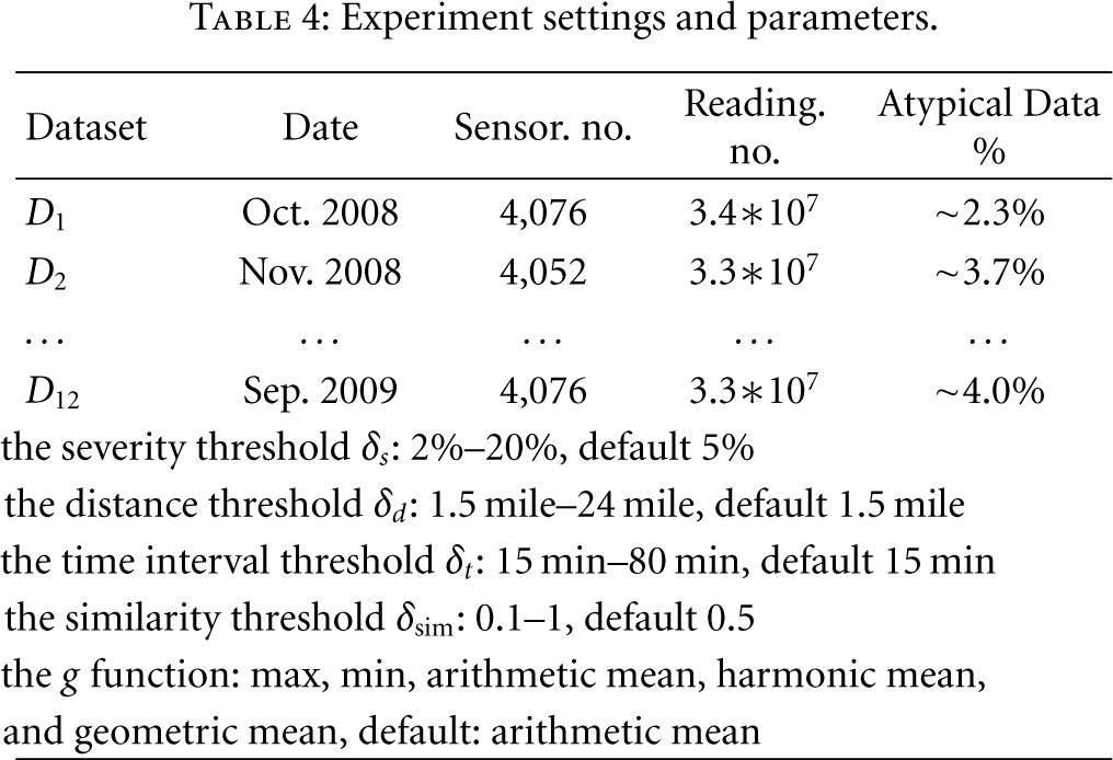
The experiments are conducted on a PC with an Intel 2200 Dual CPU at 2.20 G Hz and 2.19 G Hz. The RAM is 1.98 GB, and the operating system is Windows XP SP2. All the algorithms are implemented in Java on Eclipse 3.3.1 platform with JDK 1.5.0. The detailed experimental settings and parameters are listed in Table 4.

Table 4

Experiment settings and parameters.

Dataset	Date	Sensor. no.	Reading. no.	Atypical Data %
$D_{1}$	Oct. 2008	4,076	3.4*10⁷	~2.3%
$D_{2}$	Nov. 2008	4,052	3.3*10⁷	~3.7%
…	…	…	…	…
$D_{12}$	Sep. 2009	4,076	3.3*10⁷	~4.0%
the severity threshold $δ_{s}$ : 2%–20%, default 5%
the distance threshold $δ_{d}$ : 1.5 mile–24 mile, default 1.5 mile
the time interval threshold $δ_{t}$ : 15 min–80 min, default 15 min
the similarity threshold $δ_{sim}$ : 0.1–1, default 0.5
the g function: max, min, arithmetic mean, harmonic mean,
and geometric mean, default: arithmetic mean

5.1. Evaluations of Cube Construction

In this subsection we evaluate the algorithms of offline cube construction. CubeView [14] is a bottom-up method on traffic data. The original CubeView algorithm aggregates all the traffic records with predefined spatial and temporal hierarchies. In this experiment, the system carries out a preprocessing step to select atypical records and adjusts CubeView to construct the cube only on the atypical data. We first construct the cubes on a single dataset, then gradually increase the number of datasets, until all the twelve datasets are used in the experiment. Figure 6 shows the time costs of the original Cubeview (OC), modified CubeView (MC), the preprocessing step (PR), and our atypical-cluster-based method (AC). The x-axis is the number of datasets used in the experiment, and y-axis is the time cost of the algorithms. MC and AC are an order of magnitude faster than OC because they are constructed on the atypical data, which are only 2% to 5% of the original datasets. The time cost of PR is close to OC since both of them have to scan the original datasets with huge I/O overhead. However the preprocessing step only needs to carry out once for constructing different cubes.

Figure 6

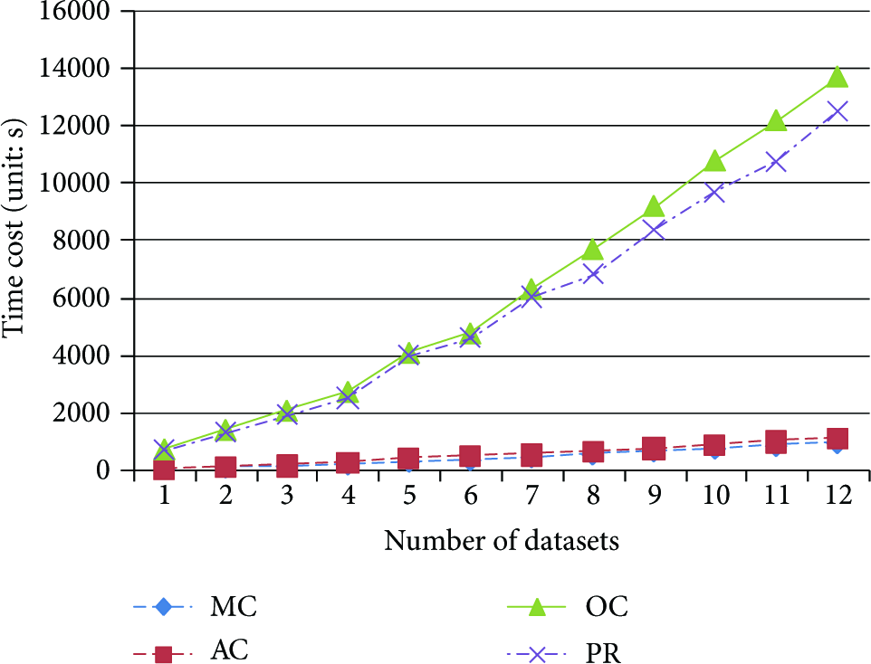
Efficiency: construction time cost versus no. of datasets.

Figure 7 shows the constructed cube size of original Cubeview (OC), modified CubeView (MC), and atypical cluster method (AC). The size of corresponding atypical events (AEs) is also recorded in the figure. MC achieves the best compression effects since it only records the numeric measure of total severity, but it cannot describe the complex atypical events. AC stores all the critical information about spatial and temporal features of AE, but only costs 0.5% to 1% space of AE.

Figure 7

Size: constructed cube size versus no. of datasets.

Figure 8(a) records the constructed cube size of the three methods on six different datasets. In general, the construction overhead and storage size of OC are acceptable since the cube is built offline. However, the results in Figure 8(b) show that OC cannot be used to process queries about atypical events. The average speeds of OC on all the datasets are all around 65 mph, which are close to the speed limit of California highway. The information is hence not interesting to the users since the atypical events are dwarfed by the majorities of normal data.

Figure 8

Results: cube size and avg. speed.

5.2. Comparisons in OLAP Query Processing

In this subsection we evaluate the performances of OLAP query processing. Three query processing strategies are compared: (1) integrating all the micro-clusters (All); (2) pruning the insignificant clusters beforehand (Pru); (3) the red-zone guided clustering (Gui).

In the experiments, the system only precomputes the micro-clusters of each day. The analytical query's spatial range is fixed as Los Angeles, and time range gradually increases from one week (requiring to aggregate the micro-clusters of 7 days) to three months (84 days). Figures 9(a) and 9(b) record the average time and I/O costs (measured by the number of input micro-clusters). Although Gui has extra cost to compute the redzones, the time efficiency is still close to Pru. From the figure one can see clearly that Gui and Pru are much more efficient than All. Gui's time cost is only about 15%–20% of All.

Figure 9

Efficiency: query time and I/O costs.

To evaluate the effectiveness of query results, we compute the precision and recall of the significant clusters. Since the integrating-all method prunes no clusters, its results contain all the significant clusters. The system checks the results of All and retrieves the true significant clusters as the ground truth. The measures of precision and recall are then computed as follows.

Precision

The precision is calculated as the proportion of significant clusters in the returned query results.

Recall

The recall is the proportion of retrieved significant clusters over the ground truth.

The system increases the query time range from 7 days to 84 days and records the precision and recall of three methods in Figure 10. For all the methods, their precision decreases with larger query range, because the cluster severity does not grow linearly with respect to the query range, and the significant clusters are inevitably fewer in larger query range with fixed severity threshold. In the experiment, Pru has the highest precision, because it prunes all the trivial micro-clusters and generates fewer macroclusters (Figure 10(a)). However, as shown in Figure 10(b), Pru cannot guarantee to find all the significant clusters. Its recall might even be lower than 50% in some cases. Therefore, even if Pru is the winner on efficiency and precision, it is not feasible to process analytical query since the significant clusters may be missed in the results.

Figure 10

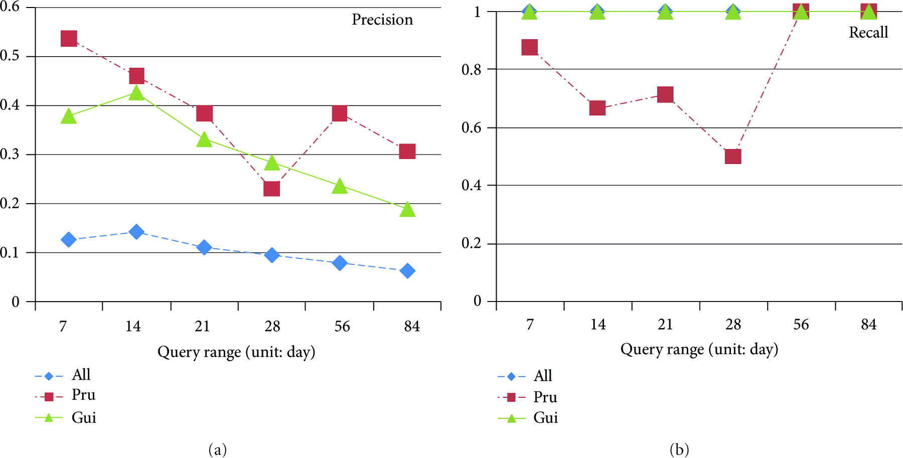
Effectiveness: precision and recall with respect to query range.

In the next experiment, we fix the query time range as 14 days and evaluate the influence of severity threshold $δ_{s}$ . The experimental results are shown in Figure 11. The precision drops with larger $δ_{s}$ , because fewer macroclusters can meet the high standard of severity to become significant. Another interesting observation is that the recall of Pru increases when $δ_{s}$ grows. Pru is unlikely to miss the macroclusters with very high severities. However, the detailed spatial and temporal features of those clusters may not be accurate, because Pru filters out some micro-clusters that should be integrated in.

Figure 11

Effectiveness: precision and recall with respect to $δ_{s}$ .

The precision of Gui in the above experiments is not high; however this measure can be easily improved. The system can efficiently filter out the false positives and guarantee 100% precision by checking the macro-cluster's total severity. Gui has such a procedure (Lines 5–7 in Algorithm 4). This procedure is turned off in the experiments for a fair play.

5.3. Parameter Tuning for Atypical Cluster Method

In the next experiment, we study the influence of the parameters in the atypical-cluster-based method, including time interval threshold $δ_{t}$ , distance threshold $δ_{d}$ , similarity threshold $δ_{sim}$ , and balance function g. The system first retrieves the micro-clusters in each day with different $δ_{t}$ and $δ_{d}$ and then carries out the cluster integration to generate the macroclusters for every week and month. Figure 12(a) shows the average number of the atypical clusters in every day, week, and month. The figure also records the average number of weekly/monthly significant clusters as sig(week)/sig(month). One can clearly see that the numbers of weekly and monthly macroclusters are much larger than the micro-clusters, but most of them are the trivial ones. Only 0.1% to 0.5% of those macroclusters are significant. When $δ_{t}$ increases, more clusters can be merged together and the numbers of macroclusters decrease rapidly. But the numbers of significant macroclusters are more stable. Since those significant clusters have already integrated a large amount of micro-clusters, they can hardly merge with each other due to large difference on spatial and temporal features. In Figure 12(b) we record the numbers of atypical clusters with different $δ_{d}$ . The influence of $δ_{d}$ is smaller than $δ_{t}$ . The number of significant cluster is also robust to this parameter.

Figure 12

Size: no. of clusters versus $δ_{t}$ and $δ_{d}$ .

We also study the influences of similarity threshold $δ_{sim}$ and the balance function g in (5) and (6). Since they only influence the cluster integration results, we carry out the integration process with various balance functions, including max, min, the arithmetic mean (avg), the geometric mean (geo) and harmony mean (har). Figure 13 shows the average severity of the significant clusters with respect to $δ_{sim}$ . Generally speaking, the max function integrates more clusters, and the min function is the most conservative. The differences among avg, geo, and har are minor. Hence we suggest that the users may choose a mean function (e.g., avg) as the balance function g.

Figure 13

Average severity of significant cluster versus $δ_{sim}$ .

From Figures 12 and 13, we can also learn that the result of significant cluster is robust to the time interval threshold $δ_{t}$ and distance threshold $δ_{d}$ , but the severity of significant clusters may reduce rapidly with larger similarity threshold $δ_{sim}$ . The reason is that no atypical cluster is totally the same with another one. If $δ_{sim}$ is too high, the micro-clusters cannot be merged and no significant clusters can be generated. In addition, $δ_{sim}$ should be set larger than 0.5, since the clusters that merged together must be both spatially close and temporally related. Based on the experiment results, we suggest setting $δ_{sim}$ around 0.6; in such way the aggregation clustering algorithm generates a few significant clusters with high severities.

5.4. Drill-Through Query Processing

At last we test the performances of drill-through query processing methods. In this experiment, the spatial range is no longer fixed to Los Angeles; instead it is set to a very narrow range of random road segments. In this way, the system has to drill through the basic atypical clusters to the original sensor dataset.

Since the algorithm is a two-stage process, we evaluate both stages separately in the experiments. We also compare the drill-through stage with indexes and the one without. Figure 14 shows their time costs w.r.t. the number of involved cells. Note that the axis of query time is in logarithmic scale. It is clear that the first stage of approximate query is much faster than the second stage of precise query. In drill-through queries, the I/O overhead is the dominant factor. The stage 1 of approximate query does not access to the detailed sensor data, so it is very efficient, and the results are returned to the users in less than ten seconds.

Figure 14

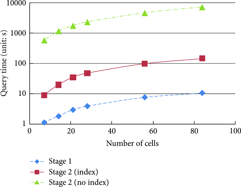
Efficiency: different stages of drill-through queries.

6. Extensions and Discussions

In this study, we illustrate the atypical cluster techniques mainly on spatial-temporal dimensions and carry out the performance evaluation on the sensor data in traffic system, because (1) the spatial and temporal dimensions are actually the most basic and important dimensions in many CPS applications, and the user's queries are usually related to such two dimensions; (2) large volume of sensor data in traffic applications is open to public; (3) the atypical events of traffic (i.e., the congestions) are actually more complex than in many other domains. Apart from spatial and temporal dimensions, the users may require to analyze the data on other domain specific dimensions. For example, in the traffic system, the transportation officer may want to check the congestions related to bad weather or the accident reports. The proposed framework can be easily extended to support the analysis on such context dimensions. The weather dimension can be joined with temporal dimension with the date, and the accident dimension can be joined with temporal and spatial dimensions by the accident time and location. Figure 15 shows a snowflake schema of the atypical cube with dimensions of temporal, spatial, weather, accident, and so on.

Figure 15

Atypical cube schema for congestions.

By joining those dimension tables, the system can support OLAP queries on more dimensions. For instance, if users want congestion reports related to traffic accidents, the system will first select out the region $W^{'}$ and time window set $T^{'}$ related to those accidents, then process query $Q (W^{'}, T^{'})$ by the red-zone guided clustering algorithm to get the results.

In the cube construction component, the major time cost is on the preprocessing step, since the system has to scan the original datasets with huge I/O overhead. However, the preprocessing step only needs to carry out once for constructing different cubes. The massive data can also be pre-processed by the sensors themselves in a distributed manner [17]. In such a way, the amount of data and events can be reduced. Due to the hardware limitations, the sensors are likely to report some error messages and untrustworthy atypical data may be generated then. Since the main theme of this study is on multidimensional analysis of atypical data, we assume that the clean and trustworthy records can be retrieved by CPS. In our previous studies, we have proposed several methods to retrieve the atypical events from untrustworthy sensors and carry out trustworthiness analysis for the sensor networks. More details can be found in [3, 18].

The clustering and integration methods used in this study are all “hard-clustering”; that is, a micro-cluster could only be merged to one macro-cluster. Hence it is possible that the clustering result may not be deterministic. However, the influence is limited for the analytical query, because the macroclusters are usually aggregated from hundreds of micro-clusters, and there is almost no difference on merging a single micro-cluster or not.

7. Related Works

According to the methodologies, the related works of atypical cube can be loosely classified into two categories: the CPS applications and the spatial and temporal data warehousing.

7.1. CPS Applications

PeMS is a cyber physical system of freeway performance monitoring in California [1]. It collects gigabytes data each day to produce useful traffic information. PeMS obtains the data in the frequency from every 30 seconds to 5 minutes from each district. The data are transferred through the wide area network to which all districts are connected. PeMS uses commercial-of-the-shelf products for communication and calculation [19]. A g-factor-based algorithm [20] is used to estimate the average vehicle speed from collected data.

CarWeb is a platform to collect real-time GPS data from cars [2]. When sufficient information has been collected, the system estimates traffic information such as the average speed of vehicles. Several algorithms are employed to estimate more traffic measures.

Google Traffic is a service based on the Google Maps [21]. The feature package was officially launched in February 2007. It automatically includes real-time traffic flow conditions to the maps of thirty major cities of the United States. In a later released version a traffic model is used to predict the future traffic situation based on historical data.

Most CPS applications do not support OLAP queries. Some of them, like Google traffic, provide prediction functions but still do not support analysis on historical data.

7.2. Spatial and Temporal Data Warehousing

The pioneering work on spatial data warehousing is proposed by Stefanovic et al. with the concepts of spatial cube [22]. Spatial cube is a data cube where some dimension members are spatially referenced on a map [23].

In [24], Giannotti and Pedreschi summarize the ideas of trajectory cube. The motivation is to transform raw trajectories to valuable information that can be utilized for decision-making purposes in ubiquitous applications. The system supports two kinds of measures [22, 25, 26]: (1) spatial measures represented by a geometry and associated with a geometric operators and (2) numerical values obtained using a topological or a metric operator.

Shekhar et al. propose a web-based visualization tool for intelligent transportation system called Cubeview [14]. It is aimed to investigate high-performance critical visualization techniques for exploring real-time and historical traffic data. Based on Cubeview, the Advanced Interactive Traffic Visualization System (AITVS) is implemented by using two or more distinct views to support the investigation [15]. A traffic incident detection module is also developed by considering both spatial and temporal information [27].

Papadias et al. design efficient OLAP operations based on R-tree index [16]. The aggregation R-tree defines a hierarchy among MBRs that forms a data cube lattice. In a later study [28], the authors extend the indexing techniques to spatial and temporal dimensions. Historical RB-tree is built to help aggregating the measures on static and dynamic regions. The aggregate point-tree is proposed to solve range aggregate queries [29]. In [30], Tao et al. combine sketches with spatiotemporal aggregate indexes to solve the distinct counting problem.

However, those spatial OLAP techniques are not feasible for warehousing the atypical events in CPS data. The main reason is about their measures: most methods employ COUNT, SUM, AVG and other numeric measures and aggregate them in predefined hierarchies. They cannot describe the complex atypical events. In addition, those spatial aggregations must be carried out in predefined regions (e.g., R-tree rectangle, zipcode area, etc.), but the atypical events may not follow their fixed boundaries. Table 5 summarizes the differences among atypical cube and some related methods.

Table 5

Comparison of related methods.

Name	Measure	Analytical query	Event integration	Fixed boundary
PeMS	Traffic speed	No	No	No
CarWeb	Traffic speed	No	No	No
Spatial Cube	Count, sum, etc.	Yes	No	Yes
CubeView	Avg speed	Yes	No	Yes
R-Tree OLAP	Count, sum, etc.	Yes	No	Yes
Atypical Cube	Atypical cluster	Yes	Yes	No

8. Conclusions and Future Work

In this paper, we have investigated the problem of multidimensional analysis of atypical sensor data in cyber-physical systems. A novel model of atypical cluster is designed to describe the atypical events in CPS data. The atypical cube is constructed as the forest of atypical clusters. The significant cluster is introduced for effective query execution, and the red-zone guided clustering algorithm is proposed to efficiently retrieve the significant clusters. Our experiments on large real datasets show the feasibility and scalability of proposed methods.

This paper is our first step in the CPS data analysis. In the future we will extend the atypical event analysis to support more complex applications, such as the event prediction and trustworthiness analysis in atypical data. We are also interested in applying the proposed methods to more applications, such as intruder detection on battlefields.

Footnotes

Acknowledgments

The work was supported in part by US NSF grants IIS-0905215, CNS-0931975, CCF-0905014, IIS-1017362, the US Army Research Laboratory under Cooperative Agreement no. W911NF-09-2-0053 (NS-CTA). The views and conclusions contained in this document are those of the authors and should not be interpreted as representing the official policies, either expressed or implied, of the Army Research Laboratory or the U.S. Government. The U.S. Government is authorized to reproduce and distribute reprints for Government purposes notwithstanding any copyright notation hereon.

References

Choe

Skabardonis

Varaiya

Freeway performance measurement system (pems): an operational analysis tool

Proceedings of the 81st Annual Meeting of Transportation Research Board

2002

Washington, DC, USA

C. H.

Peng

W. C.

Chen

C. W.

Lin

T. Y.

Lin

C. S.

CarWeb: a traffic data collection platform

Proceedings of the 9th International Conference on Mobile Data Management (MDM '08)

April 2008

Beijing, China

221 222

2-s2.0-51349088323

10.1109/MDM.2008.26

Tang

L. A.

Kim

Han

Hung

C. C.

Peng

W. C.

Tru-alarm: trustworthiness analysis of sensor networks in cyber-physical systems

Proceedings of the 10th IEEE International Conference on Data Mining (ICDM '10)

December 2010

Sydney, Australia

1079 1084

2-s2.0-79951761309

10.1109/ICDM.2010.63

Tang

L.-A.

Zheng

Yuan

Han

Leung

Hung

C.-C.

Peng

W.-C.

On discovery of traveling companions from streaming trajectories

Proceedings of the 28th International Conference on Data Engineering (ICDE '12)

2012

Washington, DC, USA

Tang

L.-A.

Zheng

Xie

Yuan

Han

Retrieving knearest neighboring trajectories by a set of point locations

Proceedings of the 12th International Symposium (SSTD '11)

2011

Minneapolis, Minn, USA

223 241 Advances in Spatial and Temporal Databases

Zheng

Zhou

Computing with Spatial Trajectories 2011

Springer

Supplement to the presidents budget for fiscal year 2008

The Networking and Information Technology Research and Development Program, 2007

Tang

L.-A.

Kim

Han

Sun

Peng

W.-C.

Gonzalez

Seith

Multidimensional analysis of atypical events in cyberphysical data

Proceedings of the 28th International Conference on Data Engineering (ICDE)

2012

Washington, DC, USA

Tang

L. A.

Cui

Miao

Yang

Zhou

Effective variation management for pseudo periodical streams

Proceedings of the ACM SIGMOD International Conference on Management of Data (SIGMOD '07)

June 2007

Beijing, China

257 268

2-s2.0-35448932482

10.1145/1247480.1247511

10.

Tang

L.-A.

Han

Filtering and refinement: a two-stage approach for efficient and effective anomaly detection

Proceedings of the 9th IEEE International Conference on Data Mining

2009

Miami, Fla, USA

11.

http://pems.dot.ca.gov/

12.

Han

Kamber

Data Mining: Concepts and Techniques 2006 2nd

Morgan Kaufmann

13.

Gray

Chaudhuri

Bosworth

Layman

Reichart

Venkatrao

Pellow

Pirahesh

Data cube: a relational aggregation operator generalizing group-by, cross-tab, and sub-totals

Data Mining and Knowledge Discovery 1997 1 1 29 53

2-s2.0-21744433274

14.

Shekhar

Tien Lu

Liu

Zhou

Cubeview: a system for traffic data visualization

Proceedings of the IEEE 5th International Conference on Intelligent Transportation Systems

2002

15.

C. T.

Boedihardjo

A. P.

Zheng

AITVS: advanced interactive traffic visualization system

Proceedings of the 22nd International Conference on Data Engineering (ICDE '06)

April 2006

Atlanta, Ga, USA

167

2-s2.0-33749614102

10.1109/ICDE.2006.14

16.

Papadias

Kalnis

Zhang

Tao

Efficient olap operations in spatial data warehouses

Proceedings of the 7th International Symposium (SSTD '01)

2001

Redondo Beach, Calif, USA

Advances in Spatial and Temporal Databases

17.

Xiao

X. Y.

Peng

W. C.

Hung

C. C.

Lee

W. C.

Using sensorranks for in-network detection of faulty readings in wireless sensor networks

Proceedings of the 6th ACM International Workshop on Data Engineering for Wireless and Mobile Access (MobiDE '07)

June 2007

1 8

2-s2.0-35549010227

10.1145/1254850.1254852

18.

Tang

L. A.

Han

Porta

T. L.

Leung

Abdelzaher

Kaplan

Intrumine: mining intruders in untrustworthy data of cyber-physical systems

Proceedings of the SIAM International Conference on Data Ming (SDM '12)

2012

19.

Chen

Varaiya

An empirical assessment of traffic operations

Proceedings of the 16th International Symposium on Transportation and Traffic Theory

2005

Elsevier

105 124

20.

Jia

Chen

Coifman

Varaiya

The PeMS algorithms for accurate, real-time estimates of g-factors and speeds from single-loop detectors

Proceedings of the 4th IEEE Intelligent Transportation Systems Proceedings

August 2001

536 541

2-s2.0-0034784302

21.

http://maps.google.com/

22.

Stefanovic

Han

Koperski

Object-based selective materialization for efficient implementation of spatial data cubes

IEEE Transactions on Knowledge and Data Engineering 2000 12 6 938 958

2-s2.0-0034313790

10.1109/69.895803

23.

Miller

H. J.

Han

Geographic Data Mining and Knowledge Discovery 2009

CHAPMAN

24.

Giannotti

Pedreschi

Mobility, Data Mining and Privacy 2008

Springer

25.

Rivest

Bédard

Proulx

M. J.

Nadeau

Hubert

Pastor

SOLAP technology: merging business intelligence with geospatial technology for interactive spatio-temporal exploration and analysis of data

ISPRS Journal of Photogrammetry and Remote Sensing 2005 60 1 17 33

2-s2.0-28444488846

10.1016/j.isprsjprs.2005.10.002

26.

Rivest

Bédard

Marchand

Toward better support for spatial decision making: defining the characteristics of spatial on-line analytical processing (SOLAP)

Geomatica 2001 55 4 539 555

2-s2.0-0013042262

27.

Jin

Dai

C.-T.

Spatial-temporal data mining in traffic incident detection

Proceedings of the SIAM Data Mining Conference (SDM '06) Workshop: Spatial Data Mining

2006

28.

Papadias

Tao

Kalnis

Zhang

Indexing spatio-temporal data warehouses

Proceedings of the 18th International Conference on Data Engineering (ICDE '02)

March 2002

San Jose, Calif, USA

166 175

2-s2.0-0036203124

29.

Tao

Papadias

Range aggregate processing in spatial databases

IEEE Transactions on Knowledge and Data Engineering 2004 16 12 1555 1570

2-s2.0-10944247899

10.1109/TKDE.2004.93

30.

Tao

Kollios

Considine

Papadias

Spatio-temporal aggregation using sketches

Proceedings of the 20th International Conference on Data Engineering (ICDE '04)

April 2004

Boston, Mass, USA

214 225

2-s2.0-2442494003

Multidimensional Sensor Data Analysis in Cyber-Physical System: An Atypical Cube Approach

Abstract

1. Introduction

Example 1.

2. Backgrounds and Preliminaries

2.1. Problem Formulation

Definition 2 (Direct Atypical Connected).

Definition 3 (Atypical Connected).

Definition 4 (Atypical Event).

Example 5.

Property 1.

Proof.

Task Specification

2.2. System Framework

Atypical Cube Construction

OLAP Query Processing

3. Atypical Cube Construction

3.1. Bottom-up Styled Cube

Property 2.

Proof.

Example 6.

3.2. Basic Atypical Cluster

Definition 7 (Basic Atypical Cluster).

Example 8.

Algorithm 1: Basic cluster generation.

Proposition 9.

Proof.

3.3. Atypical Cluster Aggregation

Property 3.

Proof.

Algorithm 2: Merge Micro-Clusters.

Property 4.

Proof.

Algorithm 3: Aggregation clustering.

Proposition 10.

Proof.

Example 11.

4. OLAP Query Processing

4.1. Processing Large-Scale Queries

Definition 12 (Significant Cluster).

Example 13.

Property 5.

Proof.

Example 14.

Algorithm 4: Red-zone guided clustering.

4.2. Drill-Through Query Processing

Algorithm 5: Drill-through query processing.

5. Performance Evaluation

5.1. Evaluations of Cube Construction

5.2. Comparisons in OLAP Query Processing

Precision

Recall

5.3. Parameter Tuning for Atypical Cluster Method

5.4. Drill-Through Query Processing

6. Extensions and Discussions

7. Related Works

7.1. CPS Applications

7.2. Spatial and Temporal Data Warehousing

8. Conclusions and Future Work

Footnotes

Acknowledgments

References