Sage Journals: Discover world-class research

Abstract

Navigation with wireless sensor networks (WSNs) is the key to provide an effective path for the mobile node. Without any location information, the path planning algorithm generates a big challenge. Many algorithms provided efficient paths based on tracking sensor nodes which forms a competitive method. However, most previous works have overlooked the distance cost of the path. In this paper, the problem is how to obtain a path with minimum distance cost and effectively organize the network to ensure the availability of this path. We first present a distributed algorithm to construct a path planning infrastructure by uniting the neighbors’ information of each sensor node into an improved connected dominating set. Then, a path planning algorithm is proposed which could produce a path with its length at most c times the shortest Euclidean length from initial position to destination. We prove that the distributed algorithm has low time and message complexity and c is no more than a constant. Under different deployed environments, extensive simulations evaluate the effectiveness of our work. The results show that factor c is within the upper bound proved in this paper and our distributed algorithm achieves a smaller infrastructure size.

1. Introduction

Recently, as a large number of sensor nodes are deployed to monitor the environment and detect critical events [1–4], navigation has received wide attention in applications of WSNs. Usually, a mobile node is equipped with a device that can communicate with sensor nodes. After a WSN has been deployed in the monitoring area, relevant sensor nodes will send in situ data to the control center when they detect dangerous events happening in the area. Then, a part of sensor nodes would guide several mobile nodes which equip specific instruments to the destination and let them deal with the emergency event, such as navigating fire-fighting equipments automatically to exact areas to extinguish fire. Hence, how to design an effective path for the mobile node is a fundamental problem. The so-called navigation refers to the art of getting from one place to another in an efficient manner. Generally speaking, it could be described by three questions: “Where am I?,” “Where am I going?” and “How should I get there?” [5], which need the localization methods, path planning algorithms and the moving control technology, respectively. In WSNs, the navigation of mobile node needs to communicate with sensor nodes to get the target data and correct its direction. While sensor nodes have finite energy and limited communication range and construct the network topology by self-organization, an efficient data routing infrastructure is necessary for updating rescue instructions periodically so as to guide the mobile node to its destination, for example, virtual backbone [6] and collection tree [7].

Up to now, a part of proposed navigation algorithms in WSNs rely on GPS and other modules to obtain locations of mobile nodes in real time [8, 9], which require a high hardware cost and energy consumption. In some particular environments such as mines, underwater environment, and underground tunnels, location information may not be able to achieve, these scenarios would limit the application of existing navigation algorithms using localization technique. To solve these drawbacks for emergency escape, some researchers [10] proposed artificial potential fields in which sensor nodes act as signposts for the mobile node to follow. Lately, some novel navigation algorithms for emergency rescue in WSNs have been presented [11, 12]. As most of the above algorithms focus on providing safe paths in dangerous environment, they have overlooked the distance cost of paths. In [13], an idea of navigation overhead is denoted as a ratio between the Euclidean length of moving path and the shortest Euclidean length from initial position to destination which indicates the distance cost of algorithm.

In this paper, we characterize the navigation problem as a path planning problem. Firstly, based on the research of connected dominating set, we propose an improved distributed algorithm to construct a preliminary infrastructure for data routing. Then we construct a path planning infrastructure by combining the built infrastructure with neighbors’ information of each node. At last, we introduce a path planning algorithm by tracking sensor nodes in the network based on our path planning infrastructure. We show that our infrastructure not only can serve as a backbone to send in suit data, but also can update and modify the path planning algorithm to ensure its availability. We also prove that the path planning algorithm provides a path which guarantees a constant distance cost compared with the shortest one from initial position to destination in the Euclidean plane.

The remainder of this paper is organized as follows. Section 2 describes the related work. Section 3 introduces some useful definitions and constructs the path planning infrastructure in the network. Section 4 proposes an effective path planning algorithm and analyses the performances of the proposed algorithms. Section 5 shows simulation results. Section 6 concludes this paper.

2. Related Work

A number of solutions have been proposed to solve the navigation problem in WSNs. In [8], an intelligent control architecture for mobile node has been proposed with environment sensing model. The architecture used clustering strategy by applying shared memory in the network and created control with a set of ultrasonic GPS modules. By using a triangular method, the algorithm provided the global position of mobile node in the environment. Therefore, the algorithm could guide the mobile node moving to the target effectively with a high precision, but it had a high cost and was difficult to implement in the environment which cannot obtain the location information of sensor nodes. Without using triangular localization technique, a navigation strategy based on planning reliable visual landmarks has been proposed in [9]. The method modeled landmarks within a directed graph and used the Markov decision process to compute the navigation path. The disadvantage of this strategy was that it needed to provide geographic information of surrounding environment beforehand and equip the mobile node with expensive detectors. To localize the mobile node quickly, it also needed to plan extra artificial visual landmarks in the environment. In [14], a protocol utilized the sensor network infrastructure for navigation has been proposed. Without the location information of network, the protocol constructed a road map system to provide navigating routes of the mobile node which consist of a sequence of sensor nodes to avoid the dangerous area. The mobile node tracked the target sensor node by measuring the strength and direction of wireless signals. When the dangerous areas have changed, the algorithm updated the navigating routes to ensure the safety of the mobile node. Without using any localization mechanism or requiring location information, the study in [10] also presented a distributed algorithm for dangerous area avoidance. During the motion of the mobile node, the algorithm combined the artificial potential field with the destination information to navigate the mobile node in real time. The dangerous area seemed to generate a repulsive potential which would push the mobile node away while the destination generated an attractive potential which would pull the mobile node towards the destination. Each sensor node calculated its potential value and tried to find a navigation path of the least total potential value to make mobile node bypass dangerous area. But the algorithm was prone to produce a local pole which would make the mobile node unable to reach the target. In [15], the algorithm set each sensor node with a weight based on the hop distance to the nearest safe region. Sensors were assigned smaller weight if they were closer to the safe exit. Otherwise, sensors were assigned greater weight. The mobile node chose the sensor node with the smallest weight in its communication range as its direction of movement to avoid the dangerous area. In [11], a novel distributed navigation algorithm has been proposed for individuals to escape from critical event region in WSNs. With no goal or exit as guidance, the navigation algorithm computed the convex hull of the event region by topological methods to make individuals get out of the event region. Because congestion may be caused by the individuals rushing for the safe exits, the study in [12] proposed an efficient navigation strategy by taking both pedestrian congestion and rescue force flexibility into account. The individuals navigation is treated as a network flows problem in the graph which is modeled by the emergency regions. In [13], a navigation algorithm using the metric calculated from neighbor's hop count has been proposed in WSNs. This algorithm did not require predefined maps or GPS modules. By interacting with neighboring sensor nodes, the mobile node moved towards the target where the hop count becomes smaller and finally reached the destination by periodically measuring the value. But the mobile node has not considered selecting a proper sensor node from its neighbors as a local target which would decrease the deviation between current direction and optimal moving direction and there was no theoretic analysis for the distance cost. In [16], a novel method which relied on the heat diffusion equation has been proposed to finish the navigation process conveniently. The method guided the mobile node by establishing a high density of the information field.

In summary, although using a localization technique had more precision, but the algorithms without requiring locations could apply into more scenarios. And most of them modeled a WSN as a graph and let a planning path in the environment correspond to a directed vertex path in the graph. While all of the above algorithms adopted existing protocols for data routing, they have overlooked that an efficient routing infrastructure may not only send in suit data quickly, but also update and modify the path planning algorithm to achieve a guaranteed distance cost.

3. Network Model

In WSNs, we assume that sensor nodes are randomly deployed in the Euclidean plane. Each sensor node u is assigned a global unique identifier which denoted as ${i d}_{u}$ . For simplicity, let all sensor nodes have the same communication and sensing ranges which are referred to $R_{C}$ and $r_{s}$ , respectively. The maximum communication range $R_{\max}$ can be obtained by adjusting the transmitting power. We use an unweighted graph $G = (V, E)$ to model the WSN. The vertex set V represents sensor nodes and the edge set E represents communication links if any two vertices u and v satisfy $d (u, v) \leq R_{\max}$ , where $d (u, v)$ is the Euclidean length between u and v. Let n denote the number of vertices in V. Without any confusion, we assume that the terminologies of vertex and node are interchangeable. Furthermore, we can use a UDG to abstract the original sensor network by scaling each edge length with $R_{\max}$ . That is, for any two vertices u and v in UDG, an edge exists between u and v if the distance $d (u, v) \leq 1$ . In order to make a WSN monitor the whole area entirely, we also assume that there are sensor nodes as many as possible which would build a quite dense network.

In order to construct an efficient path planning infrastructure for routing data and providing an available path, we introduce some useful definitions and properties.

Definition 1.

Given a graph G and a subset $V_{C} \subseteq V$ , for any vertex $v \in V - V_{C}$ , if there is at least one adjacent vertex in $V_{C}$ , then $V_{C}$ is referred to a dominating set (DS). If the vertex induced graph $G [V_{C}]$ is connected, then $V_{C}$ is a connected dominating set (CDS).

A CDS has been recommended to serve as a virtual backbone for WSNs to dramatically reduce routing overhead. In this paper, we focus on a special CDS proposed by Du et al. in [19]. Because not only the CDS can provide a guaranteed routing overhead for any pair of nodes which will be shown in Lemma 3, but also we can implement it to build an effective path planning infrastructure by uniting neighbors’ information of each sensor node into CDS.

Definition 2.

Given a graph G and a subgraph $C \subseteq G$ , for two distinct vertices u and v in $V (G)$ , let $h (u, v)$ and $h_{C} (u, v)$ denote the hop number of the shortest vertex path between this vertex pair through G and C, respectively.

Lemma 3 (see [19]).

Let G be a connected graph and C a dominating set of G. Then, for a constant $β \geq 5$ and any pair of distinct vertices u and v, $h_{C} (u, v) - 1 \leq β \cdot (h (u, v) - 1)$ if and only if for any pair of distinct vertices u and v with $h (u, v) = 2, h_{C} (u, v) - 1 \leq β$ .

Clearly, for any two adjacent vertices u and v in UDG, there is $d (u, v) \leq h (u, v)$ for $h (u, v) = 1$ . Furthermore, by Lemma 3, if for any pair of vertices u and v with $h (u, v) = 2$ , $h_{C} (u, v) \leq β + 1$ . Then, for any pair of distinct vertices u and v, we have $h_{C} (u, v) \leq β \cdot h (u, v)$ , where $β \geq 5$ [19].

Although in [20], a better performance of β was proposed, but it did not give any sufficient and necessary condition. And it needed a centralized computation through the sequence of a shortest vertex path between two corresponding distinct vertices in the network. Here, we improve the limitation of $h (u, v) = 2$ to obtain a simpler sufficient and necessary condition which could be implemented just with the help of 1-hop neighbors for each node.

Lemma 4.

Let G be a connected graph. For a constant $β \geq 5$ and any pair of distinct vertices u and $v, h_{C} (u, v) \leq β \cdot h (u, v)$ if and only if for any pair of distinct vertices u and v with $h (u, v) = 1, h_{C} (u, v) \leq β$ .

Proof.

It is trivial to show the “only if” part. Next, we show the “if” part. Consider a pair of distinct vertices u and v. Let the shortest vertex path from u to v in G be $u_{0} u_{1} u_{2} \dots u_{k}$ , where $u_{0} = u$ and $u_{k} = v$ . By the condition, we have $h_{C} (u_{i}, u_{i + 1}) \leq β$ for $0 \leq i \leq k - 1$ . Then, it implies that u and v are connected by a path in C with at most $β \cdot k$ hops. Hence, we obtain $h_{C} (u, v) \leq β \cdot h (u, v)$ .

By Lemma 4, we can distributedly construct the backbone with guaranteed routing overhead which is a foundation of our path planning infrastructure. Compared with the algorithm in [19] which contained two BFSes to connect any pair of vertices u and v in the DS with $h (u, v) \leq 4$ , we construct a DS in the first step. Then we connect u and v in DS with hop distance $h (u, v) = 2$ and $h (u, v) = 3$ in the second and third step, respectively. From appearance, our algorithm is similar to that in [20]. However, the procedures of algorithm are much different, which have optimized rules of choosing connectors in each step. The detailed algorithm is shown in Algorithm 1.

Algorithm 1: Constructing the preliminary planning infrastructure (IRC).

Input: A connected graph G.

Output: A node subset $V_{C}$ .

(1) Adopt the algorithm in [17] to compute a dominating set C in graph G simultaneously.

(2) Color each node in C black and the others white.

(3) Each white node v computes the number of its black neighbors which is referred to $k_{v}$ .

(4) Call procedure Coloring2(G, C) to color a part of white nodes with $k_{v} \geq 2$ grey.

(5) Call procedure Coloring3(G, C, $V_{2 C}$ ) to color a part of remaining white nodes red.

(6) Let $V_{C} = C ⋃ V_{2 C} ⋃ V_{3 C}$ .

Procedure 1.

Coloring2(G, C)

Input: A connected graph G and a black node set C.

Output: A node subset $V_{2 C}$ with coloring grey.

(1)

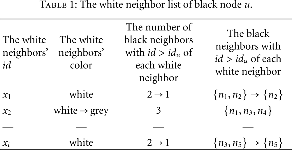
Each white node x with $k_{x} \geq 2$ sends packet ( $i d_{x}, C L_{x}, B_{x}$ ) to its neighbors, where $i d_{x}, C L_{x}$ and $B_{x}$ are the $i d$ , color and black neighbor set of x, respectively.

(2)

After black node u has received packets ( $i d_{x}, C L_{x}, B_{x}$ )s from its white neighbors, u saves the black nodes in $B_{x}$ of each packet into its 2-hop black neighbor set $N b_{1} (u)$ . And u constructs a 2 dimension table which saves its white neighbors’ $i d$ , color, the black neighbors with $i d > i d_{u}$ and the corresponding number of each white neighbor in each column.

(3)

For each black node u, we assume that there are at most t white neighbors. Note that $t \leq δ$ and $δ$ is the maximum node degree. Then u colors the white node $x_{i}$ grey which has the maximum value in the third column of current 2-dimension table, deletes all the common black neighbors between white nodes $x_{i}$ and $x_{j}$ ( $j \neq i$ and $1 \leq j \leq t$ ) and updates the numbers in the third column for remaining white nodes in the table.

(4)

For each black node u, repeat step (3) until all numbers in the third column of the table are zero.

As shown in Table 1, we assume that $x_{2}$ is the first node which would be colored grey for black node u. Then, u deletes the common nodes $n_{1}$ and $n_{3}$ in the fourth column and updates the number of black neighbors with $i d > i d_{u}$ of $x_{1}$ and $x_{t}$ , respectively. The updated details are presented behind symbol “→”.

Table 1

The white neighbor list of black node u.

The white neighbors’ $i d$	The white neighbors’ color	The number of black neighbors with $i d > i d_{u}$ of each white neighbor	The black neighbors with $i d > i d_{u}$ of each white neighbor
$x_{1}$	white	2→1	${n_{1}, n_{2}} \to {n_{2}}$
$x_{2}$	white→grey	3	${n_{1}, n_{3}, n_{4}}$
—	—	—	—
$x_{t}$	white	2→1	${n_{3}, n_{5}} \to {n_{5}}$

Procedure 2.

Coloring3(G, C, $V_{2 C}$ )

Input: A connected graph G, a black node set C and a grey node set $V_{2 C}$ .

Output: A node subset $V_{3 C}$ with coloring red.

(1)

Each grey node y and white node x send packet ( $i d_{y}, C L_{y}, B_{y}$ ) and ( $i d_{x}, C L_{x}, B_{x}$ ) to its neighbors respectively.

(2)

When a grey node $y_{j}$ which is a neighbor of y has received ( $i d_{y}, C L_{y}, B_{y}$ ), $y_{j}$ sends packet $C N = (i d_{y_{j}}, C L_{y_{j}}, i d_{y}, C L_{y}, B_{y})$ . When a grey node $y_{j}$ which is a neighbor of white node x has received ( $i d_{x}, C L_{x}, B_{x}$ ), $y_{j}$ sends $C N = (i d_{y_{j}}, C L_{y_{j}}, i d_{x}, C L_{x}, B_{x})$ . When a white node x has received ( $i d_{y}, C L_{y}, B_{y}$ ) from its grey neighbor y, x sends $C N = (i d_{x}, C L_{x}, i d_{y}, C L_{y}, B_{y})$ .

(3)

For each black node u in $B_{y}$ , let $N b_{2} (u)$ denote the 3-hop black neighbor set of u. Initially, $N b_{2} (u) = N b_{1} (u)$ . When u has received $(i d_{y_{j}}, C L_{y_{j}}, i d_{y}, C L_{y}, B_{y})$ or $(i d_{y_{j}}, C L_{y_{j}}, i d_{x}, C L_{x}, B_{x})$ from its grey neighbor $y_{j}$ , then $N b_{2} (u) = N b_{2} (u) ⋃ B_{y}$ or $N b_{2} (u) ⋃ B_{x}$ , respectively.

(4)

For each black node u in $B_{x}$ , when u has received ( $i d_{x}, C L_{x}, i d_{y}, C L_{y}, B_{y}$ ) from its white neighbor x, u saves the corresponding paths from u to $B_{y}$ into $P (u, B_{y})$ . For each black node w in $B_{y} ∖ N b_{2} (u)$ , u chooses a path $u x y w$ to connect with w. Then, color x red and let $N b_{2} (u) = N b_{2} (u) ⋃ B_{y}$ .

(5)

Each white node x sends ( $i d_{x}, C L_{x}, B_{x}$ ) again. When a white node $x_{i}$ has received ( $i d_{x}, C L_{x}, B_{x}$ ) from its neighbor x, $x_{i}$ sends ( $i d_{x_{i}}, C L_{x_{i}}, i d_{x}, C L_{x}, B_{x}$ ). For each black node u in $B_{x_{i}}$ , when u has received ( $i d_{x_{i}}, C L_{x_{i}}, i d_{x}, C L_{x}, B_{x}$ ), it saves the corresponding paths from u to $B_{x}$ into $P (u, B_{x})$ which saves all vertices in the paths. For each black node w in $B_{x} ∖ N b_{2} (u)$ with $i d_{w} > i d_{u}$ , a path $u x_{i} x w$ is chosen to connect u with w. Then, color $x_{i}$ and x red and let $N b_{2} (u) = N b_{2} (u) ⋃ B_{x}$ .

Lemma 5.

The message complexity of Algorithm 1 is $O (n^{2})$ and the time complexity is $O ({n δ}^{2})$ .

Proof.

By Procedures 1, and 2 and step (3) of Algorithm 1, each node needs to send constant messages to construct $V_{2 C}$ and $V_{3 C}$ , respectively. The message complexity of step (1) in Algorithm 1 is $O (n^{2})$ [17]. Hence, the message complexity of Algorithm 1 is $O (n^{2}) + O (n) + O (n) = O (n^{2})$ . In step (3) of Algorithm 1, note that x has at most 5 black neighbors [21]. Therefore, x needs $O (δ)$ time to compute its black neighbors’ information. And node u needs time $O (δ^{2})$ to compute ${N b}_{1} (u)$ in step (2) of Procedure 1. In the step (3) of Procedure 1, the number of rows of a 2-dimension table for node u is at most δ and the value in the fourth column of each row is no more than 5. Thus, each node u needs time $O (δ^{2})$ to choose white nodes such that u connects with ${N b}_{1} (u)$ at the end of step (4). Therefore, the time complexity of Procedure 1 is $n \cdot O (δ^{2} + δ^{2}) = O (n δ^{2})$ . In steps $(3, 4, and 5)$ of Procedure 2, node u needs time $O (δ^{2})$ for “union” operation to compute ${N b}_{2} (u)$ . Hence, the time complexity of Procedure 2 is $n \cdot O (δ^{2} + δ^{2} + δ^{2}) = O (n δ^{2})$ . In summary, the time complexity of Algorithm 1 is $n \cdot O (δ) + O (n δ^{2} + n δ^{2}) = O (n δ^{2})$ .

After Algorithm 1, we have accomplished a preliminary backbone. Then for each sensor node, it saves the angle information of its neighbors by measuring the direction of wireless signals [22].

Definition 6.

Given two vertices $u$ and $v$ , let $a (u, v)$ denote the angle of v relative to u.

For each vertex u in G, let $N (u)$ denote the neighbor set of u within 1-hop. Then, let $A (u) = {a (u, v) ∣ v \in N (u)}$ refer to the relative angle set of u. Furthermore, by measuring the strength of wireless signals [23], we can obtain the Euclidean length between u and v, which denotes as $d (u, v)$ . Hence, we have the following property.

Lemma 7.

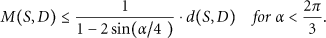
Given the destination D and two adjacent vertices u and v, if there exist $d (v, D)$ and $a (v, D)$ of v, then $d (u, D)$ and $a (u, D)$ of u can be computed.

Proof.

First, as shown in Figure 1, let u and v choose the same direction as the reference direction. It is trivial to show that $∠ u v D = π - a (v, D) + a (u, v) or π + a (v, D) - a (u, v)$ .

Then, based on the law of cosine, we have $\cos ∠ u v D = - \cos (a (v, D) - a (u, v))$ .

Then,

\begin{array}{l} d (u, D) \\ = \sqrt{d {(v, D)}^{2} + d {(u, v)}^{2} - 2 d (v, D) \cdot d (u, v) \cdot \cos ∠ u v D}, \end{array}

(1)

a (u, D) = {\begin{array}{l} a (u, v) - < u u D, & a (u, v) > a (a, D) \\ a (u, v) + < v u D, & a (u, v) \leq a (a, D) . \end{array}

(2)

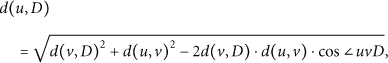
Therefore, we can obtain $d (u, D)$ and $a (u, D)$ for u.

Figure 1

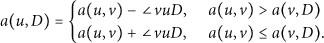
Compute $d (u, D)$ and $a (u, D)$ .

By Lemma 7, for each vertex u in graph G, u computes the angle set $A (u)$ and unites it into the preliminary infrastructure which has been built by Algorithm 1. Eventually, we have accomplished a path planning infrastructure. In the following, we propose a path planning algorithm with constant distance cost based on the infrastructure.

4. A Path Planning Algorithm

In [13], Lee et al. proposed the overhead of navigation algorithm. Let S denote the initial position and D be the destination. $M (S, D)$ denotes the length of moving path and $d (S, D)$ denotes the Euclidean length from S to D. Hence, we introduce a general definition.

Definition 8.

Given a constant $λ > 0$ , for any two positions S and D, if a path planning algorithm makes $M (S, D) \leq λ \cdot d (S, D)$ , then the algorithm guarantees a constant distance cost.

Before proposing our path planning algorithm, the destination data needs to be sent to sensor nodes by the infrastructure.

4.1. Send Destination Data

After the whole area has been monitored by a WSN, some sensor nodes would detect critical events when they have happened in the environment. Supposing that sensor node v has detected the event, then v will confirm the event point D by special measuring modules and transmit the packet $({i d}_{v}, d (v, D), a (v, D))$ based on the planning infrastructure. Later, when a sensor node u which is a neighbor of v has received the packet, u could compute $d (u, D)$ and $a (u, D)$ by Lemma 7. Therefore, the whole sensor nodes can gain destination information by communicating with its neighbors.

4.2. A Path Planning Algorithm in WSNs

After sensor nodes in the network have obtained information of destination D, the mobile node which denotes as M with enough energy will move to D automatically using the information stored in sensor nodes. Here, we assume that the communication and sensing range of M are the same with those of sensor node which are $R_{C}$ and $r_{s}$ , respectively. Then, we could release M in any position of the environment. For the simplicity of discussion, let M have the same location of a sensor node u in the network. That is, M seems to be u and can obtain $a (M, D)$ which is a duplicate of $a (u, D)$ . Therefore, without using localization, M can track its neighbors in the network to arrive at D. In the following, we describe the tracking process in detail.

Note that $N (M) = {v ∣ d (M, v) \leq R_{C}}$ denotes the neighbors of M and $A (M) = {a (M, v) ∣ v \in N (M)}$ refers to the relative angle set. Define $θ = ∠ v M D$ as the include angle of $a (M, v)$ and $a (M, D)$ for each v in $N (M)$ . Then, let M choose a neighbor u to make $θ = ∠ u M D$ minimum as its temporary target within range $R_{C}$ . It is trivial to show that if θ approximates zero, then $a (M, u)$ is the same as $a (M, D)$ which is the optimal direction of movement. In order to restrict the deviation of $a (M, D)$ and $a (M, u)$ by an upper bound, Algorithm 2 claims that the temporary optimal target u should be chosen in the sector $a (M, D) \pm α / 2 (α < 2 π / 3)$ within range $R_{C}$ . For a randomly deployed WSN with a high density of sensor nodes, we prove that there is at least one sensor node in the chosen sector with high probability which will guarantee a constant distance cost.

Algorithm 2: A path planning algorithm for mobile node (MSNA).

//Next(M) saves the temporary targets for M to track.

Input: A mobile node M, an initial position S and a destination D.

Output: A path consists of sensor nodes from S to D.

(1) Place mobile node M at the position S.

(2) Next(M) = NULL

(3) while M has not arrived at destination D

(4) do M updates a(M,D) and chooses an optimal temporary target in $a (M, D) \pm α / 2 (α < 2 π / 3)$ within range

$R_{C}$ from N(M)∖Next(M)

(5) if there is no condidate then

(6) M computes a virtual sensor node u′

(7) Call Algorithm 1 to update the planning infrastructure

(8) Call Procedure 3 to find a substituted path to bypass u′

(9) end if

(10) Add w into Next(M) and let M move to w

(11) end while

For an extreme situation where there is no sensor node in $a (M, D) \pm α / 2 (α < 2 π / 3)$ within range $R_{C}$ , Algorithm 2 designs a substituted moving path by computing virtual positions in the environment. Note that the network has been modeled as a UDG. If M finds that there is no node for current selection, then M computes a virtual sensor node $u^{'}$ on the direction $a (M, D)$ with $d (M, u^{'}) = 1$ . By Lemma 4, update Algorithm 1 to make the new path planning infrastructure regard virtual $u^{'}$ as a dominate by setting all the sensor nodes which monitor the position of $u^{'}$ be dominators in the network as dense as possible. Compared with M, $u^{'}$ is much closer to D. For simplicity, we assume there exists at least one candidate sensor node w in the sector $a (M, D) \pm α / 2 (α < 2 π / 3)$ within range $R_{C}$ for $u^{'}$ . Then, M can find a feasible solution from M to w in the new infrastructure using shortest vertex path algorithm [18]. Obviously, M cannot communicate with w for $d (M, w) > 1$ . Eventually, the algorithm also satisfies a constant distance cost which will be proven in the following.

The detailed algorithm is shown in Algorithm 2.

Procedure 3.

Finding a substituted path

Input: Next(M), M and $u'$ .

Output: A temporary target w and a feasible vertex path from M to w.

(1)

Compute $a (u', D)$ and choose an optimal temporary target in $a (u', D) \pm α / 2 (α < 2 π / 3)$ within range $R_{C}$ from $N (u') ∖ N e x t (M)$ .

(2)

Find a shortest vertex path $P (M, w)$ in the path planning infrastructure by the algorithm in [18].

To evaluate the performance of Algorithm 2, we assume that sensor nodes have been randomly deployed in a unit square. Then, we give the probability of nodes in each grid of a partition of this square using Chernoff's bound.

Lemma 9.

Given a randomly deployed node set V and a partition of unit square ${[0,1]}^{2}$ into grids with side length l, where $\sqrt{\log n / (c \cdot n)} \leq l < 1$ , then there exist constant c and $δ \in (0,1)$ , such that each grid contains at least $δ \cdot \log n / c$ nodes with high probability, where $n = | V |$ .

Proof.

Partition ${[0,1]}^{2}$ into $c n / \log n$ grids of equal size where $c < 1$ . Given a fixed small grid $Q_{j}$ , where $1 \leq j \leq c n / \log n$ , if node i falls into grid $Q_{j}$ , then $X_{i} = 1$ , otherwise $X_{i} = 0$ . Here $X_{i}$ is a random variable. According to the observation, all random variables $X_{i}$ s, where $1 \leq i \leq n$ , are independent and the probability $P (X_{i} = 1) = \log n / c n$ . Let $= \sum_{i = 1}^{n} X_{i}$ , then

\begin{matrix} E (X) = E (\sum_{i = 1}^{n} X_{i}) = \sum_{i = 1}^{n} E (X_{i}) = \frac{n \cdot \log n}{c n} = \frac{\log n}{c} . \end{matrix}

(3)

Applying the Chernoff's bound, we have

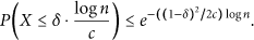
\begin{matrix} P (X \leq δ \cdot \frac{\log n}{c}) \leq e^{- ((1 - δ)^{2} / 2 c) \log n} . \end{matrix}

(4)

So, for all grids in unit square, we denote the number of nodes in $Q_{j^{'}} (Q_{j^{'}} \in {Q_{j}})$ as $X^{'}$ , and the probability of $X^{'} < δ \cdot \log n / c$ is $P (δ)$ , then we get

\begin{array}{l} P (δ) & \leq & \frac{c n}{log n} \cdot e^{- ({(1 - δ)}^{2} / 2 c) log n} \\ = & e^{- ({(1 - δ)}^{2} / 2 c) log n + ln (c n / log n)} \\ < & e^{- ({(1 - δ)}^{2} / 2 c) log n + log (c n / log n)} . \end{array}

(5)

Using $c = 0.2$ and $δ = 0.1$ , we obtain

\begin{array}{l} P (0.1) \leq \frac{c n}{\log n} \cdot e^{- ((1 - δ)^{2} / 2 c) \log n} \\ < e^{- ((1 - δ)^{2} / 2 c) \log n + \log (c n / \log n)} \\ < e^{- 2 \log n + \log n + \log c - loglog n} < \frac{1}{n} . \end{array}

(6)

Then, based on Lemma 9, we introduce the probability of sensor nodes existing in the sector $a (M, D) \pm α / 2 (α < 2 π / 3)$ within range $R_{C}$ .

Theorem 10.

Given a random node set V and the communicating range $R_{C}$ of sensor node, if $n \cdot R_{C}^{2} > 8 \cdot \log n$ , then there exist constant c and $δ \in (0,1)$ , such that each sector with angle α of the mobile node has $δ \cdot \log n / c$ neighbors with high probability, where $n = | V |$ .

Proof.

By Lemma 9, when the mobile node M is in a grid $Q_{j}$ , adjust the communication range such that $R_{C} = 2 \sqrt{2} \cdot l > 2 \sqrt{2} \cdot \sqrt{\log n / n}$ . Then, we get that the mobile node that can communicate with at least 8 neighbors in its adjacent grids. While the mobile node separates the communicating disk into sectors with angle α, the area of each sector is $S_{C} = 4 α l^{2}$ . Note that if $0.25 < α < 2 π / 3$ , then $S_{C} > l^{2}$ . Denote the probability of each sector contains at least $δ \cdot \log n / c$ nodes as $P (δ)$ , and then we have

\begin{matrix} P (δ) \geq 1 - e^{- ((1 - δ)^{2} / 2 c) \log n + \log (c n / \log n)} . \end{matrix}

(7)

By setting $c = 0.2$ , $δ = 0.1$ , and denoting the probability which has at least $\log n / 2$ neighbors in a sector as $P_{r}$ , we obtain $P_{r} \geq 1 - 1 / n$ .

In order to analyze the distance cost of path by Algorithm 2, we propose a lemma when there is no extreme case happening.

Lemma 11.

Let $v_{0} v_{1} \dots v_{k + 1}$ be the path of mobile node M in Algorithm 2 without any extreme case, where $v_{0} = S$ is the initial position and $v_{k + 1} = D$ is the destination. Then

\begin{matrix} M (S, D) \leq \frac{1}{1 - 2 \sin (α / 4)} \cdot d (S, D) for α < \frac{2 π}{3} . \end{matrix}

(8)

Proof.

Note that $d (u, v)$ is the Euclidean length from u to v and abbreviates to $u v$ . Based on the choosing rule in Algorithm 2, we know $v_{k - 1} v_{k} < v_{k - 1} v_{k + 1}$ . Set a dot $v_{k}^{'}$ on dotted line $v_{k - 1} v_{k + 1}$ satisfying $v_{k - 1} v_{k}^{'} = v_{k - 1} v_{k}$ , as shown in Figure 2. Then we have $v_{k} v_{k + 1} < v_{k} v_{k}^{'}$ $+ v_{k}^{'} v_{k + 1}$ by triangle inequality. Obviously, for any $v_{i}$ $(1 \leq i \leq k)$ , there is $θ_{i} = ∠ v_{i} M D \leq α / 2$ , where $α < 2 π / 3$ . Then, $v_{k} v_{k}^{'} = 2 \sin (∠ v_{k} v_{k - 1} v_{k}^{'}$ / $2) \cdot v_{k - 1} v_{k} \leq 2 \sin (α / 4) \cdot v_{k - 1} v_{k}$ . Because $v_{k}^{'} v_{k + 1} = v_{k - 1} v_{k + 1} - v_{k - 1} v_{k}^{'}$ , we have $v_{k - 1} v_{k} = v_{k - 1} v_{k}^{'} = v_{k - 1} v_{k + 1} - v_{k}^{'} v_{k + 1} \leq v_{k - 1} v_{k + 1} + v_{k} v_{k}^{'} - v_{k} v_{k + 1} \leq v_{k - 1} v_{k + 1} + 2 \sin (α / 4) \cdot v_{k - 1} v_{k} - v_{k} v_{k + 1}$ . Hence, $v_{k - 1} v_{k + 1} - v_{k} v_{k + 1} \geq (1 - 2 \sin (α / 4)) v_{k - 1} v_{k}$ .

Furthermore,

\begin{array}{l} M (S, D) & = & \sum_{i = 0}^{k} d (v_{i}, v_{i + 1}) \leq \frac{1}{1 - 2 sin (α / 4)} \\ \cdot \sum_{i = 0}^{k} (v_{i} v_{k + 1} - v_{i + 1} v_{k + 1}) \\ = & \frac{1}{1 - 2 sin (α / 4) v_{0} v_{k + 1}} . \end{array}

(9)

Figure 2

A vertex path from $v_{k - 1}$ to $v_{k + 1}$ .

Without loss of generality, we assume that there exists only one extreme case during planning a path in Algorithm 2.

Theorem 12.

Let $v_{0} v_{1} \dots v_{k + 1}$ be the path of mobile node M in Algorithm 2 with an extreme case, where $v_{0} = S$ is the initial position and $v_{k + 1} = D$ is the destination. Then

\begin{matrix} M (S, D) \leq \frac{10}{1 - 2 \sin (α / 4)} \cdot d (S, D) for α < 2 π / 3 . \end{matrix}

(10)

Proof.

We assume that the extreme case happens at $v_{j}$ . That is, $v_{j + 1}$ is chosen by call Procedure 3 with $d (v_{j}, v_{j + 1}) > 1$ . Let u denote the virtual node. Then, by the path planning infrastructure and Lemma 4, we have that the shortest vertex path $h^{'} (v_{j}, v_{j + 1})$ from $v_{j}$ to $v_{j + 1}$ satisfing $h^{'}$ ( $v_{j}, v_{j + 1}) \leq 5 (h (v_{j}, u) + h (u, v_{j + 1}))$ . Because for any two adjacent sensor nodes $u_{1}$ and $u_{2}$ in the network which has been modeled as a UDG, we obtain $d (u_{1}, u_{2}) \leq h (u_{1}, u_{2})$ . Hence, the length of moving path from $v_{j}$ to $v_{j + 1}$ which is denoted as $d^{'} (v_{j}, v_{j + 1})$ satisfies $d^{'} (v_{j}, v_{j + 1}) \leq h^{'} (v_{j}, v_{j + 1})$ . By the triangle inequality, there is $d (v_{j}, u) + d (u, v_{j + 1}) > d (v_{j}, v_{j + 1}) > 1$ . Then, $h (v_{j}, u) + h (u, v_{j + 1}) = 2 < 2 d (v_{j}, v_{j + 1})$ . Furthermore, $d^{'} (v_{j}, v_{j + 1}) \leq 10 d (v_{j}, v_{j + 1})$ . Therefore, by Lemma 11,

\begin{matrix} M (S, D) \leq \frac{10}{1 - 2 \sin (α / 4)} \cdot d (S, D) . \end{matrix}

(11)

Note that each $v_{i}$ is a realistic sensor node. The virtual node is used for updating the path planning infrastructure for an extreme situation under a very low probability. If there are several extreme cases, the proof of Theorem 12 could be extended easily with the same constant ratio.

5. Simulation Results

As mentioned previously, many studies have shown novel algorithms for the infrastructures. In this section, firstly we use VC++6.0 to conduct simulations to compare the performance of algorithm IRC with those of GOC and ICDS in [19, 20], respectively. The area of simulation is a virtual square $S_{1}$ of $100 \times 100$ , and nodes are randomly distributed in $S_{1}$ . The number of nodes denoted by N is increased by 10 from 10 to 100 and the maximum transmission range $R_{C}$ is assigned 20, 25, 30, and 35. For distinct nodes u and v, if and only if the Euclidean distance $d (u, v) \leq R_{C}$ , u and v could communicate with each other. For the same settings under different transmission ranges, we randomly create 100 connected graphs for each N and accordingly construct the infrastructure for each connected graph. And for each infrastructure, we compute its size and diameter.

Figure 3 shows the infrastructure sizes of algorithm IRC, GOC, and ICDS under the different $R_{C}$ s. In this figure, since more nodes are needed in a bigger network for guaranteed overhead, all the sizes of infrastructures produced by algorithm IRC, GOC, and ICDS increase when the number of nodes increases. For the network with a small amount of nodes, these infrastructure sizes are almost equal. While nodes increase, algorithm IRC presents a better performance for different $R_{C}$ s.

Figure 3

Infrastructure sizes.

Figure 4 shows the diameters of graph G and infrastructures produced by algorithm IRC and GOC. When $R_{C}$ is small, the difference of diameters between two infrastructures and graph G is small. But as $R_{C}$ increases, the difference goes larger what keeps pace with that of the infrastructure size in Figure 3. However, for different $R_{C}$ s, the difference of diameter between algorithm IRC and GOC is very small which implicits that there may exist several redundant nodes in the infrastructure which produced by GOC.

Figure 4

Diameters.

Then, based on the infrastructure which has been constructed, we use VC++6.0 and Matlab 7.0 to evaluate algorithm MSNA. To compare with the distance cost of algorithm ANHC in [13], we set the environment and network parameters to be the same with those in [13]. Table 2 shows the detailed parameters which will be used. We provide four different ways for sensor nodes deployment: (1) 99 nodes are deployed in $S_{2}$ uniformly, the interval of each node is 100 m; (2) 114 nodes are deployed in $S_{2}$ with a hole in the center; (3) 100 nodes are randomly deployed in $S_{2}$ ; (4) 150 nodes are randomly deployed in $S_{2}$ .

Table 2

Simulation parameters.

Parameters	Value
The monitoring area $S_{2}$	1100 × 900 m²
Communication range $R_{C}$	150 m
Sensing range $r_{s}$	15 m
The number of deployed sensor nodes	99, 114, 100, 150
Identifiers	$1 - N$

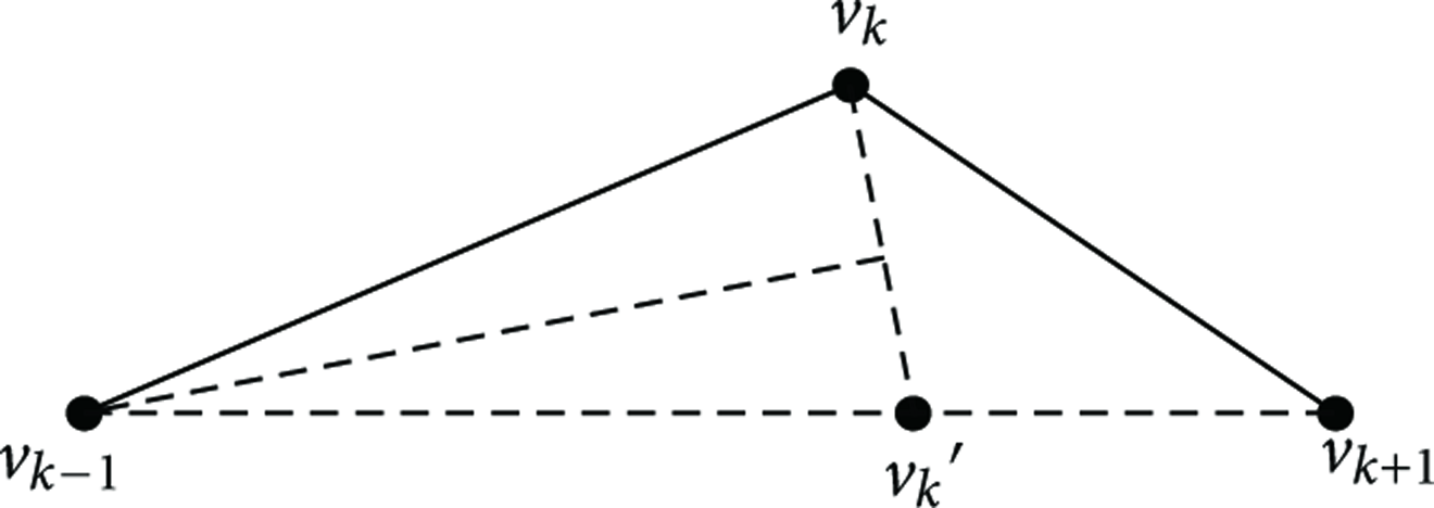
In Figure 5, four different planning paths are presented under corresponding deployed ways. By tracking the realistic sensor nodes in the network, all the paths can be defined as directed vertex paths in the graph which is modeled by a WSN. In each figure, we use the symbol “*” and “☆” to stand for the initial position and destination of a planning path, respectively. The dots which are encircled by “△” are represented as the sensor nodes tracked by mobile node. A dashed circle denotes the transmitting range of wireless signal. In Figure 5(a), at the beginning, the mobile node chooses the optimal sensor nodes from its neighbors as the temporary target. Without using a localization technique, the mobile node tracks the temporary targets which could be computed by algorithm MSNA in the uniform network. In Figure 5(b), for the given initial position, although there is a hole in the center of $S_{2}$ , the mobile node has not encountered any extreme cases during selecting temporary target. So, the path consists of a node set alongside the border of hole. In Figure 5(c), an extreme case has happened in algorithm MSNA. The two square symbols “□” show the virtual nodes which were computed in algorithm MSNA with being closer to the destination in the path planning infrastructure. In Figure 5(d), the network is quite dense such that there is no extreme case for the mobile node. For the locations of sensor nodes in the path, we find that they almost distributed along the straight line from start to destination.

Figure 5

Trajectories of the mobile node by MSNA.

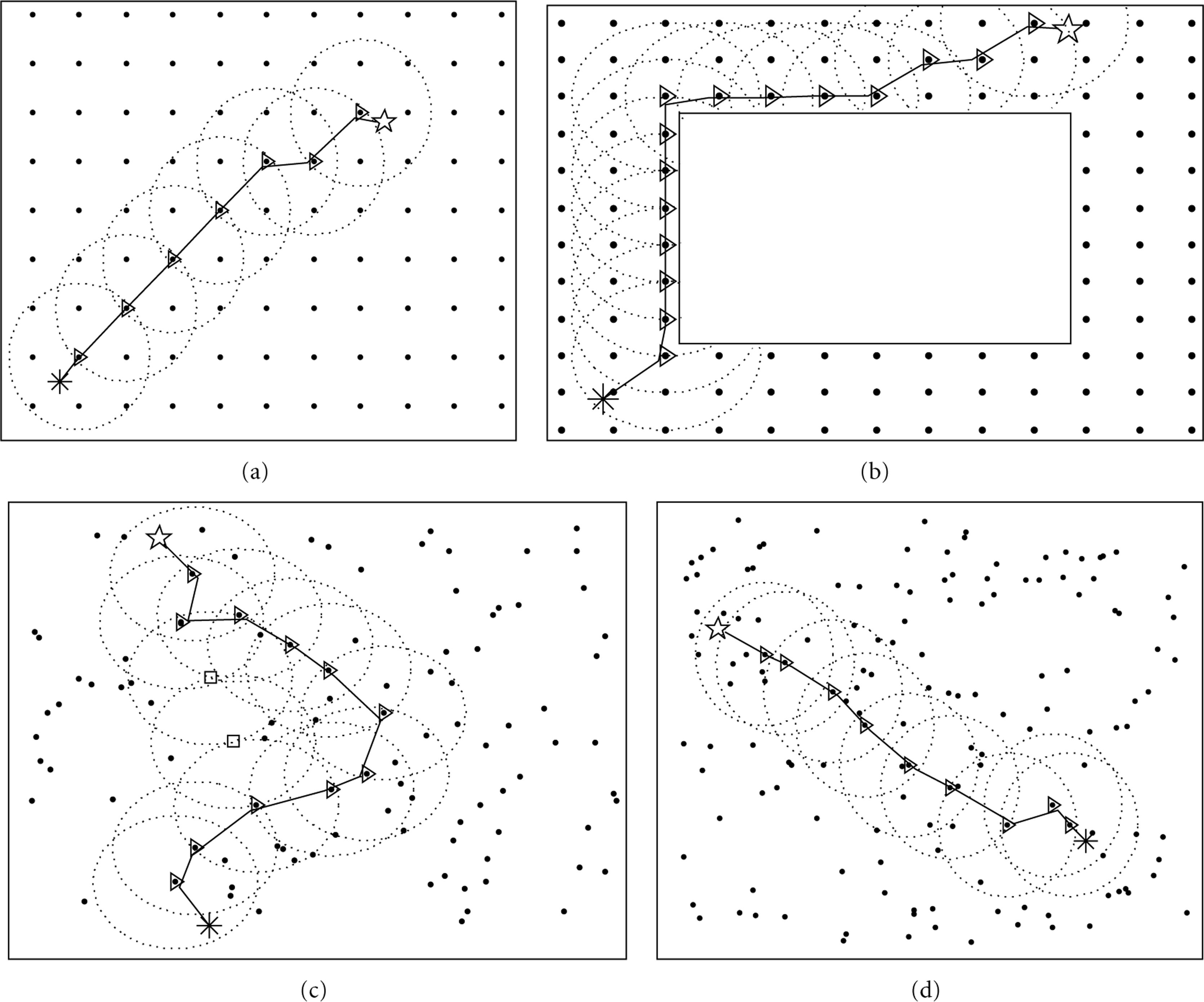
In [13], the algorithm ANHC using average hop-count of neighbors is the first one concerning the cost of a navigating path without localization. In the initial phase, each sensor node sets up its hop count value to the destination. Then, every sensor node computes the value anhc by communicating with its neighbors. It implicated that sensor nodes which are closer to the destination would have smaller anhc compared with the ones which are far away from the destination. The mobile node computes its anhc at its present location. By judging the variation of value anhc, the mobile node revises its direction. The disadvantage of this algorithm is that although the decreasing of anhc shows that the mobile node is moving to the destination, it cannot indicate the deviation between current direction and the optimal direction which may lead to a high cost. In algorithm MSNA, at current position, the mobile node chooses the optimal temporary target which makes the deviation between direction of movement and the optimal direction be minimum. But there also exists the disadvantage in MSNA because we cannot guarantee there must have candidates in the sector $a (M, D) \pm α / 2$ ( $α < 2 π / 3$ ) within $R_{C}$ for mobile node M.

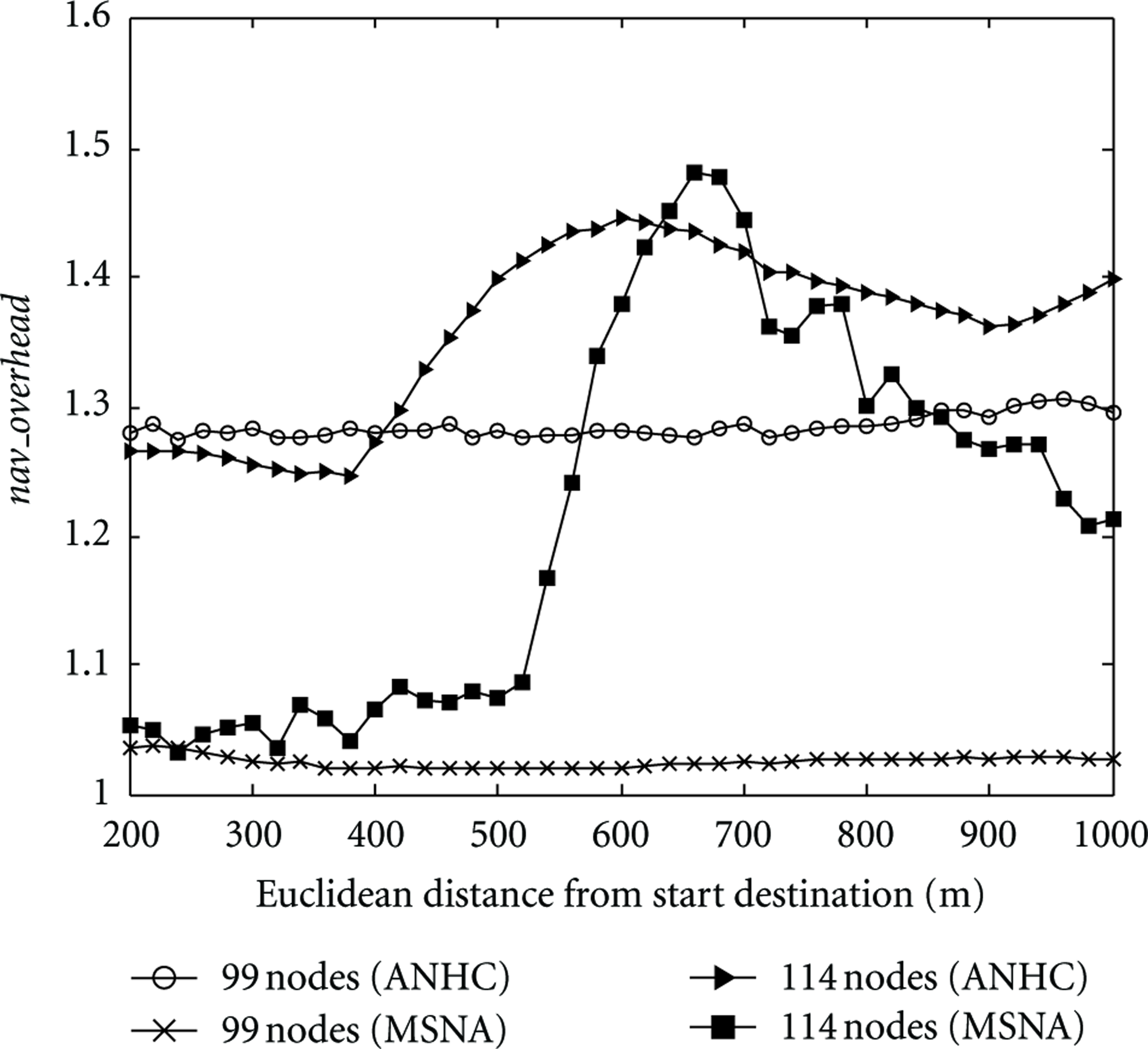
In the following, we randomly set the initial position $S$ and the destination D with 200 m $\leq d (S, D) \leq 1000$ m. Through employing a lot of randomly deployed networks, the average costs of paths have been presented in Figure 6 for the predefined shortest Euclidean distance. It shows that ${n a v_o v e r h e a d}_{ANHC} > {n a v_o v e r h e a d}_{MSNA}$ for the first deployed way. And under the second way, ${n a v_o v e r h e a d}_{ANHC} > {n a v_o v e r h e a d}_{MSNA}$ is almost true for different predefined situations.

Figure 6

The path cost for a uniform deployed network.

Figure 7 shows that the average costs of paths under four different deployed ways of the network. We randomly set the initial position Sand the destination D in the environment. Through a lot of simulations, we find that the cost of algorithm MSNA is smaller than the algorithm ANHC for each deployed way.

Figure 7

The average path cost for four different deployed ways.

6. Conclusion

In this paper, by characterizing the navigation problem as a path planning problem, we first present a distributed algorithm to construct a path planning infrastructure by uniting the neighbors’ information of each sensor node into a CDS. Then, we propose a path planning algorithm to generate an effective path in the network even under an extreme case. We prove that the distributed algorithm has low time and message complexity and the path planning algorithm guarantees a constant distance cost. Simulation results show that the algorithms produce a smaller infrastructure size and a distance cost. Due to frequent node and link failure, which are inherent in WSNs, to construct a robust a path planning algorithm is our further work.

Footnotes

Acknowledgment

This work is supported by the National Natural Science Foundation of China under Grants no. 61070169, 61170021 and 61201212, The Natural Science Foundation of Jiangsu Province under Grant no. BK2011376, The Specialized Research Foundation for the Doctoral Program of Higher Education of China no. 20103201110018, The Application Foundation Research of Suzhou of China No. SYG201118, SYG201240, SYG201239 and sponsored by the Qing Lan Project.

References

Al-Turjman

F. M.

Hassanein

H. S.

Ibnkahla

M. A.

Connectivity optimization for wireless sensor networks applied to forest monitoring

Proceedings of the IEEE International Conference on Communications (ICC '09)

June 2009

1 6

2-s2.0-70449505570

10.1109/ICC.2009.5198845

Postolache

O. A.

Dias Pereira

J. M.

Silva Girão

P. M. B.

Smart sensors network for air quality monitoring applications

IEEE Transactions on Instrumentation and Measurement 2009 58 9 3253 3262

2-s2.0-69249220119

10.1109/TIM.2009.2022372

Chen

C. W.

Wang

Chain-type wireless sensor network for monitoring long range infrastructures: architecture and protocols

International Journal of Distributed Sensor Networks 2008 4 4 287 314

2-s2.0-54249162967

10.1080/15501320701260261

Casey

Lim

Dozier

A sensor network architecture for Tsunami detection and response

International Journal of Distributed Sensor Networks 2008 4 1 28 43

2-s2.0-38749106968

10.1080/15501320701774675

Borenstein

Everett

H. R.

Navigating Mobile Robots: Sensors and Techniques 1992

New York, NY, USA

John Wiley & Sons

Sinha

Sivakumar

Bharghavan

Enhancing ad hoc routing with dynamic virtual infrastructures

Proceedings of the 20th Annual Joint Conference of the IEEE Computer and Communications Societies (INFOCOM '01)

April 2001

1763 1772

2-s2.0-0035017882

Fonseca

Gnawali

Jamieson

Moss

Levis

Collection tree protocol

Proceedings of the 7th ACM Conference on Embedded Networked Sensor Systems (SenSys '09)

November 2009

usa

1 14

2-s2.0-74549185267

10.1145/1644038.1644040

Moon

T. K.

Kuc

T. Y.

An integrated intelligent control architecture for mobile robot navigation within sensor network environment

Proceedings of the IEEE/RSJ International Conference on Intelligent Robots and Systems (IROS '04)

October 2004

565 570

2-s2.0-14044253571

Briggs

A. J.

Detweiler

Scharstein

Vandenberg-Rodes

Expected shortest paths for landmark-based robot navigation

International Journal of Robotics Research 2004 23 7-8 717 728

2-s2.0-3142768944

10.1177/0278364904045467

10.

De Rosa

Rus

Distributed Algorithms for Guiding Navigation across a Sensor Network

Proceedings of the 9th Annual International Conference on Mobile Computing and Networking (MobiCom '03)

September 2003

313 325

2-s2.0-1542378235

11.

Jiang

Zhang

Novel navigation algorithm for wireless sensor networks without information of locations

Proceedings of the Global Communications Conference (GLOBECOM '11)

2011

1 6

12.

Zhan

Yang

Chen

Efficient emergency rescue navigation with wireless sensor networks

Journal of Information Science and Engineering 2011 27 1 51 64

2-s2.0-79751517489

13.

Lee

W. Y.

Hur

Eom

D. S.

Navigation of mobile node in wireless sensor networks without localization

Proceedings of the IEEE International Conference on Multisensor Fusion and Integration for Intelligent Systems (MFI '08)

August 2008

1 7

2-s2.0-67650512290

10.1109/MFI.2008.4648099

14.

Liu

Wang

Yang

Sensor network navigation without locations

Proceedings of the 28th IEEE Conference on Computer Communications (INFOCOM '09)

April 2009

2419 2427

2-s2.0-70349686611

10.1109/INFCOM.2009.5062169

15.

Tseng

Y. C.

Pan

M. S.

Tsai

Y. Y.

Wireless sensor networks for emergency navigation

Computer 2006 39 7 55 62

2-s2.0-33746369139

10.1109/MC.2006.248

16.

Wei

Information potential fields navigation in wireless Ad-Hoc sensor networks

Sensors 2011 11 5 4794 4807

2-s2.0-79957785921

10.3390/s110504794

17.

Stojmenovic

Seddigh

Zunic

Dominating sets and neighbor elimination-based broadcasting algorithms in wireless networks

IEEE Transactions on Parallel and Distributed Systems 2002 13 1 14 25

2-s2.0-0036377260

10.1109/71.980024

18.

Suurballe

J. W.

Tarjan

R. E.

A quick method for finding shortest pairs of disjoint paths

Networks 1984 14 2 325 336

2-s2.0-0021441708

19.

Lee

Howard

Constant approximation for virtual backbone construction with Guaranteed Routing Cost in wireless sensor networks

Proceedings of the IEEE International Conference on Computer Communications (INFOCOM '11)

April 2011

1737 1744

2-s2.0-79960877514

10.1109/INFCOM.2011.5934967

20.

Wang

X. Y.

Geometric spanners for wireless ad hoc networks

Proceedings of the 22nd IEEE International Conference on Distributed Systems (ICDCS '02)

July 2002

171 178

2-s2.0-0036373267

21.

Wan

P. J.

Alzoubi

K. M.

Frieder

Distributed construction of connected dominating set in wireless ad hoc networks

Mobile Networks and Applications 2004 9 2 141 149

2-s2.0-1642408650

10.1023/B:MONE.0000013625.87793.13

22.

Niculescu

Nath

Ad hoc positioning system (APS) using AOA

Proceedings of the 22nd Annual Joint Conference on the IEEE Computer and Communications Societies (INFOCOM '03)

April 2003

1734 1743

2-s2.0-0041973656

23.

Girod

Bychkovskiy

Elson

Estrin

Locating tiny sensors in time and space: a case study

Proceedings of the International Conference on Computer Design (ICCD '02) VLSI in Copmuters and Processors

September 2002

214 219

2-s2.0-0036396923

A Path Planning Algorithm with a Guaranteed Distance Cost in Wireless Sensor Networks

Abstract

1. Introduction

2. Related Work

3. Network Model

Definition 1.

Definition 2.

Lemma 3 (see [19]).

Lemma 4.

Proof.

Algorithm 1: Constructing the preliminary planning infrastructure (IRC).

Procedure 1.

Procedure 2.

Lemma 5.

Proof.

Definition 6.

Lemma 7.

Proof.

4. A Path Planning Algorithm

Definition 8.

4.1. Send Destination Data

4.2. A Path Planning Algorithm in WSNs

Algorithm 2: A path planning algorithm for mobile node (MSNA).

Procedure 3.

Lemma 9.

Proof.

Theorem 10.

Proof.

Lemma 11.

Proof.

Theorem 12.

Proof.

5. Simulation Results

6. Conclusion

Footnotes

Acknowledgment

References