Rendezvous Data Collection Using a Mobile Element in Heterogeneous Sensor Networks

Abstract

We study the rendezvous data collection problem for the Mobile Element (ME) in heterogeneous sensor networks where data generation rates of sensors are distinct. The link quality is instable in our network model and the sensory data cannot be aggregated when transmitting. The Mobile Element is able to efficiently collect network wide data within a given delay bound; meanwhile the network eliminates the energy bottleneck to prolong its lifetime. For case study, we consider the trajectory planning for both Mobile Relay and Mobile Sink on a tree-shaped network. In the Mobile Relay case where the ME's trajectory must pass through a sink to upload sensory data for further processing, an O(n lg n) algorithm named RP-MR is proposed to approach (1) the optimal Rendezvous Points (RPs) to collect global sensory data; (2) the optimal data collection trajectory for the Mobile Relay to gather the cached data from RPs. In the Mobile Sink case where the Mobile Element can process the sensory on its motion, we develop an O(n lg²n) algorithm named RP-MS to recursively investigate the optimal solution. Both the theoretical analysis and extensive simulations verify the correctness and effectiveness of proposals.

1. Introduction

Since the emergence, Wireless Sensor Networks (WSNs) undertake intensive data collection during the sensing period. However, the limited energy storage of tiny sensors involved in a WSN harshly confines their ability of transmitting the acquired data. As a result, the premature death of several sensors always perturbs the connectivity of the network. To address this issue, some researchers [1–3] introduced a novel data gathering technique that combines controlled mobility and rendezvous-based data collection, where sensors first forward their sensing data to several Rendezvous Points (RPs), and then, tell a Mobile Element (ME) to pick up the cached data for further processing. A critical issue in such method is conserving limited energy and maximizing network lifetime.

To date, there is a broad range of literatures on improving the utility of this mobility-based strategy, managing to reduce the total data transmission load taken by the whole WSN. Although many of these prior efforts were able to present some optimal or near optimal solutions, most of these works based on several impractical assumptions. That is, the link quality is assumed fair enough; the data generation rates of sensors (In this paper, the words sensor and sensor node are used interchangeably.) are identical, and data can be fused when transmitting.

Generally, such assumptions cannot offer a holistic view of typical properties in WSNs for three reasons. First of all, medium quality and paths self-interfere can trigger packets loss and retransmission that consequently affect the link quality. As a result, the wireless link cannot stay in a stable condition, and data packet cannot be successfully delivered to the destination in each transmission. Secondly, collecting data like images from distant area of battlefield cannot be fused when transmitting. Therefore, the energy consumption of data transmission cannot be calculated as in previous works [1–3]. Thirdly, data generation rates on distinct sensors are usually diverse depending on the varying monitoring objectives in the network. For example, in monitoring environmental habitat, some sensors maybe indicated to observe the vibration frequency of the ground, while others are allocated to probe the local humidity. Apparently, the rates on these devices are not the same.

Basically, such properties which we term heterogeneous feature among sensor nodes mirror dynamic properties of WSNs, therefore requires rational handling. The significance of heterogeneous feature among sensor nodes lies in that, it captures the uncertain property of WSNs, which assists us to conduct in-depth analysis on mobility-based techniques, that is, locating RP in the “hot space” where data generation rate is high. As the basic assumptions in previous efforts are revealed to be impractical, the introduction of heterogeneous feature will trigger a big change in the optimization structure like maximizing network lifetime or minimizing the cost of communication, and so, many previous algorithms, which assumed sensor have the same data generation rate, cannot be mapped into this typical scenario.

In this paper, we are focusing on rendezvous planning in WSNs by taking the heterogeneous feature into consideration. In our network model, we adopt ETX [4] metric to measure the link quality considering the lossy link and the interference from hidden terminal. The data type and generation rate here are disparate from sensor to sensor; therefore the data cannot be fused when transmitting. Our goal is to find a ME moving trajectory and corresponding RPs, so as to minimize total energy consumption on in-network data communication. (In-network data communication represents the total data transmission cost for gathering global sensory data.) We formulate such an optimization problem as Minimum-Energy Rendezvous Point Selection Problem (shown in Figure 1). For case study, we consider two cases where the Mobile Element is Mobile Relay and Mobile Sink (Mobile Sink is also called Mobile Base Station in some literatures.), respectively. In the Mobile Relay case, the sensing data are first forwarded to several RPs for caching. Then, a Mobile Relay reaches each RP to download the cached data and then upload them at the Sink's site. In the Mobile Sink case, the Mobile Sink does data processing while it downloads the sensing data from each RP, with no need for uploading data at fixed point.

Figure 1

An example of Rendezvous Point Selection Problem. The circle represents sensor nodes and the square stands for Rendezvous Point. Notice that the darkness of circles varies with data generation rate.

Our contribution can be summarized as follows.

• (1)

We investigate the heterogeneous feature of sensors in WSNs and formulate rendezvous planning problems based on practical assumptions. In our network model, the link quality is measured by ETX; the data generation rates are disparate and cannot be fused when transmitting.

(2)

For case study, we consider two cases where the ME is Mobile Relay and Mobile Sink, respectively. In the Mobile Relay case, we propose an $O(n\hspace{0.17em}\text{lg}\hspace{0.17em}n)$ algorithm named RP-MR to achieve the optimal solution in tree-shaped topology. In the Mobile Sink case, we propose an $O(n\hspace{0.17em}\text{l}{\text{g}}^2\hspace{0.17em}n)$ algorithm to achieve the optimal solution under the same settings.

(3)

To the best of our knowledge, our work is the first attempt to consider heterogeneous feature of sensor nodes, which will trigger different data generation rate, and undermine the mechanism, aggregation. Ignoring such considerations will possibly lead to a higher energy burden on in-network data transmission.

The rest of paper is organized as follows. Section 2 reviews relevant work about rendezvous planning. Section 3 gives a brief description of our problems. Section 4 and Section 5 investigate the rendezvous planning problem in two cases, Mobile Relay and Mobile Sink, respectively. We evaluate the performance of our proposed algorithms in Section 6 and conclude our paper in Section 7.

2. Related Work

Typically, the Mobile Element is either Mobile Relay or Mobile Sink. The mobility of the ME is uncontrollable or controllable.

The basic idea of the uncontrollable case has been proposed by Shah et al. in their work Data Mules [5, 6]. The mobile relays, called MULEs, are used to collecting data from the sensors via single-hop transmission. Kim et al. [7] proposes protocol, SEAD, to find a tradeoff between the packet transmission delay and the energy consumption of reconfiguring the tree topology. The mobile sinks randomly access the tree from specified sensors (Access Point). As mobile sinks move freely, the communication between mobile sinks and Access Point can be multihop. Luo et al. [8] investigate the approach that makes use of a mobile sink for balancing the traffic load and in turn improving network lifetime. They engineer a routing protocol, MobiRoute, to effectively support sink mobility. Tian et al. [9] design protocol, AVRP, to adopt Voronoi scoping plus dynamic anchor selection to handle free and unpredictable moving of mobile sink, and protocol, TRAIL, to use the trail of mobile sink for guiding packet forwarding. The use of mobile elements with predictable pattern has been addressed in [10–16]. As the movements of the mobile elements in these works are fully controllable, the trajectories can be planed and routing protocol can be designed using the prediction.

The sensors first send their data to rendezvous point [1, 2], then the mobile sink visits these RPs to collect data via single-hop transmission. As the multihop routing between the sensors to the stationary sink is reduced to a smaller number of hops, the energy therefore gets reserved. Our previous work [17] falls into this category, which only considers the Mobile Relay case. To additively update the routing structure of data collection for mobile sink, Li et al. [18] propose protocol to only perform a local modification to update the routing structure, while the routing performance is bounded and controlled compared to the optimal performance.

3. Basic Assumptions and Network Model

In this section, we give our basic assumptions and present the network model.

3.1. Basic Assumptions

• (1)

  We assume that wireless communication is the dominating energy-consuming factor and hence omit other energy consuming functions such as sensing and processing.

• (2)

  We assume that the ME roams in the network to collect all those sensory data by visiting a series of RPs, with a required data collection delay bound D. The delay bound can be measured by the maximum distance L that the mobile sink is allowed to move. The location of sensor nodes can be calculated by localization algorithm [19].

• (3)

  We assume that each transmission (regardless of success or failure) costs equivalent energy. Thus, the energy consumption for delivering a data packet from a node to its neighbor is proportional to the transmission count until the neighbor receives the packet successfully.

• (4)

  We assume that the storage capacity of sensors is large enough to buffer the sensing data during a collection period. Several recent sensor network platforms [20] are equipped with 32 512MB MAC or NAND flash with ultralow power consumption.

• (5)

  We assume that data cannot be fused at any intermediate node before it arrives at the ME. Data gathering without aggregation has been applied in many scenarios like battlefield surveillance, habitat monitoring, which is dominated by the heterogeneous data.

3.2. Network Model

We consider a WSN with a set of ℵ nodes, where $|\aleph |=n$ . A link $l(i,j)\in Ł$ exists if and only if the Euclidean distance between the sensor nodes is shorter than the transmission range R. Let $r(i)$ be the data generation rate (packet/min) at node i, and $c_l(i,j)$ represents the ETX of link $l(i,j)\in Ł$ .

Initially, we assume each sensor has equivalent energy E, and each sensor cost identical energy e to transmit a data packet in each link. Thus, the energy consumption for transmitting one data packet from node i to its neighbor node j is $e·c_l(i,j)$ . Denote ${\iota }^{\text{out}}(i)$ and ${\iota }^{\text{in}}(i)$ the sets of outgoing and incoming links at node i. On link l, denote $r_l(i)$ the data generated from node i that is attributed to link l. The network lifetime T here is defined as the time when the first node dies.

4. Problem Formulation

In this section, we first present the description and formal definition of our problem and then give the formulation and list the characteristics of the problem.

4.1. Problem Definition

In our problem, a plenty of sensors must deliver their cached data to a Mobile Element within time interval D. The data generation rate on distinct sensors is different. Our objective is to find a data collection trajectory for the ME, such trajectory consists of several RPs between which the ME moves and at which they download data. On the other hand, RPs cache the global data of the network and upload them to the ME via short-range transmission when it passes by. The energy consumption for global data transmission should be minimized under the constraint that the ME must cover its trajectory before it depletes energy or the time interval D. We name this problem as Minimum-Energy Rendezvous Point Selection Problem (MRPSP). The formal definition can be given as follows.

Definition 1 (Minimum-Energy Rendezvous Point Selection Problem).

Given a set of sensors ℵ and the maximum allowable trajectory length $L={\nu }_{\text{ME}}·D$ of ME, we are aiming to find (1) a set of RPs that cache the global data of the network, so as to minimize the in-network transmission cost and (2) a length-constrained data collection trajectory (Here the length-constrained data collection trajectory stands for the trajectory whose length is shorter than the given bound L.) that consists of these RPs.

To present the optimization problem intuitively, we give the mathematical model in the following. Let $c_p(i)$ denote the ETX sum of the link between node i and corresponding RP. We define the total in-network transmission cost C as

$\begin{array}{cc}\hfill C\left(\mathfrak{R}\right)& ={\displaystyle \sum }_{i\in \aleph }r\left(i\right)\cdot c_p\left(i\right)\cdot \lambda .\hfill \end{array}$

(1)

With above definition, our optimization model can be formulated as

$\begin{array}{cc}\hfill \text{OPT}\mathrm{\hspace{0.17em}\hspace{0.17em}}\min \hspace{0.5em}& C\left(\mathfrak{R}\right)={\displaystyle \sum }_{i\in \aleph }r\left(i\right)\cdot c_p\left(i\right)\cdot \lambda \hfill \\ \hfill \text{s}.\text{t}.\hspace{0.5em}& {\displaystyle \sum }_{l\in {\iota }^{\mathrm{\hspace{0.17em}\hspace{0.17em}}\text{out}}\left(i\right)}{r}_l\left(i\right)=r\left(i\right),\hfill \end{array}$

(2)

$\mathrm{\hspace{0.17em}\hspace{0.17em}}\begin{array}{cc}\hfill & {\displaystyle \sum }_{l\in {\iota }^{\mathrm{\hspace{0.17em}\hspace{0.17em}}\text{in}}\left(i\right)}{r}_l\left(i\right)+r\left(i\right)={\displaystyle \sum }_{l\in {\iota }^{\mathrm{\hspace{0.17em}\hspace{0.17em}}\text{out}}\left(i\right)}{r}_l\left(i\right),\hfill \end{array}$

(3)

$\mathrm{\hspace{0.17em}\hspace{0.17em}}\begin{array}{cc}\hfill & \left({\displaystyle \sum }_{l\in {\iota }^{\mathrm{\hspace{0.17em}\hspace{0.17em}}\text{out}}\left(i\right)}{r}_l\left(i\right)\cdot c_l\left(i,j\right)\right)\cdot e\le E,\hfill \end{array}$

(4)

$\begin{array}{cc}\hfill & Y\left(\mathfrak{R}\right)\le L.\hfill \end{array}\mathrm{\hspace{0.17em}\hspace{0.17em}}$

(5)

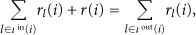
Then we explain each constraint corresponding to the flow conservation equations for multihop routing mentioned above.

• (1)

If node i is the source node which only needs to relay its own data packet, then it fulfills (2).

(2)

If node i is the intermediate node which generates and relays others' data packet, then it fulfills (3).

(3)

On the sensor node i, we have the energy consumption (4).

(4)

The length of the data collection trajectory which composed of ℜ should be constrained within L in the form of (5).

The detailed notations can be found in Table 1.

Table 1

Notation used.

ℵ	The set of sensor nodes.
Ł	The set of links.
R	The communication radius of sensor.
ℜ	The set of RPs.
${\Re }_{\text{opt}}$	The optimal set of RPs with minimum data transmission cost.
λ	The energy consumption parameter.
s	The stationary point where the Sink is located.
$C(\Re )$	The total in-network communication cost.
D	The maximum data collection delay.
T	The network lifetime.
E	The initial energy of each sensor.
L	The maximum length of ME's trajectory.
G	The adjacent matrix of the tree-shaped topology.
$Y(\Re )$	The length of trajectory composed of ℜ.
e	The energy consumption for transmitting one data packet from a node to its neighbor.
$p(i)$	The multihop transmission link between the node i and nearest RP.
$p_{\text{opt}}$	The optimal data collection trajectory with minimum data transmission cost.
$r(i)$	Data generation rate (packet/min) at node i.
$T_v$	The subtree which rooted at node v.
${\nu }_{\text{ME}}$	The average velocity of the Mobile Element.
$p_{i,j}$	The path between node i and node j.
$l(i,j)$	Wireless link between node i and node j.
$c_l(i,j)$	The ETX of link $l(i,j)\in$   Ł.
${\iota }^{\text{out}}(i)$	The sets of outgoing links at node i.
${\iota }^{\text{in}}(i)$	The sets of incoming links at node i.
$c_p(i)$	The ETX sum of the link between node i and corresponding RP, $c_p(i)={\sum }_{l\in p(i)}{c}_l$ .
${\kappa }_v$	The sum of the data rate at all the decedent nodes of v, ${\kappa }_v={\sum }_{i\in T_v}r(i)$ .
$c_{\text{save}}(p_{u,v})$	We define $c_{\text{save}}(p_{u,v})=C(u)-C(\Re )$ , where $\Re =\{u,v\}$ . This equation can be paraphrased as how many transmission count can be saved after we extend the path from node u to node v.

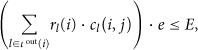
By this formulation, we implicitly assume that the data rate between any two nodes i and j (i.e., $l(i,j)$ ) is feasible under the corresponding link capacity. Our problem has an important characteristic: we should jointly consider two metrics (shown in Figure 2), Euclidean distance and ETX, in our problems. The former metric is to measure the distance covered by the ME, while the latter one is to weigh the transmission cost on each link. By doing so, we could satisfy the constraint on the length of data collection trajectory and obtain the optimization objective simultaneously.

Figure 2

Two metrics on one link: euclidean distance and ETX, respectively.

We convert the graph topology into a tree network through constructing a minimum spanning tree on the initial graph. The significance of tree network is threefold.

First, the existence of multipaths between a pair of nodes in the network always results in the problem that data packets might be trapped in a loop and cannot be delivered to the designated points [21]. We use Minimum Spanning Tree (or Steiner Tree) to avoid such problem. Second, such tree can be regarded as an initial optimization for network communication cost for it reduces the total count of ETX in terms of routing paths. Third, many applications [1, 22] are configured with fixed reporting trees when they are deployed. And such conversion can guarantee our approach to be applied in a more general case.

For case study, we take the type of Mobile Element into consideration. The intrinsic difference between these two cases is as follows: the sink is fixed at a stationary point in the first problem, but can move freely in the second problem. For the former case, the ME can be a Mobile Relay without any processing ability, and it only caches the sensing data and sends them to the stationary sink for further processing. For the latter one, sink can move freely, so the ME can be such Mobile Sink itself. Both problems have practical utilizations. For the sake of delay tolerant WSNs, employing a stationary sink and a mobile collector is relatively economical since equipping the sink with mobility results in much higher manufacturing cost and shorter allowable traversal. On the opposite, in the networks where the sensory data are urgent, it is necessary for us to adopt a Mobile Sink to satisfy with a tighter latency constraint. Figure 3 shows the difference among these two cases.

Figure 3

Illustration of two scenarios: Mobile Relay versus Mobile Sink.

5. Case  1: Rendezvous Point Selection with a Mobile Relay

In most cases, equipping the sink with mobility seems a “good” idea but lacks practical meanings, because such improvement will inevitably result in higher or even unbearable manufacturing cost and power consumption. Instead, network designers more want to let the sink locate in a stationary place and wait for the global sensing data. We facilitate this stationary sink with a Mobile Relay to collect data from RPs along a designated path, and then, the Mobile Relay uploads these data to the sink for further processing.

5.1. An Optimal Solution: RP-MR

In this part, we present an $O(n\hspace{0.17em}\text{lg}\hspace{0.17em}n)$ algorithm named Rendezvous Planning with a Mobile Relay (RP-MR) to find the optimal locations of RPs and the corresponding length-constrained data collection trajectory. The basic idea of RP-MR is to investigate which qualified trajectory (within L, passes s) retrenches the largest data transmission count of forwarding global sensing data to RPs. It can be easily proved that the path with largest data transmission count savings is the one with minimum in-network communication cost. To facilitate our algorithm, we first give three lemmas that help to construct the infrastructure of RP-MR.

Lemma 2.

Given a directed tree rooted at r, let v denote any descendent node of r, one has

$\begin{array}{c}{c}_{\text{save}}\left(p_{r,v}\right)=c_{\text{save}}\left(p_{r,\text{parent}\left(v\right)}\right)+k_v\cdot c\left(v,\text{parent}\left(v\right)\right).\end{array}$

(6)

Proof.

According to the definition of $C_{\text{save}}(p,(r,v))$ , we can develop the left part of (6) as

$\begin{array}{c}{c}_{\text{save}}\left(p_{r,v}\right)=C\left(r\right)-C\left({\mathfrak{R}}_1\right),\end{array}$

(7)

where ${\Re }_1=\{r,v\}$ .

Also, we develop the right part of (6) as

$\mathrm{\hspace{0.17em}\hspace{0.17em}}\begin{array}{cc}\hfill & c_{\text{save}}\left(p_{r,\text{parent}\left(v\right)}\right)+k_v\cdot c\left(v,\text{parent}\left(v\right)\right)\hfill \\ \hfill & \hspace{1em}\hspace{1em}=C\left(r\right)-C\left({\mathfrak{R}}_2\right)+k_v\cdot c\left(v,\text{parent}\left(v\right)\right),\hfill \end{array}$

(8)

where ${\Re }_2=\{r,\text{parent}(v)\}$ .

By (7)-(8), we have

$\mathrm{\hspace{0.17em}\hspace{0.17em}}\begin{array}{cc}\hfill & C\left({\mathfrak{R}}_2\right)-C\left({\mathfrak{R}}_1\right)-k_v\cdot c\left(v,\text{parent}\left(v\right)\right)\hfill \\ \hfill & \hspace{1em}\hspace{1em}=k_v\cdot c\left(v,\text{parent}\left(v\right)\right)-k_v\cdot c\left(v,\text{parent}\left(v\right)\right)\hfill \\ \hfill & \hspace{1em}\hspace{1em}=0,\hfill \end{array}$

(9)

where ${\Re }_1=\{r,v\}$ , ${\Re }_2=\{v,\text{parent}(v)\}$ .

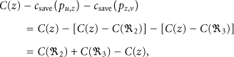
Example 3.

In Figure 4, the numbers attached to each edge indicate the ETX of links, and the numbers on the nodes denote the data generation rate. According to the definitions of $c_{\text{save}}(p_{r,\text{parent}(v)})$ and $c(v,\text{parent}(v))$ , we can calculate the following values from Figure 4:

$\begin{array}{cc}\hfill c_{\text{save}}\left(p_{r,\text{parent}\left(v\right)}\right)& =C\left(r\right)-C\left({\mathfrak{R}}^{\prime }\right)=177-149.8=27.2,\hfill \\ \hfill k_s\cdot c(s,\text{parent}\left(s\right))& =2.4\times (4+3+5)=28.8.\hfill \end{array}$

(10)

Also, we can get

$\begin{array}{cc}\hfill c_{\text{save}}\left(p_{r,s}\right)& =C\left(r\right)-C\left({\mathfrak{R}}^{\mathrm{\prime \prime }}\right)=177-121=56.\hfill \end{array}$

(11)

Thus,

$\begin{array}{cc}\hfill c_{\text{save}}\left(p_{r,s}\right)& =c_{\text{save}}\left(p_{r,\text{parent}\left(v\right)}\right)+k_s\cdot c(s,\text{parent}\left(s\right))\hfill \end{array}$

(12)

holds.

Figure 4

Illustration of a directed tree which rooted at node r, node v is derived from r.

Lemma 4.

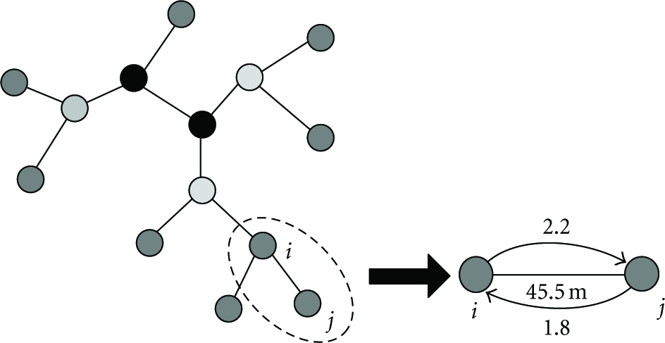
Let z denote any intermediate node on path $p_{u,v}$ , then one has

$\begin{array}{cc}\hfill C\left({\mathfrak{R}}_1\right)& =C\left(z\right)-c_{\text{save}}\left(p_{u,z}\right)-c_{\text{save}}\left(p_{z,v}\right),\hfill \end{array}$

(13)

where ${\Re }_1=\{u,v\}$ .

Proof.

We first develop the left part of (13):

$\begin{array}{cc}\hfill C\left({\mathfrak{R}}_1\right)& =C\left(u\right)-c_{\text{save}}\left(p_{u,v}\right).\hfill \end{array}$

(14)

Then, we develop the right part of (13):

$\mathrm{\hspace{0.17em}\hspace{0.17em}}\begin{array}{cc}\hfill & C\left(z\right)-c_{\text{save}}\left(p_{u,z}\right)-c_{\text{save}}\left(p_{z,v}\right)\hfill \\ \hfill & \hspace{1em}\hspace{1em}=C\left(z\right)-\left[C\left(z\right)-C\left({\mathfrak{R}}_2\right)\right]-\left[C\left(z\right)-C\left({\mathfrak{R}}_3\right)\right]\hfill \\ \hfill & \hspace{1em}\hspace{1em}=C\left({\mathfrak{R}}_2\right)+C\left({\mathfrak{R}}_3\right)-C\left(z\right),\hfill \end{array}$

(15)

where ${\Re }_2=\{u,z\},{\Re }_3=\{z,v\}$ .

Substituting the $C({\Re }_3)$ by $C(z)-c_{\text{save}}(p_{z,v})$ in (15), we have

$\mathrm{\hspace{0.17em}\hspace{0.17em}}\begin{array}{cc}\hfill & C\left({\mathfrak{R}}_2\right)+C\left({\mathfrak{R}}_3\right)-C\left(z\right)\hfill \\ \hfill & \hspace{1em}\hspace{1em}=C\left({\mathfrak{R}}_2\right)+C\left(z\right)-c_{\text{save}}\left(p_{z,v}\right)-C\left(z\right)\hfill \\ \hfill & \hspace{1em}\hspace{1em}=C\left({\mathfrak{R}}_2\right)-c_{\text{save}}\left(p_{z,v}\right).\hfill \end{array}$

(16)

By (14)–(16), we have

$\mathrm{\hspace{0.17em}\hspace{0.17em}}\begin{array}{cc}\hfill & C\left(u\right)-c_{\text{save}}\left(p_{u,v}\right)-C\left({\mathfrak{R}}_2\right)+c_{\text{save}}\left(p_{z,v}\right)\hfill \\ \hfill & \hspace{1em}\hspace{1em}=C\left(u\right)-C\left({\mathfrak{R}}_2\right)-c_{\text{save}}\left(p_{u,v}\right)+c_{\text{save}}\left(p_{z,v}\right)\hfill \\ \hfill & \hspace{1em}\hspace{1em}=c_{\text{save}}\left(p_{u,z}\right)-c_{\text{save}}\left(p_{u,v}\right)+c_{\text{save}}\left(p_{z,v}\right)\hfill \\ \hfill & \hspace{1em}\hspace{1em}=0.\hfill \end{array}$

(17)

Therefore, Lemma 4 holds.

Lemma 5.

Let v denote any node on the tree-shaped topology, then one has

$\begin{array}{c}C\left(v\right)=C\left(\text{parent}\left(v\right)\right)+c\left(v,\text{parent}\left(v\right)\right)\cdot \left({\kappa }_s-2\cdot {\kappa }_v\right).\end{array}$

(18)

Proof.

This equation is easy to understand intuitively. And the proof is quite straightforward, therefore it is omitted here.

5.2. Algorithm

In the algorithm, as all the trajectories that originate from the roots to the other vertices are different in length, we have to maintain all the trajectories starting from the root to other vertices. In the combination process (steps 7 and 8), if we do not order the paths by their length first, the time needed for finding the optimal trajectory containing the roots with length at most L is $O(n^2)$ . That is because we have to combine all pairs of paths originated from the root. But if we order the trajectories before we execute the combination process, we could find the optimal trajectory containing the roots in $O(n)$ time. To reduce the time complexity of our algorithm, here we adopt quicksort [23] to order the trajectories in $O(n\hspace{0.17em}\text{lg}\hspace{0.17em}n)$ .

Figure 5(a) illustrates the initial tree-shaped network. At step 2, we orient tree into the directed form with the root s. From step 3 to step 5, the algorithm computes $C(v)$ for each node v; at step 6, the algorithm investigates all the length-constrained (within L) trajectories; that is, in Figure 5(b), we have three trajectories within L, $s\to c$ , $s\to g$ , and $s\to f$ , respectively. At step 7, we select two trajectories found at step 6 and integrate them into a new trajectory. For instance, we operate $s\to c$ and $s\to g$ , achieve the new path $c\to s\to g$ or $g\to s\to c$ . If the length of this new trajectory is shorter than L, we regard it as a candidate path otherwise we drop it. After determining all the possible trajectories at step 6, we choose the one with maximum $c_{\text{save}}()$ from all the candidate trajectories. Then, we output the ${\Re }_{\text{opt}}$ and $C_{\text{opt}}$ . Hence, the optimal path in Figure 5(c) is $f\to s\to c$ .

Figure 5

Case study 1: an illustration of Rendezvous Point Selection with a Mobile Relay.

5.3. Theoretical Analysis of RP-MR

In this part, we state some properties of RP-MR algorithm (see Algorithm  1).

Algorithm 1: RP-MR algorithm.

(1) procedureRP-MR  $(G,L/2,s)$

(2)  Orient tree-shaped topology into a directed case with the root s;

(3)  Compute ${\kappa }_v$ for each node v using a bottom-up fashion;

(4)  Compute $C(\Re )$ in a bottom-up fashion, where $\Re =\{s\}$ ;

(5)  Compute $C(v)$ for each node v by using Lemma (6) in a top-down fashion;

(6)  Calculate the $c_{\text{save}}()$ for the trajectories (shorter than L) that originate from node s by using Lemma (6), respectively;

(7)  Combine each pair of trajectories found in Step (6). Calculating the $c_{\text{save}}()$ in the same way;

(8)  Computing the in-network data transmission cost $C({\Re }_{\text{opt}})$ for the path with maximum $c_{\text{save}}$ from the compound paths set;

(9)  return $p_{\text{opt}}$ and $C({\Re }_{\text{opt}})$ ;

(10) end procedure

Theorem 6.

The data collection trajectory $p_{\text{opt}}$ found by RP-MR is optimal.

Proof.

This theorem is easy to understand intuitively. As we have enumerated all the length-constrained trajectories and restored them in the candidate set, the optimal trajectory in the candidate set is the global optimal trajectory.

Theorem 7.

RP-MR can be done in $O(n\hspace{0.17em}\text{lg}\hspace{0.17em}n)$ .

Proof.

First, it takes $O(n)$ time to orient the tree into directed form via top-down fashion. Then we get ${\kappa }_v$ for each node v, and calculate $C(s)$ through a bottom-up traversal. In the following step, through top-down fashion, we compute the $C()$ value for each node and get the $c_{\text{save}}$ for the length-constrained trajectory by retraversing the tree in the top-down fashion. Next, we adopt quick-sort to help find the optimal trajectory with the maximum $c_{\text{save}}$ , this can be accomplished in $O(n\hspace{0.17em}\text{lg}\hspace{0.17em}n)$ . Finally, calculating the optimal $C({\Re }_{\text{opt}})$ can be done in $O(1)$ . Therefore, the time complexity of RP-MR is $O(n\hspace{0.17em}\text{lg}\hspace{0.17em}n)$ .

Theorem 8.

The data collection trajectory found by RP-MR always heads to the “hot area” in which the sensors' data generation rates are pretty high.

Proof.

This theorem can be proved by contradiction. Let $T_{h\mathrm{\hspace{0.17em}\hspace{0.17em}}a}$ denote the subtree with maximum sum of data generation rates (hot area). Suppose the optimal data collection trajectory $(p_{\text{opt}})$ does not head to $T_{h\mathrm{\hspace{0.17em}\hspace{0.17em}}a}$ . Then considering the endpoint contained in this optimal trajectory, we remove trajectory between the endpoint $p^{*}$ and the root of sub-tree $T_{h\mathrm{\hspace{0.17em}\hspace{0.17em}}a}$ , and prolong the trajectory into $T_{h\mathrm{\hspace{0.17em}\hspace{0.17em}}a}$ with same length to guarantee that the length is shorter or equal to L. According to Lemma 2, the $c_{\text{save}}$ of the new trajectory is greater than that of $p_{\text{opt}}$ . This contradicts the fact that the $p_{\text{opt}}$ is the optimal one. Therefore, the data collection trajectory found by RP-MR always heads to the “hot area”.

6. Case  2: Rendezvous Point Selection with a Mobile Sink

In this section, firstly we state the basic idea and present the pseudocode of RP-MS algorithm. Then, an execution example of RP-MS is illustrated. Finally, we evaluate the performance of RP-MS with three theorems.

Sometimes, the Sink can move inherently, that is, the Airborne Warning and Controlling System collect information from a battlefield, or the rangers with a handheld device monitors habitat area. The mobility of the sink inspires us to propose an efficient approach to deal with the case with a Mobile (unfixed) Sink.

6.1. An Optimal Solution: RP-MS

Generally, for a specific node v, the optimal trajectory either passes through node v, or lay in one of the sub-trees by removing the node v from the tree. Based on this observation, we design a recursive algorithm to find the optimal trajectory. First, the algorithm finds the optimal length-constrained trajectory which must pass through a stationary point called median (the node v with minimum $C_{\Re }$ , where $C_{\Re }=\{v\}$ ), and then, by “removing” the median, the algorithm finds the current optimal trajectory in the sub-trees which are rooted at one of median's children. In the same way, the algorithm keeps on “splitting” each sub-tree. For each sub-tree, we find the optimal length-constrained trajectory which passes through its root until every sub-tree has been examined, restoring these optimal trajectories' candidates into the candidate set. Finally, we get the global optimal one by examining the candidate set. An illustration of splitting tree technique can be found in Figure 6. In the following, we present the pseudocode of our optimal solution named Rendezvous Planning with a Mobile Sink (RP-MS) algorithm.

Figure 6

Illustration of Splitting tree technique.

6.2. Algorithm

Figure 7(a) shows the initial tree-shaped network. At step 2, RP-MS calculates $C_v$ for each node v to determine the median m. Then, it orients the network into a directed tree rooted at m, shown in Figure 7(b). Figures 7(c) and 7(d) illustrate the first iteration of finding the optimal trajectory which passes through m. The result of this process is $e\to m\to f$ (denote as $P_1$ ). At step 5, the tree splits into three sub-trees. From step 5 to step 9, it executes the optimal path in each sub-tree $P_2$ , $P_3$ , $P_4$ , respectively. Finally, we choose the global optimal path $P_{\text{opt}}$ from $P_1$ , $P_2$ , $P_3$ , $P_4$ , and the result is shown in Figure 7(f).

Figure 7

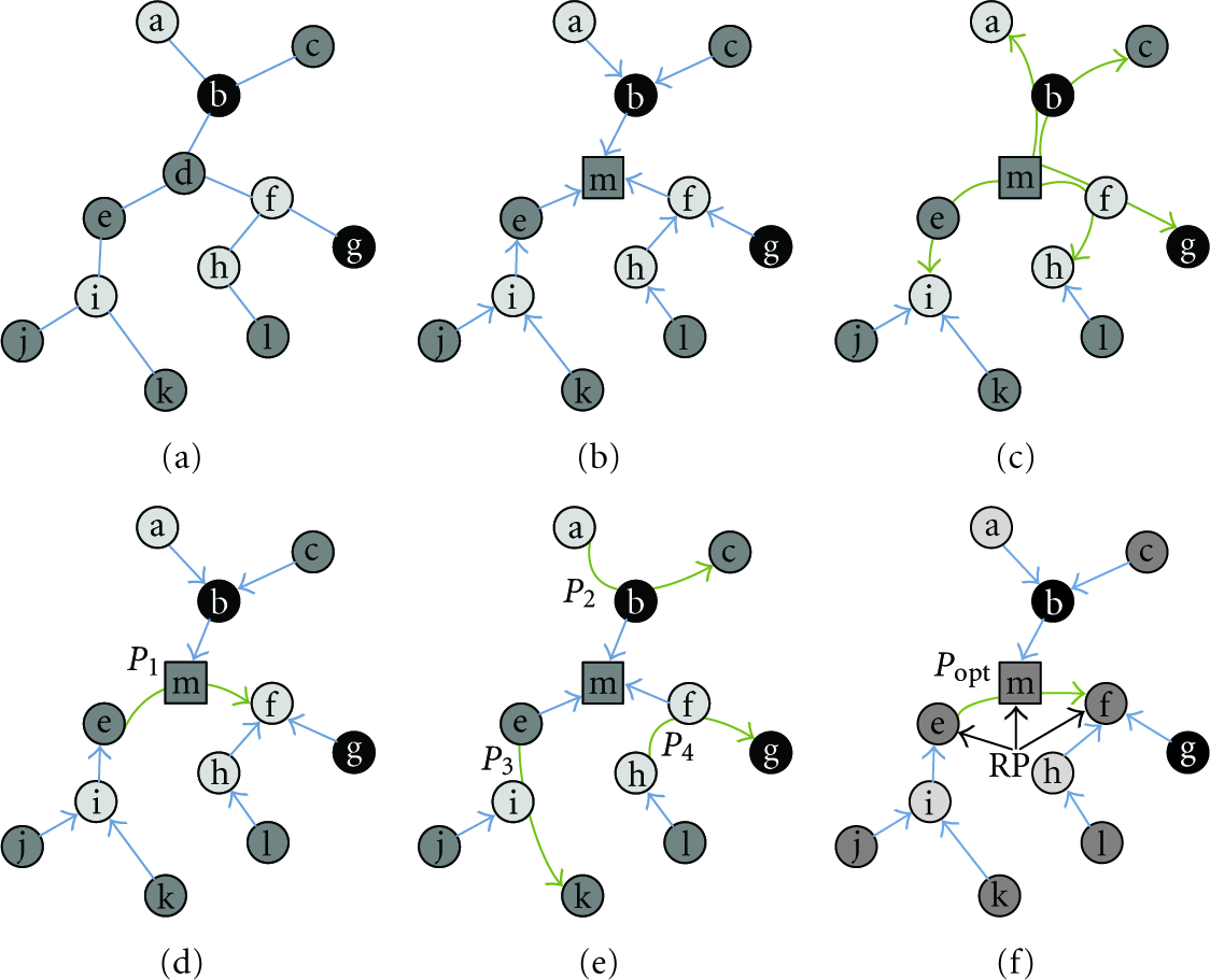
Case study 2: an illustration of Rendezvous Point Selection with a Mobile Sink.

6.3. Theoretical Analysis of RP-MS

In this part, we state some properties of RP-MS algorithm (see Algorithm  2).

Algorithm 2: RP-MS algorithm.

(1) procedure  RP-MS ( $G,L/2$ )

(2)   Find median(m) of the tree-shaped topology;

(3)   Orient tree-shaped topology into directed one which is rooted at m;

(4)   push m into queue q;

(5)   while $q\ne NULL$ do

(6)     Find the optimal trajectory $p_{\text{opt}}$ by calling RP-MR (G, L, v), where $v=q·\text{pop}()$ ;

(7)     Insert $p_{\text{opt}}$ into the candidate set SET;

(8)     Insert the children of v into queue q;

(9)   end while

(10)  Find the global optimal trajectory with minimum $C({\Re }_{\text{opt}})$ from the candidate set SET;

(11)  return   $p_{\text{opt}}$ and $C({\Re }_{\text{opt}})$ ;

(12) end procedure

Theorem 9.

Finding the median can be done in $O(n)$ .

Proof.

We divide the process of finding the median into four substeps. At step 1, we arbitrarily select a node as the root r and then orient the tree-shaped topology into a directed one. This can be achieved in $O(n)$ through Breadth-First Traversing. At step 2, we compute $C(\Re )$ in $O(n)$ with the bottom-up fashion, where $\Re =\{r\}$ . At step 3, with top-down fashion, we achieve $C(\Re )$ for each node v in $O(n)$ as well, where $\Re =\{r\}$ . Finally, we select the node with minimize $C(\Re )$ as the median in $O(n)$ . Hence, the execution time to find the median is $O(n)$ .

Theorem 10.

The data collection trajectory $p_{\text{opt}}$ found by RP-MS is optimal.

Proof.

For a given tree-shaped topology, the optimal data collection trajectory either passes through the median or be fully contained in one of the sub-trees by removing the median from the tree. As for the former case, we can easily achieve the global optimal solution in the first iteration. While for the latter case, the recursive process guarantees the optimal solution could be found. Hence, the data collection trajectory found by RP-MS is optimal.

Theorem 11.

The algorithm RP-MS finds the optimal RPs and corresponding trajectory in $O(n\hspace{0.17em}\text{l}{\text{g}}^2\hspace{0.17em}n)$ .

Proof.

As the pseudocode shows, the algorithm executes in iterative fashion. For a given level of the recursion, suppose there are k sub-trees to be examined, let $n_i$ denote the number of nodes of the ith problem. Consequently, we need $O(n_i\hspace{0.17em}\text{lg}\hspace{0.17em}{n}_i)$ time to find the current optimal trajectory. As ${\sum }_{i\in K}{n}_i\le n$ , we obtain each level of recursion in $O(n\hspace{0.17em}\text{lg}\hspace{0.17em}n)$ . Notice that the depth of the tree is $O(\text{lg}\hspace{0.17em}n)$ ; therefore we get the optimal trajectory in $O(n\hspace{0.17em}\text{l}{\text{g}}^2\hspace{0.17em}n)$ .

Theorem 12.

The data collection trajectory found by RP-MS always heads to the “hot area” as well.

Proof.

This theorem can be proved by contradiction as in Theorem 8. The proof is quite simple and is omitted here.

7. Performance Evaluation

In previous sections, we described the design techniques and important properties of our proposed algorithms. In this section, we validate the applicability and feasibility of such algorithms via comprehensive and large-scale simulations.

We evaluate the performance of RP-MR and RP-MS algorithms, and compare them with other two well-known algorithms, GREEDY and RD-VT. GREEDY is a heuristic algorithm, where the Mobile Element always moves to the nearest neighbor until the length of its path exceeds L. RD-VT is introduced by [1], where the Mobile Element's trajectory is formed by a preorder traversal of sensor nodes in the network.

7.1. Simulation Settings

We randomly deploy various number of sensor nodes on a $200\hspace{0.17em}\text{m}\times 200\hspace{0.17em}\text{m}$ square area. The transmission range of sensor is set to be 100 m, and every sensor can be chosen as a RP here. As the energy consumption of the data transmission is proportional to the ETX of corresponding link, we evaluate the energy consumption performance of various algorithms by comparing the total ETX of resulting data routing paths. All the evaluation results are averaged based on 10 different runs.

7.2. Simulation Results

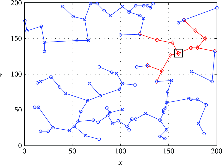
We first give the snapshot of ME's trajectory found by four algorithms in a stationary tree-shaped network, where 100 sensors are formed into a Minimum Spanning Tree. The maximum length (L) of data collection trajectory is set to be 400 m here. Figures 8, 9, 10, and 11 show the results found by GREEDY, RD-VT, RP-MR, and RP-MS, respectively. The stationary sink here is denoted by a rectangle. Clearly, the data collection trajectory in Figures 8 and 9 is limited in the top right corner in the field where less sensors are deployed. As a result, a great portion of sensors have to deliver their data to the nearest RPs via long distance transmission, which in turn, harshly increases the total in-network communication cost. In the opposite, the trajectory found by RP-MR and RP-MS is prolonged and oriented to the biggest brunch in the field, that is, the brunch in the top left and bottom left corner. Therefore, the data transmission count from each sensor to RP get fair enough, which in turn apparently reduced the in-network communication cost and verified our theorem that the data collection trajectory found by RP-MR and RP-MS always head to the hot area.

Figure 8

Data collection trajectory found by GREEDY algorithm.

Figure 9

Data collection trajectory found by RD-VT algorithm.

Figure 10

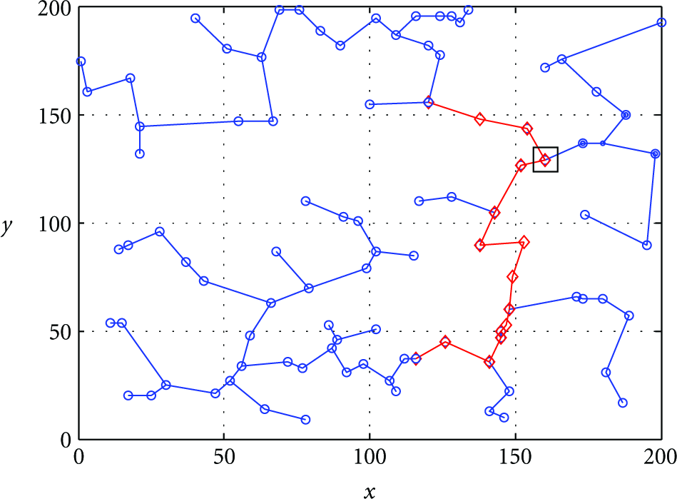
Data collection trajectory found by RP-MR algorithm.

Figure 11

Data collection trajectory found by RP-MS algorithm.

Figure 12 illustrates the relationship between the in-network communication cost of data routing paths and the length of Mobile Element's trajectory. 300 sensor nodes are randomly deployed in the field. All algorithms' performance becomes better when the ME mobility increases. Consistent with the result in Figure 12, our algorithms are superior to other two competitors. Specifically, the gap between RP-MR and RP-MS decreases with the rise of the length of the trajectory. This implies that when the length of data collection trajectory is chosen properly, the result yield by RP-MR stays in the same level of the result acquired by RP-MS in terms of in-network transmission cost. In contrast, GREEDY and RD-VT achieves similar result which almost triple the result of RP-MR and RP-MS under the same settings, which implies that the network can enjoy a longer lifetime in RP-MR and RP-MS compared with other two algorithms.

Figure 12

In-network communication cost versus length of data collection trajectory L.

Figure 13 shows the relationship between the maximum work load among RPs and the length of the ME's trajectory. Similar to Figure 12, 300 sensor nodes are randomly deployed in the field as well. According to Figure 13, the maximum work load incurred by four algorithms all decrease with the increase of L. More specifically, when the ME trajectory is short, the maximum work load is extremely heavy in GREEDY (2300), RD-VT (2000), RP-MR (1100), and RP-MS (1000). However, as L increases, RP-MR and RP-MS rapidly decreases its maximum work load, and the gaps between them are largely narrowed. This implies that both of our proposed algorithms can effectively mitigate the work load on the bottleneck RP. Although the same trend can be found in the result achieved by GREEDY and RD-VT, they still stay in a high level with respect to the work load, which implies that the network cannot be prolonged effectively.

Figure 13

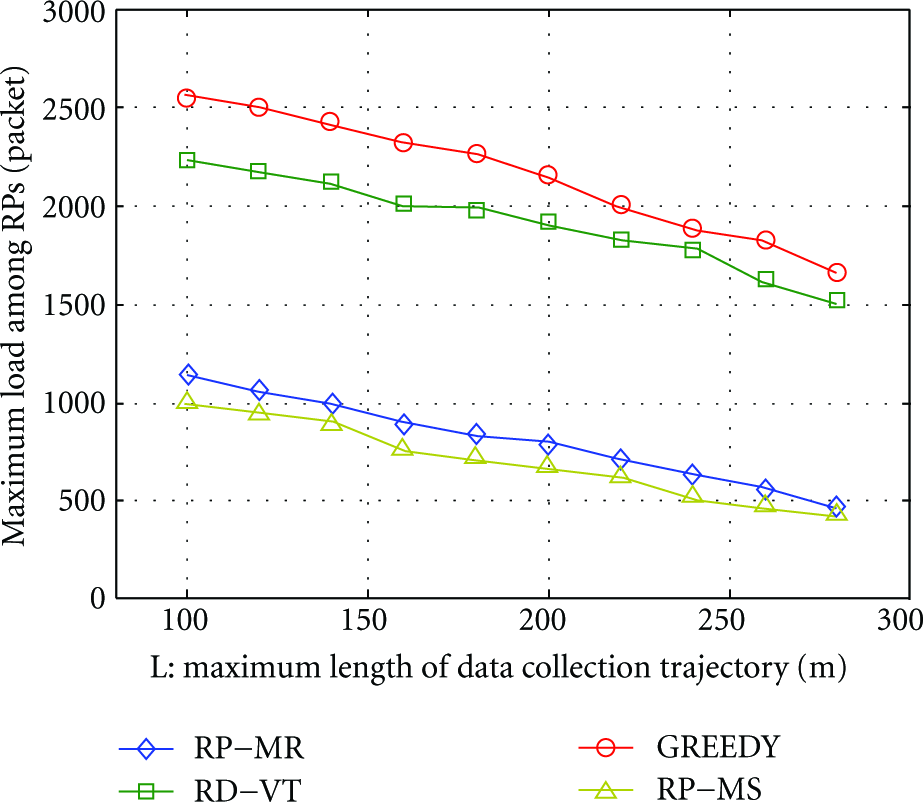
Maximum load among RPs versus length of data collection trajectory L.

Figure 14 compares the in-network communication cost of resulting data routing paths formed by different algorithms with the number of source nodes. The mobile sink trajectory length L is 400 m. Figure 14 illustrates that RP-MR and RP-MS both outperform GREEDY and RD-VT. Compared with the RP-MS where the Mobile Element can move freely, its counterpart RP-MR also works well, with only a slight performance distortion in terms of the data transmission cost. In addition, the gap from GREEDY or RD-VT to RP-MS or RP-MR increases as more sensor nodes are involved. It indicates that RP-MR and RP-MS can effectively reduce the energy consumption by taking advantage of the property that the optimal trajectory always heads to the largest brunch, that is, “hot area”.

Figure 14

In-network communication cost versus number of sensor nodes.

Figure 15 compares the maximum work load among RPs incurred by different algorithms with the number of sensor nodes. Same to Figure 14, the ME trajectory length L is set to be 400 m as well. According to Figure 15, all of the maximum work load among RPs generated by the four algorithms increase with the number of sensors. Specifically, the curves of GREEDY and RD-VT change rapidly with the increase of sensor nodes, while the curves composed of RP-MR and RP-MS increase smoothly. This is an indication of the effectiveness of RP-MR and RP-MS to prolong the network lifetime since the RP always drain its energy first among the sensor nodes and paralyze the network. Besides, the gap between RP-MR and RP-MS aggrandized gradually, which indicates that RP-MS is superior to RP-MR in terms of prolonging the network lifetime.

Figure 15

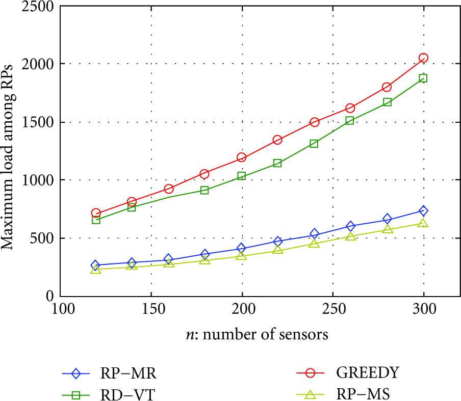
Maximum load among RPs versus number of sensor nodes.

8. Conclusion

In this paper, we study the rendezvous data collection problem for the Mobile Element (ME) in heterogeneous sensor networks where data generation rates of sensors are distinct. Essentially different from previous works, the link quality is assumed instable and the sensory data cannot be aggregated in our paper. Such assumptions highlight the dynamic properties of WSNs and tend to be more practical. We introduce to optimize the energy consumption on gathering the global data. By doing so, the Mobile Element is able to efficiently collect network-wide data within a given delay bound meanwhile the network eliminates the energy bottleneck to prolong its lifetime. Then we give two algorithms for dealing with different rendezvous data collection scenarios. In the Mobile Relay scenario where the ME's trajectory must pass through a given point to upload sensory data, an $O(n\hspace{0.17em}\text{lg}\hspace{0.17em}n)$ algorithm named RP-MR is proposed to approach the optimal solution: (1) the optimal Rendezvous Points (RPs) to collect global sensory data; (2) the optimal data collection trajectory for the Mobile Relay to gather the cached data from RPs and upload to a fixed point, that is, the sink, for further processing. In the latter case where the Mobile Element can process the sensory on its motion, that is, Mobile Sink, we develop an $O(n\hspace{0.17em}\text{l}{\text{g}}^2\hspace{0.17em}n)$ algorithm named RP-MS to recursively investigate the optimal solution. We prove the correctness of our proposals both in theoretical analysis and extensive simulations.

A possible future work is to further optimize the data collection trajectory. In the case studies of this work, we implicitly assume that the Mobile Element must walk along the edges of the tree. Actually, instead of traversing each RP, the ME needs only one step in the data transmission range of the RPs. By doing so, the length of data collection trajectory is retrenched. Therefore we could find more RPs and further minimize the in-network communication cost than the approaches before.