A Distributed Reclustering Hierarchy Routing Protocol Using Social Welfare in Wireless Sensor Networks

Abstract

In recent years, there has been a rapid proliferation of research concerning Wireless Sensor Networks (WSNs), due to the wide range of potential applications that they can be used for. Lifetime is one of the most important considerations for WSNs due to their inherent energy constraints, and various protocols have been proposed to overcome these difficulties. This study proposes a novel distributed reclustering routing protocol: Predictive and Adaptive Routing Protocol using Energy Welfare (PARPEW). PARPEW incorporates the concept of energy welfare (EW) to achieve both energy efficiency and energy balance simultaneously. PARPEW is equipped with a cluster head (CH) shift mechanism that utilizes predictive energy after transmission for the computation of EW. The average case time complexity of the shift mechanism belongs to $O({|C|}^2)$ , where $|C|$ is the average number of sensors in a cluster in the WSN. Experimental results demonstrate that the new protocol is capable of significantly prolonging the lifetime of WSNs under various scenarios.

1. Introduction

Wireless Sensor Networks (WSNs) are capable of sensing physical or environmental conditions, such as motion, pressure, and images of the environment, as well as seismic, electromagnetic, and acoustic waves. Sensor nodes form an ad hoc network within the target field, routing data packets to a specified center(s). For example, sensors distributed in a forest can send signals to the administrator, which in turn raises an alarm in the event of a fire. WSNs were originally motivated by military applications to detect dangerous situations, such as attack detection and battlefield surveillance. Recently, WSNs have attracted attention for a wider range of compelling potential applications [1–3], including traffic monitoring, environmental (indoor and outdoor) monitoring, logistical support, human-centric applications, such as healthcare [4], and applications in industrial automation [5, 6].

One notable attribute of wireless sensors is their need to operate with limited resources, resulting in difficulties that include recharging batteries, low computational capability, and narrow communications bandwidth. After exhausting their energy supply, sensors are no longer able to execute tasks, making energy efficiency one of the most important issues in WSN research. Routing is the method by which sensors gather and process data, select the transmission path, and relay data packets to the base stations (BSs), and has been shown to significantly impact the energy efficiency and consequently the lifetime of WSNs [7–9]. Numerous routing protocols have been proposed; however, due to energy considerations, multihop forwarding is the only option in most situations. Unfortunately, deploying a large number of sensors complicates the routing problem, making the pursuit of a centralized algorithm impractical. Distributed protocols for WSNs are far more scalable than their centralized counterparts, enabling them to operate efficiently in large-scale sensor networks. Thus, most current research is focused on distributed routing.

In this paper, our main focus is on distributed cluster-based routing protocols [7–11]. One of the primary methods that have been widely used to increase the lifetime of WSNs and achieve network scalability is clustering. Clustering, often referred as “grouping” in the early literature, has proven to be a key technique for efficiently managing WSNs [11, 12]. However, clustering in WSNs presents several challenges, as described below.

• (1)

To balance the energy consumption of the sensors, it is necessary to rotate the role of the cluster heads (CHs) among them.

(2)

The number of clusters must be adjusted according to several factors, including the current network topology and the residual energy of the sensors.

(3)

Sensors should not expend excessive energy on intracluster communications.

In this research, we propose a novel cluster-based routing protocol based on the concept of social welfare as used in economics to manage the requirements described above. Social welfare simultaneously measures the energy efficiency and energy balance of the WSN and transfers the role of the CHs to more appropriate nodes. The proposed protocol is simple, distributed, and self-organized, and simulation results demonstrated a global extension of the lifetime of the WSN under a variety of scenarios.

The remainder of this paper is organized as follows: in Section 2 we review recently proposed cluster-based routing protocols; Section 3 describes the system model. Section 4 introduces the social welfare function and presents our proposed routing protocol. Section 5 evaluates the performance of our routing protocol in comparison with LEACH and LEACH-C. The final section presents our conclusions and plans for future work.

2. Literature Review

Younis et al. [10] surveyed various classes of WSN clustering techniques and pointed out two key issues involved with those techniques: the parameter(s) used for selecting CHs; and the nature of cluster protocols (iterative or probabilistic). Reference [11] surveyed the rules of CH selection in clustering protocols for WSNs. Based on their classification system, CH selection strategies can be categorized into deterministic, adaptive, and combined schemes. In deterministic schemes, the fixed attributes of a sensor, such as node degree or node ID, are used to determine their roles. In adaptive schemes, the dynamic information of a sensor or its surroundings, such as residual energy, are taken into consideration. Based on the parameters considered, adaptive schemes can be further subdivided into fixed parameter probabilistic schemes and resource adaptive probabilistic schemes. A combined scheme is any protocol which uses the combined characteristics of deterministic and adaptive schemes.

Heinzelman et al. [12] developed the original clustering protocol: Low-Energy Adaptive Clustering Hierarchy (LEACH). The operation of LEACH is divided into rounds beginning with a setup (or advertisement) phase. The decision to become a CH is made by each node through the selection of a random number between 0 and 1. If the number is less than the threshold $T(n)$ , the node becomes a CH for the current round. The threshold is set as

$T\left(n\right)=\{\begin{array}{cc}\frac{p}{1-p\cdot \left(r\cdot \mathrm{mod}\left(1/p\right)\right)},\hfill & \text{if}\hspace{0.17em}\hspace{0.17em}n\in G,\hfill \\ 0\hfill & \text{otherwise},\hfill \end{array}$

(1)

where p is a parameter representing the desired percentage of CHs, and G is the set of nodes that have not been CHs during last $1/p$ rounds; r is the current round number. Self-selected CHs broadcast their decisions to all nodes, and the normal (non-CH) nodes determine which clusters to join based on distance. After the clusters are organized, each CH node receives all of the data packets from the other nodes in its cluster. It then compresses, fuses, and aggregates the data before sending it on to the base station. LEACH-Centralized (LEACH-C) is a centralized version of LEACH, proposed by Heinzelman et al. [13], which forms optimal clusters by communicating with the base station and using location-tracking methods such as GPS. In the setup phase, every node sends a broadcast packet that includes its residual energy and location to the base station. The base station runs a Simulated Annealing (SA) algorithm to select CHs and cluster formation and then broadcasts a message indicating the CH ID for each node. The remaining phases of LEACH-C are identical to those of LEACH. The optimal clustering procedure is performed in each round. When the protocol for optimal clustering is executed efficiently, the lifetime of the WSN can be increased significantly. Other variants of LEACH are described in [14, 15].

Two hierarchical routing protocols, called TEEN and APTEEN, were proposed in [16, 17], respectively. TEEN is a hierarchical cluster routing protocol, very similar to LEACH, which senses the medium, switches on the sensors and transmitters, and sends data periodically. In TEEN, however, two parameters, called soft threshold and hard threshold, are set to limit how frequently data is transmitted. Following the cluster formation phase, a CH sends its members the hard threshold and soft threshold values. Only sensors which satisfy the following two conditions can switch on their transmitters and transmit their data to their CHs: the current sensing value must be greater than the hard threshold; the difference between the current sensing value and the last sensed value must be equal to or greater than the soft threshold. The major drawback of TEEN is that nodes are never able to send data if the thresholds are not reached. Therefore, the thresholds must be correctly set by applications and users must accept a tradeoff between data accuracy and energy consumption. On the other hand, in APTEEN the CHs first broadcast a number of application-oriented parameters, including attributes, thresholds, schedule, and count time. Attributes are a set of physical parameters for which users would like to obtain data. Thresholds include both the hard and soft types. Count time is the maximum difference in time between two successive transmissions sent by a node. The main breakthrough in APTEEN is that a node is forced to turn on its transmitter and retransmit the data if it does not successfully transmit the data in a period of time equal to the count time. APTEEN resolves the problem of data accuracy while flexibility is provided by the count time.

In HEED [18], each node joins only one cluster and communicates directly with its CH. In the beginning, a predefined proportion, $C_{\text{prob}}$ , of sensors create the initial CH announcements. Unlike LEACH, which randomly chooses CHs, a sensor with high residual energies has a higher probability of being a CH using the following equation: ${\text{CH}}_{\text{prob}}=C_{\text{prob}}·(E_{\text{residual}}/E_{\max \hspace{0.17em}})$ , where $E_{\max \hspace{0.17em}}$ is the maximum amount of energy, and $E_{\text{residual}}$ is the residual energy of the sensor. HEED then enters a repetition phase. During this phase, each sensor repeats a fixed number of iterations until it joins one cluster in which the CH is in its least transmission range. If a sensor receives no announcement from a CH, it designates itself a CH and broadcasts an announcement of its status. At the end of each iteration, each sensor node doubles its CH_prob and repeats the iteration. The repetition phase generates two results: if CH_prob is more than 1, the sensor becomes a final CH; if CH_prob is less than 1, the sensor becomes a tentative CH that can become a regular node if it finds another CH with a lower energy cost.

In [19], the authors proposed a distributed protocol for assigning sensors to clusters. Each sensor is equipped with an absolute timer using a random waiting time and neighborhood information to decide whether to join an existing cluster or to form its own cluster. Reference [20] proposed two distributed algorithms for CHs selection: ACE-C and ACE-L. The former uses counting to ensure that the sensor networks have the same number of clusters, while the latter uses the location information to select the CHs. The authors set a number of fixed reference points in the observed area, so that the sensors closest to those reference points would be selected as CHs. Other cluster-routing techniques developed in recent years include [21–26].

3. System Model

3.1. Preliminaries: Definitions and Notations

A set of sensors, S, is distributed in a target area and a base station collects data from them. Each sensor node is equipped with a nonreplenishable battery. $e_i^0$ is the initial energy of sensor i; $e_i^t$ denotes the residual energy of sensor i at round t. If all of the sensors are homogeneous, $e_i^0$ can be simplified to $e^0$ .

In the literature, the lifetime represents the main performance measure of WSNs. The most common definition of a WSN lifetime is the period of time until a portion of sensor nodes die during operation as a result of energy depletion. The threshold varies depending on what application the WSN is being used for [27]. The most common metric is the number of time periods it takes until the first sensor node dies. This is a pessimistic approach because the remaining sensors may still provide adequate service. Coverage is another indicator of lifetime which is defined as the number of time periods until the coverage is reduced to a set percentage of area. We use the so-called Disk model [28], which refers to the range within which a sensor can detect an event with certainty.

In our model, a base station is required to collect data periodically from the entire network. In every round, the sensors aggregate clusters and report the data to the base station through CHs in the sensor network. We call this a clustering data gathering sensor network. Our objective is to find a clustering strategy that provides a sensor network with the optimal lifetime.

In the next section, we introduce the radio model which is used to compute the energy cost.

3.2. Radio Model

In this example, we use the first order radio model introduced in [13]. In this model, a typical sensor consists of seven components as shown in Figure 1: receiver antenna, receive electronics, sensor, data processor, two transmit electronics, and transmitter antenna. We take into account three major energy consuming operations: transmission, reception and compression. In order to transmit a μ-bit message from sensor i to sensor j over a distance $d_{ij}$ , the radio model is formulated as follows:

$\begin{array}{cc}\hfill E_{\text{TX}}\left(\mu ,d_{ij}\right)& =E_{\text{TX}}\left(\mu \right)+E_{\text{AMP}}\left(\mu ,d_{ij}\right)\hfill \\ \hfill & ={\varepsilon }_{\text{tx}}\cdot \mu +{\varepsilon }_{\text{amp}}\cdot \mu \cdot d_{ij}^2,\hfill \end{array}$

(2)

where $E_{\text{TX}}(\mu ,d_{ij})$ denotes the total energy dissipated in the transmission. In a successful μ-bit transmission, the sensor consumes $E_{\text{TX}}(\mu )$ to run the transmitter circuitry and $E_{\text{AMP}}(\mu ,d_{ij})$ for the transmitter amplifier. ${\varepsilon }_{\text{tx}}$ is the one bit of energy consumed by the transmitter electronic components and ${\varepsilon }_{\text{amp}}$ is an amplifier characteristic constant. $d^2$ is energy loss due to channel transmission which approximates the free-space propagation model. To receive the μ-bit message, the energy cost of the sensor is

$\begin{array}{c}{E}_{\text{RX}}\left(\mu \right)={\varepsilon }_{\text{rx}}\cdot \mu ,\end{array}$

(3)

where $E_{\text{RX}}(\mu )$ is the energy consumed when the sensor receives the μ-bit message. The parameters ( ${\varepsilon }_{\text{tx}}$ , ${\varepsilon }_{\text{rx}}$ , and ${\varepsilon }_{\text{amp}}$ ) depend on several factors such as the design of the radio, and space conditions.

Figure 1

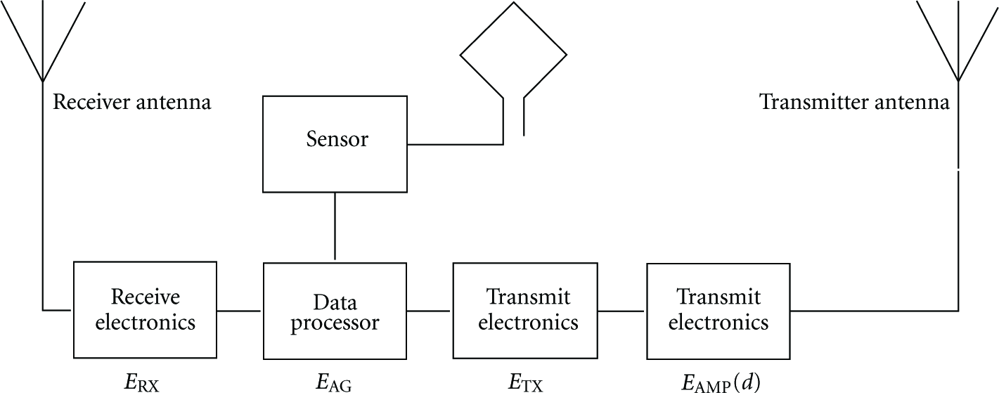
The major components of a typical sensor.

The third source of energy consumption is the data aggregation performed by each CH. The aggregation not only eliminates data redundancy, but also merges data packets and reduces the number of transmissions to the base station. The single aggregation functions are MAX and MIN. For example, if we wanted to know the highest temperature in the target area in a supervisory application, the MAX function would be suitable for that purpose. Figure 2 shows an example of routing the MAX temperature to the base station. The number beside each node represents the local temperature; the numbers in parentheses signify the maximum value after data aggregation. In our model, we refer to the energy consumed for compressing a bit of data as ${\varepsilon }_{\text{ag}}$ and the total energy dissipated for compressing $n·\mu$ bits is $E_{\text{AG}}$ :

$\begin{array}{c}{E}_{\text{AG}}\left(n,\mu \right)={\varepsilon }_{\text{ag}}\cdot \left(n\cdot \mu \right),\end{array}$

(4)

where n is the number of packets as well as the number of sensors in the cluster ( $n-1$ packets are sent to the CH and the CH itself also generates one data packet), and μ is the number of single data packets received. Note that only CHs need to expend $E_{\text{AG}}(n,\mu )$ .

Figure 2

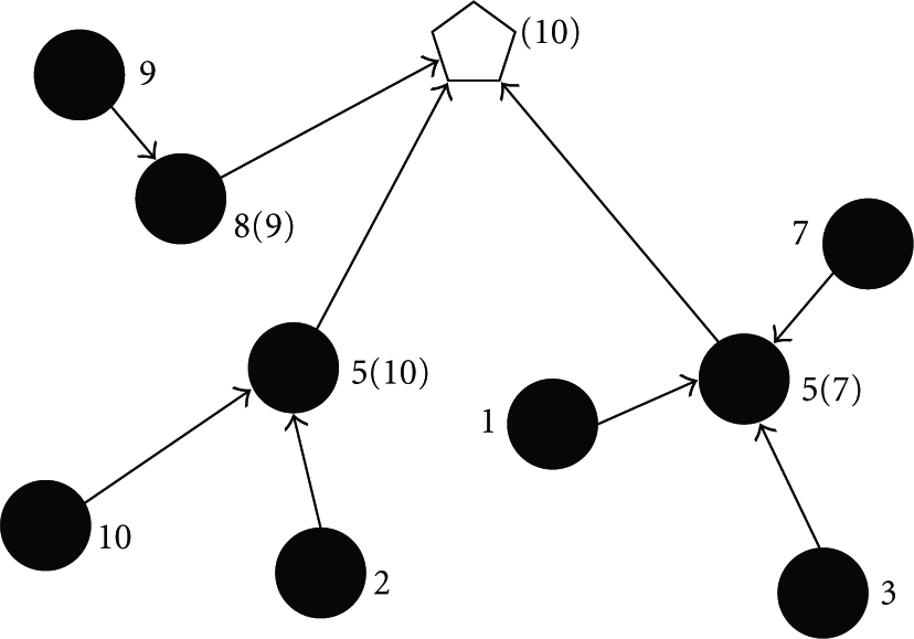
Data aggregation using the MAX function.

3.3. Assumptions

To clarify the model under consideration, we make similar assumptions to previous work [12, 18, 19, 29] as follows.

• (1)

Each sensor has a unique predefined ID that is attached to the end of each data packet and used to identify the source.

(2)

A stationary base station is located away from the target area and has no energy limitations.

(3)

If not specifically mentioned, all sensors in the sensor network are homogeneous, which means they all have the same sensing radius and the same initial energy $e^0$ .

(4)

The WSN is proactive, in which every node generates the same amount of data periodically; in other words, the size of the data packet does not depend on the condition of the sensors or the surroundings.

(5)

Each sensor can adjust its transmission range to use the minimum amount of energy required to reach the intended next hop sensor in the network including the base station. As a result, the transmission energy consumption depends on the distance between the source sensor and the next hop sensor.

(6)

Each sensor is fixed. It is not necessary for each sensor to know its own location, but the distance matrix among sensors is necessary for our algorithm. In this research, we may require Global Positioning System (GPS) equipped sensors or some non-GPS techniques to obtain the distance matrix of the sensors. This can be computed according to the intensity of electromagnetic waves and an accurate clock in each sensor, or by the triangulation method.

(7)

We assume ideal transmission conditions among communication nodes. In other words, every data packet is successfully transmitted to its destination. This assumption also means that all of the transmissions are scheduled (via the time slot method or by multifrequency broadcasting), so that the messages are not interfered with. This assumption requires a perfect MAC layer condition. In this paper we only discuss the routing problem; determining how to achieve a perfect MAC layer condition is beyond the scope of the study.

(8)

Only CHs can transmit data packets to the base station and only CHs can compress data. We do not address any specific aggregation function, but we use something similar to the MAX function. This means that the number of output packets is the same no matter how many input data packets there are.

To sum up, these assumptions simulate a stationary homogeneous WSN with one BS, and its applications require continuous data collection, whereby each live sensor has to transmit a data packet each round. Although this first order radio model is a simplified model, it fits the practical results found in the real world. Moreover, the radio model can change its parameters and is adaptable to different sensor hardware platforms.

4. Predictive and Adaptive Routing Protocol Using Energy Welfare (PARPEW)

4.1. Energy Welfare Function

As stated in Section 2, there are several requirements for designing a WSN routing protocol. The most challenging issue is prolonging the lifetime of the WSN by simultaneously achieving high energy efficiency and energy balance. To address this issue, we introduce a function usually used by social scientists to judge a society's welfare income. The welfare function $W_{A(\alpha )}$ is called the Atkinson welfare function and is computed as follows [30]:

$\begin{array}{c}{I}_A\left(\alpha \right)=1-{\left[\frac{1}{n}{\displaystyle \sum }_{a\in A}{\left(\frac{P_a}{\bar{P}}\right)}^{1-\alpha }\right]}^{1/\left(1-\alpha \right)},\\ W_A\left(\alpha \right)=\bar{P}\left(1-I_{A\left(\alpha \right)}\right),\end{array}$

(5)

where $I_{A(\alpha )}$ is the Atkinson index; A is a set of people in a population; n is the number of people in the population; $P_a$ is the income of person a in the population; and $\bar{P}$ is the average income of the population. When $\alpha =1$ , the Atkinson welfare function is defined as

$\begin{array}{c}{e}^{\left(1/n\right){\sum }_{a\in A}^{}\ln P_a}.\end{array}$

(6)

α is called an inequality aversion parameter, which signifies the strength of society's penalty for inequality, and usually ranges from 1.5 to 2.5 [31]. As α approaches zero, $I_{A(0)}$ becomes zero, which means that no punishment imposed for the inequality. As α increases, greater penalties for inequality are imposed.

The social welfare function is used to compute the predictive energy welfare (EW) of cluster C at round t to simultaneously measure energy efficiency and energy balance according to the following formula:

$\begin{array}{c}{I}_C^t\left(\alpha \right)=1-{\left[\frac{1}{\left|C\right|}{\displaystyle \sum }_{i\in C}{\left(\frac{e_i^t}{{\bar{e}}^t}\right)}^{1-\alpha }\right]}^{1/\left(1-\alpha \right)},\\ {\text{EW}}_C^t\left(\alpha \right)={\bar{e}}^t\cdot \left(1-I_C^t\left(\alpha \right)\right)={\left[\frac{1}{\left|C\right|}{\displaystyle \sum }_{i\in C}{\left(e_i^t\right)}^{1-\alpha }\right]}^{1/\left(1-\alpha \right)},\end{array}$

(7)

where ${\bar{e}}^t$ is the average energy residual of the sensors in C, at round t, and $|C|$ is the number of sensors in C. The weight between the average and equality is now determined through aversion parameter α. Note that we would like to have a higher EW value in every round because both energy efficiency and energy balance are important to prolong the lifetime of the WSN.

4.2. Energy Welfare Example

Before proceeding to our protocol, we provide the following example to better understand the use of the social welfare function. There are three sensor nodes in a cluster as shown in Figure 3(a). In this example only transmission and reception energy consumption is considered. For the sake of simplicity, we assume that a CH must expend 1 unit of energy for reception. Figure 3(a) shows the energy consumption for transmission among sensors. The initial energy levels of the three sensor nodes (e.g., $E_{\text{TX}}(\mathrm{2,1})$ indicate the transmission energy between nodes 2 and 1; while $e_1^0$ refers to the initial energy of node 1). We now define the Energy After Transmission (EAT), in which ${\text{eat}}_i^t$ of sensor i at round t is the predictive residual energy after transmission and reception of data. As a result, the EW of the cluster $C_k^t$ at round t can be defined as

$\begin{array}{c}{\text{EW}}_{C_k^t}\left(\alpha \right)={\left[\frac{1}{\left|C_k^t\right|}{\displaystyle \sum }_{i\in C_k^t}{\left({\text{eat}}_i^t\right)}^{1-\alpha }\right]}^{1/\left(1-\alpha \right)}.\end{array}$

(8)

Figure 3(b) shows the sensor and EW energy residuals after transmission that resulted from the selection of each alterative CH. For example, if we choose node 1 as the CH and uses α as 1.5 for calculating EW (we call the index of this cluster the first cluster; $h_1=1$ means that the CH of the first cluster, $h_1$ , is sensor 1), then

$\begin{array}{cc}\hfill & {\hspace{0.17em}{\text{EW}}_{C_1^t}\left(\alpha =1.5\right)|}_{h_1=1}\hfill \\ \hfill & \hspace{1em}\hspace{1em}={\left[\frac{1}{3}\cdot \left(16^{(1-1.5)}+49^{(1-1.5)}+24^{(1-1.5)}\right)\right]}^{1/(1-1.5)}\hfill \\ \hfill & \hspace{1em}\hspace{1em}\approxeq 25.25.\hfill \end{array}$

(9)

It is clear that although the highest average residual energy is obtained when node 3 is selected as the CH (the average residual energy is 30.33), EW influences the cluster to select node 2 as a CH which results in a higher EW ( $\text{EW}=28.66$ ). Note that the function has the inequality aversion parameter, α. The flexibility provided by the aversion parameter is an important factor that can be used to accommodate various WSN applications.

Figure 3

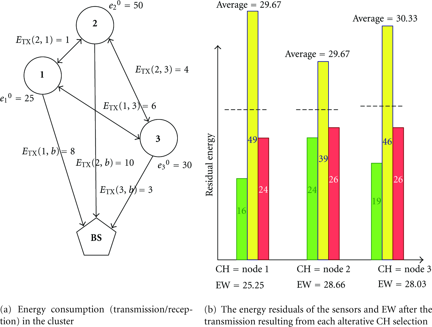
An example to illustrate EW.

4.3. PARPEW Details

Predictive and Adaptive Routing Protocol using Energy Welfare (PARPEW) is a distributed cluster-based protocol that performs local data collection and routing decisions by evaluating the EW. PARPEW operates in each round in two stages: the cluster setup stage; and steady-state stage. In the cluster setup stage, clusters are formed and CHs are selected. In the steady-state stage, sensors collect data and send it to their corresponding CHs. The CHs then aggregate the data and transfer it to the base station.

During operation, the role of sensor i ( ${\mathit{\text{role}}}_i$ ) can be in one of four different states: normal node (normal), temporal CH (tempCH), real CH (realCH), and dead node (dead). Figure 4 shows the transition diagram of a sensor as follows.

• (i)

Normal node: an active sensor that does not have any representative role for a cluster. Nonetheless, a normal node can be selected as a temporal or real CH.

(ii)

Temporal CH: the role of a temporal CH is to gather information (residual energy) from all members of the same cluster and determine the real CH based on the EW.

(iii)

Real CH: the role of a real CH is to collect data from all members of the same cluster, aggregate and compress the data, and forward it to the base station.

(iv)

Dead node: when a node's energy is depleted, it becomes a dead node and does not perform any operations.

Figure 4

Sensor state transition diagram.

Initially, a one-time operation is performed to determine the distance matrix: the BS broadcasts the TDMA schedule to the nodes; each node broadcasts the control packet to every other node according to the time slots in the TDMA schedule; each node obtains the relative distance matrix either by estimating the time delay, or through the attenuation of electromagnetic waves, or simply via GPS. The nodes then store the distance matrix in their memory.

Operational details regarding PARPEW are provided in Algorithms 1–3. We illustrate the four phases that comprise the cluster setup stage. At the beginning of each round, the base station starts the round and broadcasts the TDMA schedule to every node. The TDMA schedule specifies the time slots assigned to each live node to avoid packet collision in the cluster setup stage.

• (i)

Advertisement Phase. At the beginning of every round, each node attempts to selects itself as a temporal CH by generating a random number between 0 and 1 (Algorithm 1, Line 3). If the random number is less than, or equal to, a given parameter, p, the node becomes a temporal CH and then broadcasts a message (the first control packet, $C{P}_1$ ) containing its ID (Algorithm 1, Lines 4-5); otherwise, the node is considered a normal node and must wait for control packets from temporal CHs.

(ii)

Cluster Formation Phase. Once the nodes have selected themselves as temporal CHs, the remaining normal nodes must determine which clusters they belong to. The decision is based on the signal strengths of the control packets received from the temporal CHs. A normal node becomes a member of the CH with the highest signal strength (i.e., the closest CH; Algorithm 2, Lines 2–8). After each node determines which cluster it belongs to, it sends a the second control packet ( $C{P}_2$ ) containing its residual energy and ID to its temporal CH (Algorithm 1, Line 11).

(iii)

Real CH Selection Phase. Once clusters have been formed, temporal CHs determine real CHs by means of EW (Algorithm 1, Lines 13-14). The decision is expressed by

$\underset{i\in C_k^t}{\arg \hspace{0.17em}\max }{{\text{EW}}_{C_k^t}\left(\alpha \right)|}_{h_k=i},$

(10)

${\text{EW}}_{C_k^t}(\alpha ){|}_{h_k=i}$ is the predicted EW value of the kth cluster if sensor i is selected as the CH (Algorithm 3). First, the temporal CH computes all possible EATs if each member of its cluster is selected to be the real CH (Algorithm 3, Lines 9–11). It then uses those EATs to compute the best one to become the CH based on the maximum EW method (Algorithm 3, Lines 12–20). The sensors that are not selected to be the real CH revert to normal nodes (Algorithm 3, Lines 21–27). As previously mentioned, distances among members in a cluster and the distance to the base station can be determined through a number of non-GPS techniques.

(iv)

Schedule Creation Phase (Algorithm 1, Lines 15–17). The temporal CH creates and distributes to the members of its cluster an information packet that contains the TDMA schedule and the ID of the real CH. The TDMA schedule specifies the time slots assigned to each member in the cluster. The normal nodes send their data to the real CH within the assigned time slots specified in the TDMA schedule.

Algorithm 1: Cluster setup stage algorithm in PARPEW.

(1) procedure MAIN(i)     ⊳ for every node $i\in S$

(2)   ${\mathit{\text{role}}}_i\leftarrow \varnothing$ ;           ⊳ Initialize

( $3)$   if   $\mathit{\text{rand}}()\le p$   then

(4)    ${\mathit{\text{role}}}_i\leftarrow \mathit{\text{tempCH}}$

(5)   Broadcast the control packet $C{P}_1$

(6)  else

(7)    ${\mathit{\text{role}}}_i\leftarrow \mathit{\text{Normal}}$

(8)    $m\leftarrow$ ReceivesControlPackets (i,   $C{P}_1$ )

(9)   end  if

(10)   if   ${\mathit{\text{role}}}_i=\mathit{\text{normal}}$    then

(11)   Send the control packet $C{P}_2$ to node m

(12)  else            $⊳{\mathit{\text{role}}}_i$ = $\mathit{\text{tempCH}}$

(13)   ReceivesControlPacket (i, $C{P}_2$ )

(14)    $\mathit{\text{role}}[j]\leftarrow$   ComputeEW()  $⊳j\in \hspace{0.17em}\hspace{0.17em}{C}_k^t$ , including i

(15)   Schedule and send    $C{P}_3$ to nodes in $C_k^t$

(16)  end  if

(17) ReceivesControlPacket (i, $C{P}_3$ )

(18)  Enter Steady-state stage

(19) end  procedure

Algorithm 2: Code snipper of receives control packets function.

(1) procedure  RECEIVES CONTROL PACKETS (i,CP)

(2)  if $CP={CP}_1$   then

(3)   if   ${\mathit{\text{role}}}_i=\mathit{\text{tempCH}}$   then

(4)    Dispose $C{P}_1$

(5)   else      ⊳ if node i is a normal node

(6)      $m\leftarrow {\arg \hspace{0.17em}\max \hspace{0.17em}}_{j\in S}\hspace{0.17em}C{P}_1·{\mathit{\text{strength}}}_j$

(7)     Return  m

(8)   end  if

$(9)$  else    if $CP=C{P}_2$   then

(10)    if   ${\mathit{\text{role}}}_i=\mathit{\text{tempCH}}$   then

(11)   Store $C{P}_2·e_j^t$ into memory, $j\in C_k^t$

(12)    else

(13)      Dispose $C{P}_2$

(14)    end  if

(15)    else  if $CP=C{P}_3$   then

(16)  ${\mathit{\text{role}}}_i\leftarrow C{P}_3·\mathit{\text{role}}$

(17)   Set schedule from $C{P}_3·\mathit{\text{schedule}}$

(18)   end  if

(19) end  procedure

Algorithm 3: Code snipper of ComputeEW function at the tempCH.

(1) procedure  COMPUTEEW

(2)     Input:   $d_{ij},e_i^t\forall i,\hspace{0.17em}\hspace{0.17em}j\in C_k^t$

(3)     Output:  role $[i]$ , $\forall i\in C_k^t$

(4)       $n\hspace{0.17em}\hspace{0.17em}\leftarrow \hspace{0.17em}\hspace{0.17em}|C_k^t|\hspace{1em}\hspace{1em}\hspace{0.5em}⊳$ Initialize space for computation

$(5)$         $c[i][j]$ ← empty array, $i,j=1,\dots ,\hspace{0.17em}\hspace{0.17em}n$

(6)       $ew[i]\leftarrow \text{empty}\hspace{0.17em}\hspace{0.17em}\text{array},\hspace{0.17em}\hspace{0.17em}i=1,\dots ,\hspace{0.17em}\hspace{0.17em}n$

(7)       $role[i]\leftarrow \text{empty}\hspace{0.17em}\hspace{0.17em}\text{array},\hspace{0.17em}\hspace{0.17em}i=1,\dots ,\hspace{0.17em}\hspace{0.17em}n$

(8)       $idxM\hspace{0.17em}\hspace{0.17em}axEW\leftarrow 0$

(9)          $\mathbf{f}\mathbf{o}\mathbf{r}\hspace{0.17em}\hspace{0.17em}i=1,\dots ,\hspace{0.17em}\hspace{0.17em}n$   do  ⊳  if node i is the CH of the cluster

(10)      for   $j=1,\dots ,\hspace{0.17em}\hspace{0.17em}n$   do  ⊳ if node j is the child of CH i

(11)        $c[i][j]\leftarrow {(ea{t}_{ij}\hspace{0.17em}\hspace{0.17em})}^{1-\alpha }$ ⊳ use Eq. (2)–(4) to

     compute Energy After Transmission ( $eat$ )

(12)        $ew[i]\leftarrow ew[i]+c[i][j]$

(13)      end  for

(14)       $ew[i]\hspace{0.17em}\hspace{0.17em}\leftarrow \hspace{0.17em}\hspace{0.17em}{(ew[i]/n)}^{(1/1-\alpha )}$

(15)     end  for

(16)     for   $i=1,\dots ,\hspace{0.17em}\hspace{0.17em}n$   do

(17)       $\mathbf{i}\mathbf{f}\hspace{0.17em}\hspace{0.17em}ew[i]>\hspace{0.17em}\hspace{0.17em}ew[idxMaxEW]$   then

(18)         $idxM\hspace{0.17em}\hspace{0.17em}axEW\hspace{0.17em}\hspace{0.17em}\leftarrow \hspace{0.17em}\hspace{0.17em}i$

(19)       end  if

(20)     end  for

(21)     for   $i=1,\dots ,\hspace{0.17em}\hspace{0.17em}n$   do

(22)           if   $i\hspace{0.17em}\hspace{0.17em}=\hspace{0.17em}\hspace{0.17em}idxMaxEW$   then

(23)         $role[i]\leftarrow realCH$

(24)       else

(25)         $role[i]\hspace{0.17em}\hspace{0.17em}\leftarrow \hspace{0.17em}\hspace{0.17em}normal$

(26)       end  if

(27)     end  for

(28)     Return: $role[i]$

(29) end  procedure

In steady-state stage, the real CHs listen and wait for the messages according to the TDMA schedule. Messages are aggregated and then sent to the base station. In practice, the real CH may use the Carrier Sense Multiple Access (CSMA) protocol to transmit data to the base station, where CSMA verifies the absence of other traffic prior to transmission.

Except for the computeEW function (Algorithm 3), all procedures belong to $O(1)$ . If node i is selected as the temporal CH, it must execute computeEW function in which the average case time complexity is $O({|C|}^2)$ , where $|C|=|S|·p$ is the average number of sensors in one cluster. Except for the random temporal CH selection (Algorithm 1, Lines 3–9), the algorithm is greedy and deterministic with an explicit input and output; consequently, the algorithm converges. LEACH is a distributed algorithm that uses a probabilistic method to decide the cluster heads. All CHs are self-selected and do not need to collect or consider information from other sensors; therefore, the computational complexity is always constant time $(O(1))$ . LEACH-C is a centralized algorithm using heuristics (e.g., SA) that must consider the information of all live sensors. The time complexity of the heuristics, which depends on the number of neighbors, the number of iterations, and so forth, is usually much larger than $O({|S|}^2)$ . Computational resources and energy efficiency are tradeoffs in WSNs. In this paper, our contribution is to propose PARPEW, which only uses a few computational resources, and outperforms two typical clustering algorithms (distributed and centralized).

Figures 5(a)–5(d) show the Advertisement Phase to Steady-State Phase Data in LEACH [13]; Figures 5(e)–5(h) show the phases in PARPEW. The major difference is shown in Figures 5(c) and 5(g). In addition to schedule creation, PARPEW reselects the real CH by maximizing the EW of the cluster. Another difference is shown in Figures 5(a) and 5(e). Here, LEACH adopts a rotation mechanism for selecting CHs using (1), whereas PARPEW uses a simple random mechanism.

Figure 5

Reclustering diagram of nodes in the same cluster.

The proposed reclustering protocol described above is simple; however, it achieves the goal of simultaneously maximizing energy efficiency and energy balance, thereby prolonging the lifetime of the WSN. It is also worthwhile to note that, although the work of maximizing EW is localized, the entire sensor network becomes maximizing the EW of the entire sensors as the temporal CHs are randomly selected. Since the nature of our problem is NP-hard, our solution is an approximation algorithm. We verify and compare it through simulations. Although the temporary CHs and clusters are randomly decided in a single round, they are changed over different rounds. From this point of view, the CH rotation mechanism balances the energy consumption of the sensors over the rounds. When the lifetime of a WSN is long enough, we can state that the CH selection mechanism is random enough to maximize the EW of the entire WSN.

5. Numerical Experiments

In this section, we present the performance of the PARPEW against two existing protocols: LEACH [12] and LEACH-C [13], using two metrics—lifetime and coverage. LEACH (a distributed clustering protocol) and LEACH-C (a centralized clustering protocol) were discussed in Section 2. We selected LEACH and LEACH-C for comparison because they share the assumptions of the model we are focusing on. Our experiments were performed using a discrete-time simulator developed using MATLAB 7.7. Figure 6 shows that the PARPEW simulator successfully implements the transformation from temporal CHs to real CHs.

Figure 6

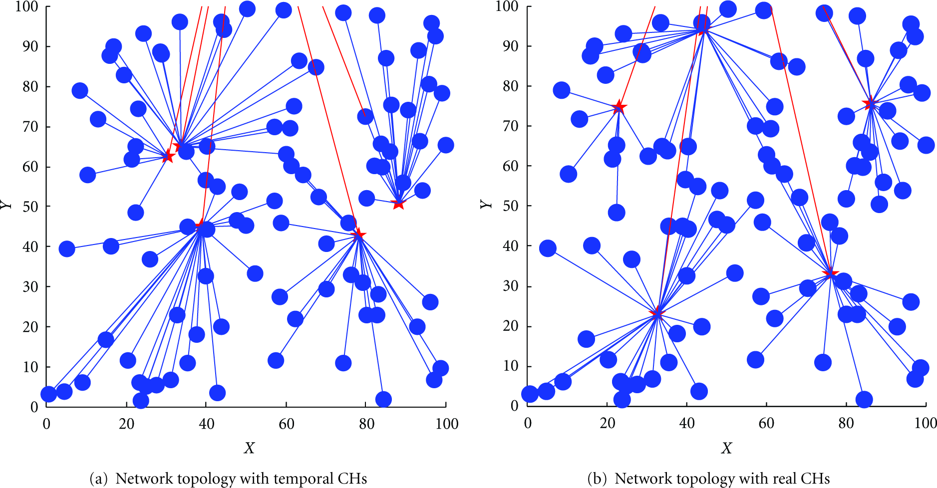
Topology transition under PARPEW.

The simulation analysis comprises four parts. First, we investigate the effect of two algorithmic parameters p (the probability of a node being a temporal CH) and α (the inequality aversion parameter). Second, we analyze the pattern generated by the number of sensors. Third, we illustrate the effect of base station location. Finally, we consider the case in which the initial energy level of the sensors is heterogeneous.

5.1. Experimental Setup

The experimental setup is similar to the one in [13] as summarized in Table 1. We randomly deployed 100 sensor nodes in a $100\hspace{0.17em}\hspace{0.17em}\times \hspace{0.17em}\hspace{0.17em}100$  m² two-dimensional square plane with the base station located at (50 m, 150 m). The WSN was used to monitor static situations, which means that every node sends a constant 5000 bits of data in every round. The comparative performance results of the three protocols are obtained using the same settings. The parameter values in Table 1 are basic values, some of which may be changed when testing the effect of different values. We replicated the simulation 100 times for each scenario to account for random variation.

Table 1

Basic simulation parameters used in the WSN.

Parameter	Value
Network size	$100\times 100$  m2
Number of sensor nodes	100
Initial energy	0.5 Joule
Location of the base station	(50 m, 150 m)
Data packet size	5000 bits
Control packet size	100 bits
Sensing radius	10 m
${\varepsilon }_{\text{elec}}$	50 nJ/bit
${\varepsilon }_{\text{tx}}$	50 nJ/bit
${\varepsilon }_{\text{rx}}$	50 nJ/bit
${\varepsilon }_{\text{amp}}$	100 pJ/bit/m2
${\varepsilon }_{\text{ag}}$	5 nJ/bit

5.2. Experimental Results

5.2.1. Effect of Algorithmic Parameters (p and α)

In this section, we investigate the effect of two PARPEW algorithmic parameters: p and α. As stated in Section 4, p represents the probability that a node will be a temporal CH (i.e., percentage of CHs) and α is the penalty for inequality. These two parameters significantly influence the performance of the protocol.

We evaluated the performance of protocols according to two definitions of lifetime: lifetime (99%) and Lifetime (95%), as shown in Figure 7(a). Because there were 100 sensor nodes, Lifetime (99%) was defined as the number of time period until the first sensor node dies. Similarly, Lifetime (95%) represents the amount of time until 5% of the nodes die. Figure 7(a) shows the lifetime of the different protocols ( $\alpha =2.2$ and $p=0.05$ in PARPEW). When PARPEW was used, Lifetime (99%) was approximately 340 rounds and Lifetime (95%) was approximately 360 rounds, which demonstrates gains of 42–47% over the LEACH and LEACH-C protocols. It is also evident that the PARPEW protocol outperforms the LEACH and LEACH-C protocols in all possible definitions of lifetime. Figure 7(b) plots the coverage over time, showing a pattern very similar to that of Figure 7(a).

Figure 7

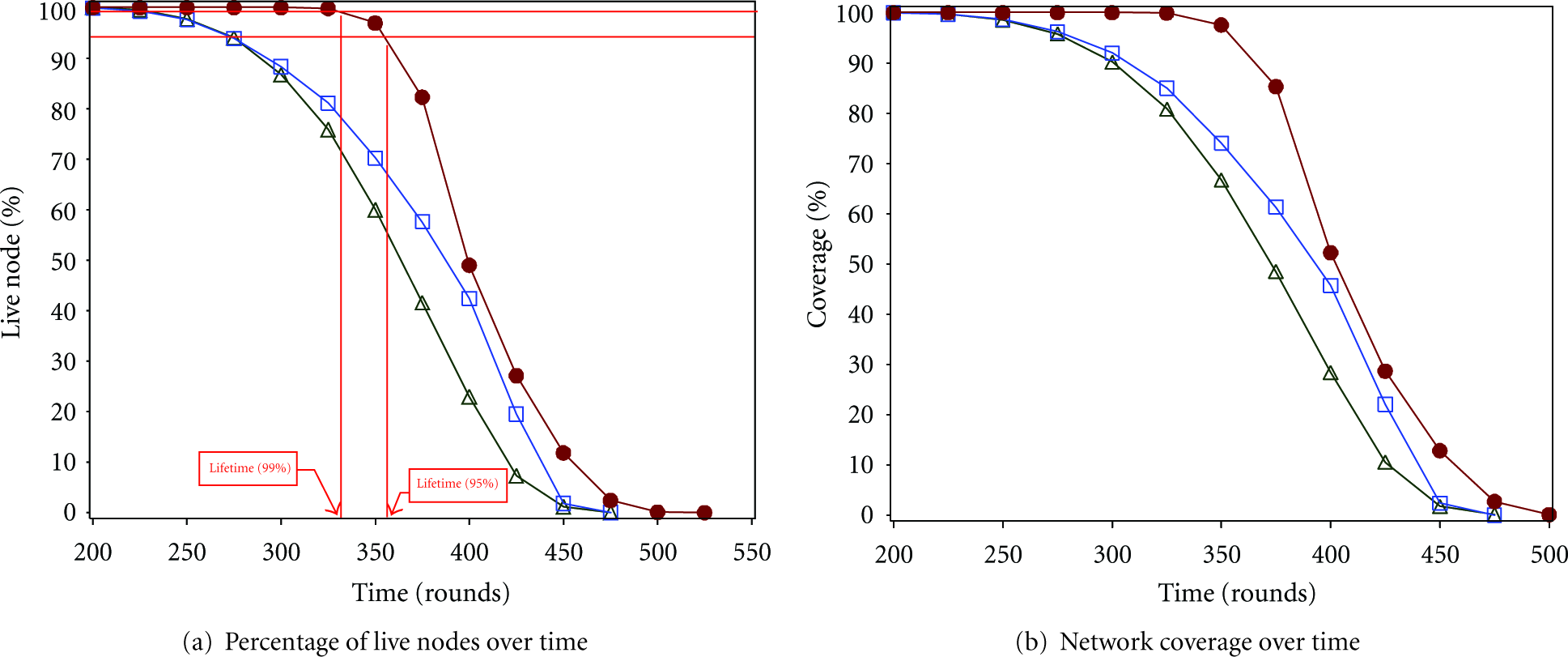
Percentage of live nodes and network coverage over time (rounds) with $\alpha =2.2$ and $p=0.05$ . Dark red circles represent results obtained from PARPEW. Open green triangles and blue squares represent simulation results from LEACH and LEACH-C, respectively (these representations are used in the following figures).

To analyze the effect of the two algorithmic parameters, we first vary α from 0.03 to 6.0 by fixing p at 0.05, because in [13], Heinzelman et al. proved that $p=0.05$ is optimal in the LEACH protocol. In Figure 8(a), the numerical results indicate that the best performance was achieved when α is 2.4. Lifetime (99%) does not significantly change after $\alpha =3.0$ . The result is also supported in the literature, where it is stated that it is useless to impose too much punishment to an inequality of a society.

Figure 8

Lifetime under various α and p values.

In the second step, we investigated the impact of the parameter p on Lifetime (99%). Figure 8(b) shows Lifetime (99%) values for both PARPEW and LEACH with the maximum lifetime occurring when p is between 0.05 and 0.08.

Figure 8(c) shows the effect of changing both α and p together, which significantly influenced the lifetime (statistically proven in two-way ANOVA analysis). The maximum lifetime occurred at $(\alpha ,p)=(\mathrm{2.4,0.05})$ , which are the values adopted for the remainder of this section.

5.2.2. Effect of the Number of Sensors

Figure 9 shows the effect of varying the number of sensors. Although the lifetime of the WSN increases as the number of sensors increases for any protocol, LEACH-C exhibits difficulty and poor scalability compared to the others. In addition, LEACH-C is a centralized protocol that is not scalable in computation and communication. Although the rate of improvement deteriorates as the number of sensors increases, the proposed PARPEW still achieves more than a 30% improvement over LEACH and LEACH-C.

Figure 9

Lifetime using various numbers of sensor nodes.

5.2.3. Effect of the Location of the Base Station

To analyze the impact of the location of the base station, we fixed the x-coordinate of the base station and varied the y-coordinate (designated as sink_Y in Figure 10), from 100 to 300 meters. It is clear that PARPEW performs well at short distances, prolonging the lifetime by up to 50%. Even when the distance is large, PARPEW still achieves an improvement of 12.5% and 37.8% over that of LEACH-C and LEACH, respectively. The results shown in Figure 10 indicate that the performance of the three protocols decreases as the distance to the base station increases. This occurs because increasing the distance to the base station implies an increase in transmission energy. The performances will be comparable above a certain Y value. That is because most of the energy will be spent on communication between the cluster heads and the base station. The energy savings from our protocol will be negligible compared to the huge communications cost.

Figure 10

Lifetime using various base station locations.

5.2.4. Effect of Heterogeneous Initial Energy Levels

We set the initial energy levels using normal distribution, $N(mean,{\mathit{\text{STD}}}^2)$ , set the mean at 0.5 Joules and varied STD from 0.05 to 0.15 Joules. In Figure 11, we can see that PARPEW performs better than LEACH and LEACH-C in all cases. The increase in the STD means that the initial energy levels of some sensors are very low, which accelerates the death of those sensor nodes. PARPEW prevents this by avoiding sensors with low energy residuals in the selection of CHs.

Figure 11

Lifetime using various initial energy distributions.

6. Conclusion

This paper introduces a novel cluster-based routing protocol for WSN to prolong the lifetime of WSNs. A WSN with a longer stable lifetime can be achieved when clusters are formed efficiently and data packets are redirected using EW as the decision metric to achieve both energy efficiency and energy balance throughout the network. The protocol, PARPEW, is implemented using an EW function that takes both residual energy and the distance matrix into consideration when computing the energy after transmission for predictive EW. Extensive experimental results demonstrate that when individual clusters in the WSN attempt to maximize their EW by switching CHs, global extension of the lifetime can be achieved.

The routing protocol can be extended in several ways. We assumed that a sensor node is capable of adjusting its transmission power without limitation. We plan to extend the protocol using a tree-based protocol to make it applicable in situations with limited transmission range. In addition, the application of alternative social welfare functions in addition to the one used in this research would also be valuable (e.g., Amartya, Sen, or Entropy).