Sage Journals: Discover world-class research

Abstract

In Alpine ski sport, traditional lap time measurement systems record a skier's departure and arrival using time-of-day timers through wires, which is not cost effective in unofficial or training games. This paper develops a lightweight lap time measurement system using a wireless sensor network, which employs a practical TDMA-based linear wireless sensor network protocol for multihop communications in long strap-shaped environments where sensor nodes are linearly deployed. We evaluate the performance of this protocol through the implementation and deployment of the lap time measurement system. The experimental results show that the proposed protocol transmits data at a success rate of 99.66% and maintains the time synchronization errors between two adjacent nodes within 183 μs without using any other time synchronization protocols. In an experimental deployment for a 1.5 km ski slope covered by 31 nodes, the system provides lap time measurements with a measurement error of 1.255 ms, which satisfies the official measurement error of 5.0 ms.

1. Introduction

Alpine ski sport was originated on Alps in Europe and so is named. In this sport, the rankings of ski racers are determined according to their lap times from a start line to a finish line. One distinctive feature of this sport is that skiers do not start at the same time, but at different times. International Ski Federation (FIS) recommends that the elapsed time of a skier skiing down a slope be recorded in a 10 ms unit with a timer synchronized to the time of day [1]. In traditional measurement systems, the departure signal at the start line and the arrival signal at the finish line are entered into an electronic stopwatch or a photo capture system through wires. These systems are not only expensive but also difficult to install for small-scale unofficial games. In this paper, we propose to develop a lightweight lap time measurement system based on a wireless sensor network (WSN) for Alpine ski sport, which employs a WSN protocol optimized in long-distanced outdoor surroundings such as ski slopes.

Many WSNs assume that sensor nodes are randomly distributed [2], as exemplified in Smart Dust [3]. In such networks, nodes near the destination send their own data and forward data from other nodes to a sink node by cooperating with neighbor nodes through designated RF channels. Studies based on the above concept of WSNs do not consider performance optimization in special cases where nodes are positioned in a particular way.

Among the first generation of WSNs, ALOHA [4] brought the simplicity of a 2-hop star topology shown in Figure 1(a) into its implementation. The current commercial WSNs such as wireless LAN [5], ZigBee [6], and bluetooth [7] adopt the simplest 1-hop star topology shown in Figure 1(b) as their basic function unit. Most existing research efforts, however, were focused on a general tree topology of WSNs shown in Figure 1(c). To the best of our knowledge, there exist very few studies that are tailored to the linear topology shown in Figure 1(d). Although a linear topology could be considered as a special case of a tree topology, a generic tree-based transport solution is unlikely to exploit the unique features of a linear topology for performance optimization.

Figure 1

Four types of node distributions in wireless sensor networks.

In fact, a significant number of practical applications feature a node distribution of type. (d) Examples of such linearly shaped WSN fields include monitoring systems for bridges, tunnels, borders, coastlines, fences, and ski slopes.

We propose a linear-wireless sensor network protocol, referred to as LSNP and design a lap time measurement system for Alpine ski sport based on LSNP. LSNP uses a TDMA MAC without the need of any time synchronization or routing protocols, and the measurement system is lightweight in terms of cost and operation. The performance of LSNP is evaluated through extensive experiments of the wireless lap time measurement system. Particularly, we implement the measurement system for a real-life deployment on a ski slope of about 1.5 km composed of three laps and covered with 31 nodes.

The rest of the paper is organized as follows. We describe some related work in Section 2 and propose LSNP in Section 3. The implementation and evaluation of LSNP and an LSNP-based lap time measurement system for Alpine ski sport are presented in Section 4 and Section 5, respectively. We conclude our work in Section 6.

2. Related Work

2.1. Wireless Lap Time Measurement System for Alpine Ski Sport

In FIS-defined wireless lap time measurement systems, the departure and arrival signals are entered into timers using wireless media instead of wires [1]. As such, FIS still adheres to a timer synchronized to the time of day. The proposed wireless measurement system, however, uses stable reference times generated by a linear-wireless sensor network protocol without any external timers.

2.2. Routing and Time Slot Assignment in TDMA MAC of WSN Protocols

In general, a routing layer separated from the MAC layer is needed in WSNs using CSMA MAC. MintRoute [8] is a routing protocol installed on TinyOS [9], where each node lets its neighbor nodes obtain required information to select their own parent node by broadcasting its routing information periodically in a network based on B-MAC [10] (a variant of CSMA MAC). As a result, MintRoute creates directed acyclic graph (DAG)-structured routing paths rooted on the sink node as a whole. The data routing paths from sensor nodes to the sink node can be established by combining assigned time slots in TDMA MAC.

DMAC [11] assigns the same time slot to all nodes of the same depth in a data gathering tree and lays out the time slots along the time line continuously as shown in Figure 2. The time slots of DMAC are allocated to overlap each other, that is, the sending period of the time slot for depth d overlaps with the receiving period of the time slot for depth $d - 1$ . This way, the sequence of time slots in DMAC acts as the role of a routing table towards the sink node. The nodes of the same depth in DMAC use a CSMA style MAC to avoid collisions and perform the node-to-node acknowledgement in the receiving period, resulting in a long overall transmission latency. Besides, DMAC does not specifically handle topology changes.

Figure 2

DMAC in a data-gathering tree.

FlexiTp [12], which is a variant of TDMA MAC, arranges nodes in a tree topology during the network setup phase and then assigns separate time slots to each node for transmitting its own data and forwarding the data from its child nodes. For example, in Figure 3, a series of time slots 6, 7, and 8 form a data transmission path from node D to the sink node S. In this case, a time slot assignment table also plays the role of a routing table in the network. However, this method suffers from reduced network bandwidth because it does not allow the sharing of overlapped routing paths, but assigns separate time slots to all routing paths.

Figure 3

An example of a routing path composed of time slots.

2.3. WSN Protocols for Linear Topology

Flush [13, 14] is designed to collect bulk data through a linear data gathering path in a tree-structured network between a source node and the sink node. Each node in flush forwards data packets captured from its next node with limited bandwidth. Node i of flush calculates its sending interval $d_{i} (= δ_{i} + H_{i - 1})$ with its own transmission time $δ_{i}$ and waiting time $H_{i - 1}$ to avoid interference with the transmission of its next nodes. As shown in Figure 4, since there are two nodes, that is, node $i - 2$ and node $i - 3$ , in the RF range of node $i - 1$ , $f_{i - 1} = δ_{i - 1} + δ_{i - 2}$ , and hence $d_{i} = δ_{i} + δ_{i - 1} + δ_{i - 2}$ , node i calculates $d_{i}$ by overhearing a packet of node $i - 1$ including $δ_{i - 1}$ and $f_{i - 1}$ , and this process is propagated one-by-one from node 1 to node n. Flush avoids collisions and reuses channels by ensuring that the bandwidth (sending interval) of node i does not exceed that of node $i - 1$ . The basic concept of flush considers time slots (not the assignment of time slots), and a CSMA MAC is used in the implementation of flush. Also, flush allows only one 1 : 1 data flow in the data gathering path, which is a severe restriction.

Figure 4

The concept of flush.

WiWi [15] is an improved WSN protocol of DMAC for linear topology. WiWi allows bidirectional communication by assigning downstream time slots and upstream time slots to each node one after the other as shown in Figure 5. WiWi avoids collisions by assuming that there are only two other nodes, that is, previous and next nodes, in the RF range of each node and does not allow network topology changes caused by node failures.

Figure 5

The concept of WiWi.

TSFP [16] is a pure TDMA WSN protocol improved from DMAC for linear topology where a new node joins the network as a terminal node one at a time, and there are no transmission collisions between nodes. The time slot of TSFP consists of three parts: receiving time, sending time, and acknowledging time. In Figure 6, node B processes acknowledgement by overhearing node A's packet including ACK for node B. The separation of acknowledging time in TSFP time slots improves the transmission latency performance of DMAC.

Figure 6

The concept of TSFP.

Although it has some merits as mentioned above, TSFP still suffers from critical performance limitations in networks deployed in a wide outdoor area. The first limitation of TSFP arises from the RSSI-based participation contention mechanism because RSSI is not strictly dependent on distance and is subject to momentary fluctuation, and therefore is no longer an appropriate index [14]. For example, as shown in Figure 7, TSFP forms a network of topology (b) if the RSSI value between nodes A–D is slightly better than that between nodes A-B. As a result, node T cannot join the network if the RSSI value between nodes B–T is unacceptably low. In this case, a network of topology (a) is more desirable in terms of the connectivity of the entire network even though the RSSI value between nodes A-B is lower than that between nodes A–D.

Figure 7

Issues in RSSI-based terminal join of TSFP.

The second limitation of TSFP restricts a new node to join the network as a terminal node only (we call it terminal join), which may result in some dangling nodes that are never able to join the network. For instance, in Figure 7(b), node T cannot join the network if node B and node T are outside of each other's RF range. Besides, the network has to be reorganized when new nodes must be added in the middle of the network as nonterminal nodes.

The third limitation is that, in case of a nonterminal node failure, all nodes that joined after the failed one become isolated from the network.

3. LSNP: Linear Wireless Sensor Network Protocol

We propose a practical linear wireless sensor network protocol, referred to as LSNP, which is improved from TSFP for a special type of WSNs deployed in long strap-shaped outdoor surroundings. To overcome the limitations of TSFP pointed out in Section 2, we incorporate into TSFP three new mechanisms to make it suitable for sensor networks with linear topology: address-based network participation process, nonterminal join process, and network recovery process.

3.1. Conceptual Model of LSNP

Structure of Time Slot Unit

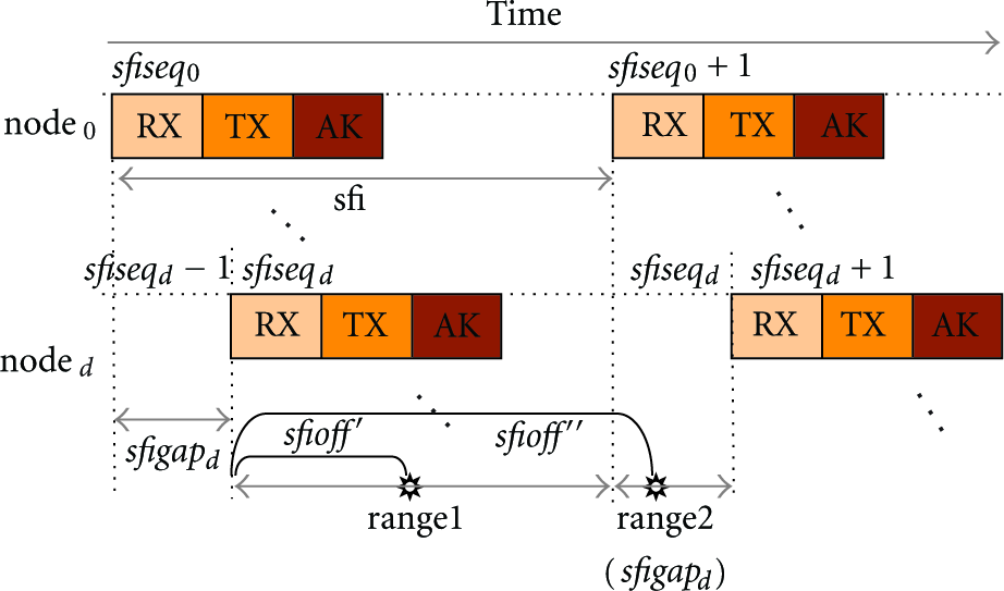
LSNP defines a time slot unit consisting of RF communication time and data processing time derived from RF transmission rate, MCU clock speed, and time synchronization error. As shown in Figure 8 each node has three consecutive time slot units (i.e., duty cycle time slots): reception (RX) slot, transmission (TX) slot, and acknowledgement (AK) slot. Each node's duty cycle time slot is repeated by a super frame interval period.

Figure 8

The concept of LSNP.

Allocation of Duty Cycle Time Slot

Most existing TDMA-based WSNs such as FlexiTP assign time slots to nodes [12]. In contrast, LSNP assigns nodes to time slots sequentially laid on the time line. Hence, in LSNP, the order of duty cycle time slots forms only one virtual link from the terminal node to the sink-node. The occupation of time slots in LSNP, namely, network participation of new nodes, is allowed by an existing node selected by the new node as shown in Figure 9.

Figure 9

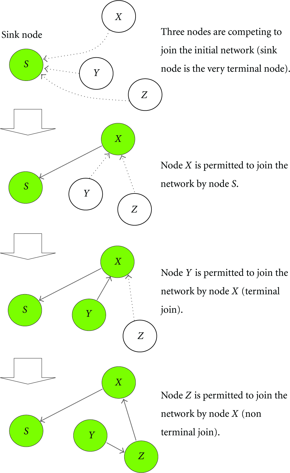
An example of the network growing phase of LSNP.

Time Synchronization

LSNP does not have a separate layer for time synchronization. As shown in Figure 10, $n o d e_{i}$ maintains its own frame reception time stamp $T r_{i}$ at the RX slot and frame transmission time stamp $T s_{i}$ at the TX slot by using a start of frame delimiter (SFD) interrupt, which is triggered at the time when a RF transceiver receives or transmits an SFD. $T r_{i - 1}$ is equal to $T s_{i}$ in global time if the RF propagation time and SFD interrupt latency are negligible. Hence, if $n o d e_{i - 1}$ inserts $T r_{i - 1}$ into the frame being transmitted to $n o d e_{i - 2}$ , $n o d e_{i}$ can obtain the global time offset between $n o d e_{i}$ and $n o d e_{i - 1}$ ( $= T s_{i} - T r_{i - 1}$ ) by overhearing the frame including $T r_{i - 1}$ at its AK slot. However, it is sufficient for TSFP to synchronize the clock of each node based on relative times between two adjacent nodes instead of the global time synchronization. It follows that $n o d e_{i}$ of TSFP achieves a time synchronization for its duty cycle time slot by initializing its timer with the remaining time until its next super frame interval based on $T r_{i}$ . This means that $n o d e_{i}$ is the basis of a time synchronization for $n o d e_{i - 1}$ , and time synchronization for the entire network is performed based on the clock of the terminal node.

Figure 10

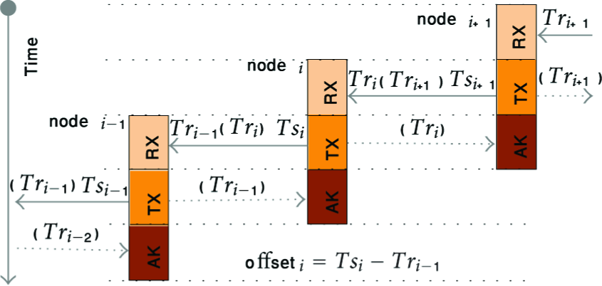
Time synchronization in LSNP.

Transmission of a Frame and an Acknowledgement

Each node builds the payload of a frame by aggregating data that have been forwarded node-by-node from the terminal node. Hence, the transmission of some data may be delayed until the next super frame interval because of the limit on the maximum size of the payload. In this case, it is possible to adopt various queue scheduling policies for quality of service (QoS) based on the priority of data. $N o d e_{i}$ verifies the acknowledgement for data transmission to $n o d e_{i - 1}$ by overhearing a frame transmitted by $n o d e_{i - 1}$ at its AK slot. If there is no acknowledgement, $n o d e_{i}$ does not remove the data from its queue, but attempts to retransmit them in the next super frame interval.

Routing

In LSNP, it is not necessary to create any separate routing layer since the order of duty cycle time slots itself forms a virtual link from the terminal node to the sink node.

3.2. Address-Based Network Organization

Instead of using the RSSI-based network self-organization, LSNP organizes a network based on node addresses, which are assigned to nodes in an ascending order from the sink node. Specifically, a new node that attempts to participate in an LSNP-based network first scans neighbor nodes in the network and then selects a node whose address is the nearest to and smaller than its own address as its parent node. For example, in Figure 11, new node N whose address is 11, selects node C whose address is 9, as its parent node. This way, LSNP builds an address-based linear network in an ascending order.

Figure 11

The address-based linear topology and nonterminal join in LSNP.

Obviously, the link quality of the entire network formed by LSNP is largely affected by low-quality links. The address-based network organization method of LSNP can avoid those node-to-node links with low link qualities by positioning the nodes at appropriate places.

3.3. Nonterminal Join

LSNP, which forms an address-based network, would need nonterminal join as shown in Figure 11 as well as the terminal join of TSFP. The nonterminal join process of LSNP is carried out in two phases: phase I (join-contention phase) and phase II (joining phase).

Phase I: Join-Contention Phase

(i)

New nodes scan their neighbor nodes and select their corresponding parent nodes based on the addresses of the scanned ones. They perform time synchronization with the selected parent nodes as shown in Figure 12 in the network active period of Figure 8 and then listen to the RF channel.

(ii)

A new node broadcasts JOIN_DCL (join-declaration message) at a join-contention time slot corresponding to its own address and carries out phase II.

(iii)

Other nodes wishing to join overhear JOIN_DCL, give up their attempts to join the network in the current super frame interval and try Phase I again in the next super frame interval. Obviously, low-numbered nodes (i.e., nodes that are close to the sink node) have high priority in the assignment of join-contention time slots.

Figure 12

The join-contention process of LSNP.

Phase II: Joining Phase

(i)

The new node that broadcasts JOIN_DCL at phase I synchronizes its own duty cycle time slot with the selected parent node's duty cycle time slot (step (a) in Figure 13).

(ii)

The new node overhears a frame that is forwarded to the parent node by the child of the parent node at the RX slot of the parent node and sends NTJN_REQ (nonterminal join request message) to the parent node immediately (step (b)).

(iii)

The parent node transmits a frame (step (c_1)) including SHFL_REQ (shift left one time slot unit request message) and NTJN_RES (nonterminal join response message) at its TX slot. On the other hand, the new node recognizes NTJN_RES by overhearing the frame (step (c_2)) at its TX slot.

(iv)

The new node and the parent node may be able to overhear the frame including SHFL_REQ transmitted to the grand parent node at their own AK slots (step (d_1) and (d_2)).

(v)

The parent node and other nodes positioned ahead of the parent node receive SHFL_REQ one by one and then advance their own duty cycle time slots exactly by a time period of one time slot unit (step (e)).

(vi)

If the new node fails to receive both of the messages (i.e., NTJN_RES in TX slot and SHFL_REQ in AK slot), it concludes that its NTJN_REQ has failed and then retries Phase I in the next super frame interval.

Figure 13

The nonterminal join process of LSNP.

3.4. Network Recovery

In LSNP, once a nonterminal node fails, the child node of that dead node sends a network recovery request message to its grand parent node to fill in the broken node's duty cycle time slot as shown in Figure 14. The detailed network recovery process of LSNP is described as follows (refer to Figure 15).

Figure 14

The network recovery concept of LSNP.

Figure 15

The network recovery process of LSNP.

(i)

The child node of a failed node sends RCVR_REQ (recovery request message) to the parent node of the dead node, that is, its grandparent node in its AK slot (step (a)).

(ii)

The grandparent node receives RCVR_REQ and transmits a frame including SHFR_REQ (shift right one time slot unit request message) and RCVR_RES (recovery response message) (step (b_1)).

(iii)

The child node is assured that RCVR_REQ has succeeded when it finds RCVR_RES at BK1 (blank 1) slot in the frame transmitted by its grandparent node (step (b_2)).

(iv)

The parent node and other nodes positioned ahead of the parent node in the network topology receive SFHR_REQ and back off their duty cycle time slot by a time period of one time slot unit.

(v)

If the child node fails to get the response to the network recovery request, it departs from the network, and then tries again with the first phase of the network participation process.

4. Implementation of LSNP and LSNP-Based Lap Time Measurement System for Alpine Ski Sport

4.1. Hardware and Software

4.1.1. Sensors for Detection of a Skier's Entry into a Lap of a Ski Slope

Sensors installed on the boundaries of laps detect the skier's entry into a lap (see the target deployment of the measurement system in Figure 19). There are a signal emitter on one side and a signal receiver on the other side as shown in Figure 16. An infrared or a laser sensor would be considered as a suitable sensing device for convenient installation in harsh outdoor environments with snowstorm and topographic irregularity in typical ski slopes. However, a laser sensor is more suitable than an infrared sensor because the latter may not be able to detect the skier's entry when she or he goes over a speed of 21 km/h. This is simply because the changed status of an infrared ray must be kept in receiver for a sufficiently long time in order to recognize the change. Note that the average speed of an Alpine skier is about 100 km/h.

Figure 16

Installation of laser sensors.

The laser sensor [17] used in this study is shown in Figure 17, and its specifications are provided in Table 1. An output terminal of the laser sensor receiver maintains 0 V while receiving the laser ray from the emitter and generates a 5 V pulse once the laser ray is shut off.

Table 1

Specification of laser sensors.

Items	Specifications
Model	LLS-1181L
Operating distance	50 m
Emitter	660 nm rot/rouge/red
Input	10–30 V DC
Output	5 V DC pulse
Switching frequency	6 KHz

Figure 17

Mote and laser sensor.

4.1.2. Sensor Node

The laser sensor output terminal is connected to a general purpose input/output (GPIO) pin of a sensor node equipped with an atmega 2560 8 bit micro controller unit (MCU) [18] whose specification is listed in Table 2. The GPIO pin is configured as a rising edge interrupt source. Figure 17 shows a snapshot of our mote for the implementation. A sensor node transmits a time stamp including the time when the interrupt occurs at the GPIO pin to the sink node through LSNP.

Table 2

Specification of sensor nodes.

Items		Specifications
MCU	Model	Atmega 2560 (7.3728 MHz, 30 PPM)
	Flash	256 KB
	RAM	8 KB
	Energy	active mode: 8 mA, sleep mode: 15 uA
External RAM		128 KB
RF transceiver		CC1100 ( $800 ~ 928$ MHz, 500 kbps max)
Antenna type		1/4 λ mono pole
Power source		2 AA type lithium batteries (3.6 V)

4.1.3. Coding of LSNP

As shown in Figure 18, the frame of LSNP contains the following fields: frame length, frame header, and optional protocol data units (PDU) that carry sensing data. Each PDU in the frame is prioritized and is composed of PDU id, the PDU length, and the corresponding information. Upon the receival of a frame, LSNP parses its contents and inserts the PDUs into the local queues if they are not destined to itself. The PDUs including those of its own in the queues are reassembled into a frame before transmission. In case of frame overflows, the PDU's priority is taken into consideration to determine which PDUs should be sent first. LSNP is implemented using WinAVR gcc compiler [19] in AVR studio 4.18 [20] and it runs without any operating systems. Its code and data sizes are about 48 KB and 4 KB, respectively.

Figure 18

Format of the LSNP frame.

Figure 19

A target deployment environment of the lap time measurement system.

4.2. Configuration of LSNP in a Target Deployment Environment

4.2.1. A Target Deployment Environment

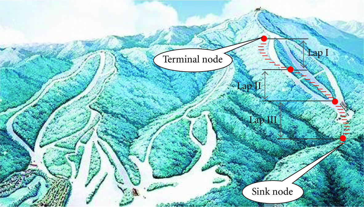
The LSNP-based lap time measurement system is to be deployed on a ski slope as shown in Figure 19. We place 31 nodes (excluding the sink-node) with a span of about 50 m to cover the ski slope of about 1,500 m. Since the maximum available communication range in the ski slope is about 150 m when the output power of RF transceiver CC1100 [21] in Table 2 is about 7 dBm, the 50 m span placement makes it possible for LSNP to maintain the network connected by the network recovery process even if two consecutive node fail to function.

The node addresses are numbered in an ascending order from 0 (sink-node) to 31. Four nodes that are capable of detecting a skier's passing by a laser sensor are located at the starting point (the terminal node with node address 31), 500 m point (node address 21), 1,000 m point (node address 11), and finish line (node address 1). All other nodes are relay nodes that relay the time measurements to the sink node.

4.2.2. Configuration of LSNP

In this subsection, we provide the details on the configuration of LSNP: super frame interval, RF transmission rate, frame size, interrupt and data processing time, time errors caused by XTAL (crystal) vibration error, and resolution of MCU timer counter.

Frame Transmission Time

We use 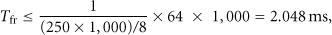$T_{fr}$ to denote the time for a node to transmit a frame completely. The transmission rate and maximum frame size of RF transceiver CC1100 are configured as 250 kbps (maximum baud rate) and 64 bytes (same as RX/TX FIFO buffer size), respectively. Then, we have the following inequality for $T_{fr}$ :

T_{fr} \leq \frac{1}{(250 \times 1,000) / 8} \times 64 \times 1, 000 = 2.048 ms,

(1)

where (250 × 1,000)/8 is the number of bytes transmitted per second, and 1/((250 × 1,000)/8) is a time period, in second, to transmit 1 byte.

Data Processing Time

We use $T_{dp}$ to denote the time for a node to process data after a frame is received or before a frame is sent. The clock speed of atmega 2560 MCU in Table 2 is 7.3728 MHz, while the average instruction execution time is less than 2 cycles. Also, the number of instructions for data processing is less than 12,000 steps. Therefore, we have the following inequality for $T_{dp}$ :

T_{dp} \leq \frac{1}{7, 372, 800} \times 2 \times 12, 000 \times 1, 000 < 3.256 ms .

(2)

SFD Interrupt Latency and Handling Time

We use $T_{sfd}$ to denote SFD interrupt latency and handling time. Interrupt latency is the time elapsed in context switching. We observed that SFD interrupt latency is about 16 μs, and the number of instructions in the SFD interrupt handling routine of the system is less than 1,500 steps. Therefore, we have the following inequlity for $T_{sfd}$ :

\begin{matrix} T_{sfd} & \leq 0.016 + (\frac{1}{7, 372, 800} \times 2 \times 1, 500 \times 1, 000) \\ < 0.423 ms . \end{matrix}

(3)

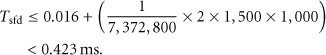
Time Error Caused by Resolution of Timer Counter

We use $E_{tmo}$ to denote the maximum time error that is caused by the resolution of timers between two adjacent nodes. A timer of 0.9216 MHz prescaled by eight from one of the six timers of Atmega 2560 MCU is used for time synchronization in the system. The original clock source of the timer is the MCU clock of 7.3728 MHz. A value of the timer counter is usually represented in unit of tic. Hence, 1 tic represents one increment in the timer counter of 0.9216 MHz in the system. Accordingly, we define $E_{tmo}$ as follows:

E_{tmo} = 2 tics = \frac{1}{921, 600} \times 2 \times 1,000 ms < 0.003 ms .

(4)

Time Error Caused by XTAL Vibration Error

We use $E_{xtl}$ to denote the maximum time error that is caused by the XTAL vibration error between two adjacent nodes in a single super frame interval. The precision of XTAL used for atmega 2560 MCU in our sensor node platform is 30 PPM, which means that the maximum vibration time error of the XTL is 30 μs per second compared with the absolute real time. Since the value of super frame interval is set to 3 seconds (the value of super frame interval will be explained later in this subsection), $E_{xtl}$ is calculated as follows:

E_{xtl} = 0.00003 \times 3 \times 2 \times 1, 000 = 0.18 ms .

(5)

Configuration of Time Slot Unit

We use $T_{unit}$ to denote the length of a time slot unit. We configure $T_{unit}$ as shown in Figure 20 by taking into account various time factors described above. We use the unit of tic for $T_{unit}$ for convenience in managing the timer counters. $T_{guard}$ in Figure 20 is a guard time that includes the following three time factors: (i)

0.18 ms for the maximum time error caused by the timer counter resolution and XTAL vibration error between two adjacent nodes in a super frame interval ( $E_{tmo} + E_{xtl}$ );

(ii)

0.5 ms for the power on/off time of the RF transceiver;

(iii)

1.0 ms for the output time of a 10 bytes long debugging message through UART (Universal Asynchronous Receiver/Transmitter) device with 11.52 kbps.

Figure 20

A time slot unit of the LSNP-based lap time measurement system.

Configuration of Super Frame Interval

We use $T_{sfi}$ to denote the super frame interval for which a node's duty cycle time slot is repeated periodically. $T_{sfi}$ determines the maximum transmission delay for a node to wait before it sends measurement data (time stamps) to the sink node. As shown in Figure 8, $T_{sfi}$ is defined as follows:

T_{sfi} = network active period + network inactive period .

(6)

Clearly, the network active period is defined as the number of nodes in the network times $T_{unit}$ plus double of $T_{unit}$ , and the range of its value in the system is given as follows:

\begin{matrix} 348.632 ms & < network active period = (32 + 2) \times T_{unit} \\ = 321,300 tics < 348.633 ms . \end{matrix}

(7)

It is also necessary to reserve a time period for join-contention time slots in the network inactive period, and it is reasonable to configure the join-contention time slot as

T_{fr}

. Due to the assignment of a separate join-contention time slot to each node, the network inactive period should be greater than or equal to the value of

T_{fr}

times the number of nodes in the network except the sink node. Therefore, the following inequality holds:

\begin{matrix} 31 \times 2, 250 tics & = 69,750 tics < 75.684 ms \\ \leq network inactive period . \end{matrix}

(8)

From (7) and (8), the minimum value of

T_{sfi}

in our system is about 409.203 ms, namely:

\begin{matrix} T_{sfi} & = network active period + network inactive period \\ > 348.633 ms + 75.648 ms . \end{matrix}

(9)

The time synchronization accuracy, the node energy consumption, and the transmission delay of the proposed system are affected directly by

T_{sfi}

. Apparently, the shorter the super frame interval is, the more accurate the time synchronization is; on the other hand, the longer the super frame interval is, the less energy consumption the system has. The average transmission delay is about

T_{sfi}

/2. Under all possible circumstances, 1 or 2 seconds would be appropriate for

T_{sfi}

. We, however, set

T_{sfi}

to be 3 seconds in order to tolerate harsher conditions for time synchronization as the accuracy of the lap time measurement of the proposed system is of the highest interest to us.

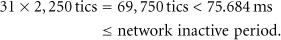
Activities of Each Node

Each node changes the RF state to the receiving mode, listens to the RF channel at the start time of $T_{guard 1}$ of the RX and AK slots, and waits for a frame's arrival until the end time of $T_{guard 2}$ . At the start time of $T_{guard 1}$ of TX slot, each node changes the state of RF transceiver to the transmission mode and starts to transmit a frame at the start time of $T_{sfd}$ .

4.3. Time Stamp

Upon the receival of an interrupt signal triggered by a laser sensor, the sensor node generates a time stamp and then sends it to the sink node at its TX slot in a node-by-node manner. The sink node sends the time stamp to a remote server system via a gateway that is connected through wire to the sink node. Laser sensor interrupts may be triggered at any time along the time line as shown in Figure 8. Each sensor node generates a relative time stamp based on its own super frame interval. The relative time stamp is converted to an absolute time stamp to be used for record estimation in a server system. In this paper, all of the time information is measured in unit of tic of 0.9216 MHz timer. The relationship between the tic unit time $T_{tic}$ and the ms unit time $T_{ms}$ is defined as

T_{ms} = T_{tic} \times \frac{(1 / 921,600)}{1,000} .

(10)

Realtive Time Stamp (Node Time Stamp)

Each sensor node constructs a time stamp consisting of three components, that is, super frame interval sequence (sfiseq), time past in the super frame interval (sfioff), and its own depth (d). The sfiseq of each node is increased by one at the start time of duty cycle time slot of the node. Meanwhile, depth d of each node is set to be one plus the depth value that is included in the frame transmitted by its child node, as shown in Figure 21. The depth d does not change if there is no change in the network's topology. Note that the depth of the terminal node is always 0.

Figure 21

Relative time stamp of $n o d e_{d}$ with depth d.

Absolute Time Stamp (Server Time Stamp)

The relative time stamps of the sensor nodes collected in a server system are converted to absolute time stamps based on the super frame interval of the terminal node. The relative time stamp of $n o d e_{d}$ whose depth is d, as shown in Figure 21, is converted into an absolute time stamp using the procedure provided in Algorithm 1. In Figure 21, sfigap represents the time difference between the start times of duty cycle time slot of $n o d e_{0}$ and $n o d e_{d}$ . The relative sfiseqs of $n o d e_{d}$ and $n o d e_{0}$ are the same if the relative sfioff of $n o d e_{d}$ lies in range1, while the relative sfiseq of $n o d e_{0}$ is one step ahead in the case where the relative sfioff of $n o d e_{d}$ lies in range2.

Algorithm 1: Procedure of translating relative time stamp to absolute time stamp of $n o d e_{d}$ .

sfigap_d = d × time_slot_unit; /* depth d*/

if (sigoff_d < (sfi − sfigap_d ) /* sfioff’ of range1*/

sfioff_d = sfigap_d + sfioff_d;

else { /* sfioff” of range2*/

sfiseq_d = sfiseq_d + 1;

sfioff_d = sfigap_d − (sfi − sfioff_d);

}

Calculation of a Lap Time

We use 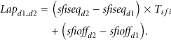$L a p_{d 1_d 2}$ to denote the lap time between two sensor nodes whose depth is $d 1$ , $d 2$ ( $d 1 < d 2$ ), respectively. $L a p_{d 1_d 2}$ is calculated from the absolute time stamps converted from the relative time stamps as follows:

\begin{matrix} L a p_{d 1_d 2} & = (s f i s e q_{d 2} - s f i s e q_{d 1}) \times T_{s f i} \\ + ({s f i o f f}_{d 2} - s f i o f f_{d 1}) . \end{matrix}

(11)

5. Evaluation of the LSNP-Based Lap Time Measurement System

5.1. Functionality of LSNP

For testing purposes, we deployed the sensor nodes for the ski slope in Figure 19 on the campus of Gangneung-Wonju National University as shown in Figure 22. Each node was packed in a plastic case and tied to the pole of a street lamp at 2 m high from the ground. The total length of the linear network formed by LSNP is about 1.2 km. The average span distance between two street lamp poles is about 40 m. Four sensor nodes ( $n o d e_{31}$ , $n o d e_{21}$ , $n o d e_{11}$ , and $n o d e_{1}$ ), which are responsible for detecting a skier's passing, were configured to generate pseudo time stamps every 100 super frame intervals (about 5 minutes) for 3 weeks (604,800 super frame intervals). Table 3 lists the experimental results, which shows that LSNP achieves a reasonably high data transmission success rate when deployed in an outdoor environment. The transmission success rate of higher than 99% in the functionality test demonstrates that LSNP is sufficiently reliable to transmit the lap time measurement data wirelessly in an Alpine ski game environment.

Table 3

The success rate of LSNP data transmission.

Sensor node	Number of expected time stamps	Number of collected time stamps	Rate of success (%)
Node₁	6,048	6,042	99.90
Node₁₁	6,048	6,030	99.70
Node₂₁	6,048	6,021	99.55
Node₃₁	6,048	6,016	99.47

Total	24,192	24,109	99.66

Figure 22

Deployment of nodes in a test network environment.

5.2. Theoretical Maximum Time Synchronization Error between Multihop Nodes

We use $E L_{n}$ to denote the theoretical maximum time synchronization error between the first node and the last one in a lap of n hops in a super frame interval ( $T_{s f i}$ ). We define $E L_{n}$ as follows based on (4) and (5):

E L_{n} = (E_{tmo} + E_{xtl}) \times n < 0.183 n ms .

(12)

Equation (12) shows that the maximum time synchronization error between two adjacent nodes in a super frame interval, namely,

E L_{1}

is less than 0.183 ms. All maximum time synchronization errors of lap I, lap II, and lap III are

E L_{10}

since those laps are all covered by 11 nodes according to the node deployment in Figure 19. Therefore,

E L_{10}

is less than 1.83 ms, and the maximum time synchronization error of the entire slope covered by 31 nodes, namely,

E L_{30}

, is less than 5.49 ms. The theoretical maximum time synchronization error is slightly greater than 5 ms, which is the requirement for the ski sport record measurement [1].

5.3. Actual Time Synchronization Error between Multihop Nodes

To evaluate the actual time synchronization errors between multihop nodes, we deployed the nodes on an office floor as shown in Figure 23 and connected the extensions of the laser sensor output cables (see Table 1) to the oscilloscope channels in order to measure the absolute real-time synchronization and measurement errors of the LSNP-based lap time measurement system. We would like to point out that we used the same oscilloscope as used in the conventional wired system because the oscilloscope is one of the most precise real-time stop watches recommended by International Ski Federation (FIS). The high precision of this device makes the measuring process of our wireless system comparable with that of the wired system. The only factor that may affect the time synchronization errors between the indoor test and the outdoor test is the temperature of crystal equipped in the nodes (see (5)). To investigate the impact of the crystal temperature, we stored several nodes in a refrigerator of −15°C and compared their clock speed with that of the nodes outside of the refrigerator. We did not observe any distinguishable differences between these two groups of sensors.

Figure 23

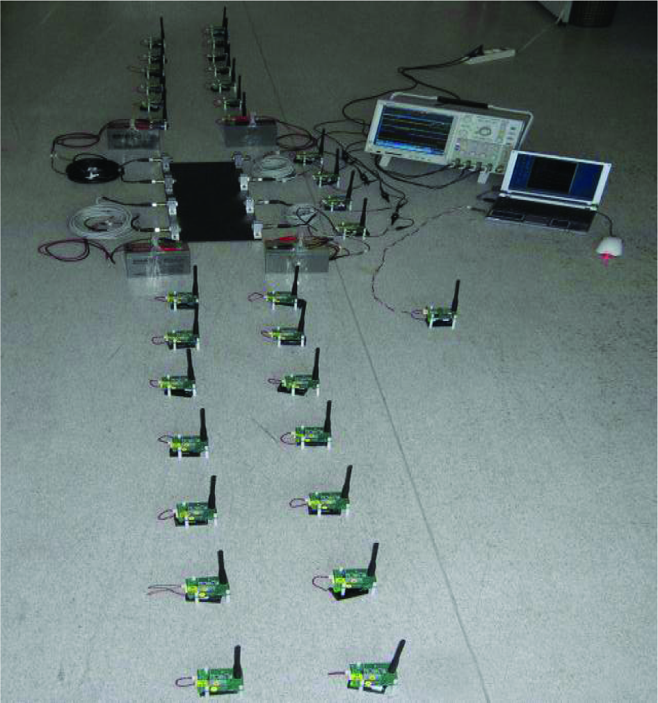
Deployment of nodes for testing time synchronization errors of LSNP.

To produce test data, we shut the laser beams off manually with a colored plastic ruler. The laser sensor produces a 5 V DC pulse immediately when the laser beam is shut off. The pulse interrupts the sensor node and at the same time generates a trigger at the oscilloscope. We performed the experiment 100 times every 5~10 minutes for 12 hours in both 1-hop and 10-hop environments.

5.3.1. Actual Time Synchronization Error between Two Adjacent Nodes (Laps of 1-Hop Length)

The time synchronization error between two adjacent nodes in the proposed measurement system may be obtained by comparing their time stamps that are generated in response to a single interrupt source. In this test, we select a laser sensor and connect its output terminal to the four sensor nodes ( $n o d e_{31}$ , $n o d e_{21}$ , $n o d e_{11}$ , and $n o d e_{1}$ ) in parallel. By only turning on the power of the four sensor nodes, we get three laps of 1-hop length, that is, the laps of $n o d e_{31}$ - $n o d e_{21}$ , $n o d e_{21}$ - $n o d e_{11}$ , and $n o d e_{11}$ - $n o d e_{1}$ . Table 4 shows the time synchronization errors between adjacent nodes that were calculated from the 100 experiments above. Table 4 shows that the actual time synchronization errors between two adjacent nodes did not exceed $E L_{1}$ ( $= 0.183 ms \approx 169 tics$ ).

Table 4

Actual time synchronization errors between two adjacent nodes, (unit: 0.9216 MHz tic (ms)).

Metrics	1-hop lap
Metrics	node₃₁-node₂₁	node₂₁-node₁₁	node₁₁-node₁

Average	0.1 (0.000)	27.0 (0.003)	32.9 (0.004)
Standard deviation	3.9 (0.000)	16.5 (0.002)	14.6 (0.002)
Max.	19.0 (0.002)	44.0 (0.005)	108.0 (0.012)
Min.	−31.0 (0.004)	−16.0 (0.002)	−21.0 (0.003)
Max deviation	50.0 (0.005)	60.0 (0.007)	129.0 (0.014)

5.3.2. Actual Time Synchronization Error in Laps of 10-Hop Length

If all of the relay nodes are powered up in the above experimental environment, the four sensor nodes build up three laps of 10-hop length, that is, the laps of $n o d e_{31}$ - $n o d e_{21}$ , $n o d e_{21}$ - $n o d e_{11}$ , and $n o d e_{11}$ - $n o d e_{1}$ . Table 5 shows the results of the actual time synchronization errors when the experiment is carried out in the same way as that of Table 4. Table 5 shows that the actual time synchronization errors of laps of 10-hop length are sufficiently smaller than $E L_{10}$ ( $= 1.83 ms \approx 1690 tics$ ).

Table 5

Actual time synchronization errors of laps of 10-hop length, (unit: 0.9216 MHz tic (ms)).

Metrics	10-hop lap
Metrics	node₃₁-node₂₁	node₂₁-node₁₁	node₁₁-node₁

Average	0.7 (0.000)	149.0 (0.017)	244.8 (0.027)
Standard deviation	44.4 (0.049)	86.3 (0.010)	121.6 (0.014)
Max.	99.0 (0.011)	288.0 (0.033)	482.0 (0.053)
Min.	−140.0 (0.016)	−141.0 (0.016)	−104.0 (0.012)
Max deviation	239.0 (0.026)	429.0 (0.047)	590.0 (0.064)

5.3.3. Some Trends in the Actual Time Synchronization Errors

Tables 4 and 5 indicate that the entire distribution of the time synchronization errors is biased towards positive values. This implies that it is possible to reduce the deviation of the errors by tuning the results.

Figure 24 shows curves of the theoretical and actual time synchronization errors depending on the number of hops. The experimental results were obtained for 1-hop, 2-hop, 3-hop, 10-hop, 20-hop, and 30-hop in the same experimental environment as those of Tables 4 and 5. Figure 24 shows that the longer the lap length is, the larger the error margin in the realization of time synchronization is. In other words, the gap between the actual time synchronization error and the corresponding maximum time synchronization error increases as the lap becomes longer. For example, the error margin of lap $n o d e_{31}$ - $n o d e_{1}$ covered by 31 nodes is $3,948$ ( $5,070 - 1,122$ ) tics while that of lap $n o d e_{11}$ - $n o d e_{1}$ covered by 11 nodes is $1,104$ ( $1,690 - 586$ ) tics. This observation implies that there is a room to mitigate the increase in the maximum time synchronization errors of LSNP as the number of nodes increases. Another noticeable observation is that even if the lengths of two laps are equal, the farther a lap is located away from the terminal node, the larger its time synchronization error is. For example, the time synchronization error of 239 tics for the 10-hop lap $n o d e_{11}$ - $n o d e_{1}$ is smaller than 586 tics for the 10-hop lap $n o d e_{31}$ - $n o d e_{21}$ . These two features of the actual time synchronization errors in Figure 24 could be utilized in calibrating the proposed lap time measurement system.

Figure 24

Trends of actual time synchronization errors.

5.4. Measurement Error of Lap Times

We measured the lap times by connecting the outputs of the laser sensors to the four sensor nodes ( $n o d e_{31}$ , $n o d e_{21}$ , $n o d e_{11}$ , $n o d e_{1}$ ) and using all of the relay nodes in Figure 23. Four outputs of the laser sensors are connected to four channels of the oscilloscope to measure the lap times in a highly accurate way in terms of absolute time. In the experimental configuration, we evaluate the performance of the LSNP-based lap time measurement system with reference to real-time signals on the oscilloscope console. To generate test data for comparison, we passed through each lap with an interval of about 20 seconds, which is roughly similar to the actual records in Alpine skiing games. This experiment was done 100 times in an interval of 7 to 13 minutes, spanning 16 hours or so.

Table 6 shows the experimental results. The measurement system was precalibrated based on the previous results before the experiment. Table 6 justifies that the proposed measurement system can measure lap times in an error range of 1.255 ms even in the case where the length of a lap is less than or equal to 30 hops.

Table 6

Experimental lap time measurement errors, (unit: ms).

Metrics	1-hop lap
Metrics	node₃₁-node₂₁ (10-hop)	node₂₁-node₁₁ (10-hop)	node₁₁-node₁ (10-hop)	node₃₁-node₁₁ (20-hop)	node₂₁-node₁ (20-hop)	node₃₁-node₁ (30-hop)

Average	−0.001	0.001	0.001	0.001	0.001	−0.001
Standard deviation	0.194	0.183	0.187	0.188	0.182	0.214
Max.	0.345	0.424	0.527	0.387	0.724	0.412
Min.	−0.532	−0.507	−0.586	−0.566	−0.531	−0.615
Max deviation	0.877	0.931	1.113	0.953	1.255	1.026

5.5. Field Test of the Lap Time Measurement System

To test the lap time measurement system in a real ski environment, we deployed the system on the Rainbow III ski slope as shown in Figure 19, which is the second longest international ski slople in YongPyong Ski Resort located in Daegwallyeong-myeon, Pyeongchang, Gangwon-do, South Korea. Table 7 lists the deployment environment conditions of the ski slope. Yongpyong was a candidate resort for the 2010 and 2014 winter olympics and is to hold the 2018 winter olympics. This resort has several ski slopes certified by the FIS and has hosted races in both the alpine and disabled alpine world cups.

Table 7

Environmental conditions for field test.

Items		Values
Start line	Altitude	1,458 m
Start line	Temperature	−2°C (windy)

	Length	1,520 m
	Height (drop)	500 m
Slope	Highest tilt	49°
	Average tilt	36°
	Lowest tilt	15°

Finish line	Temperature	6°C (cloudy)

We packed each sensor node in a small plastic case and tied it to the top of a thin iron pole of about 1 m as shown in Figure 25. In our test, six skiers skied the slope one at a time in an interval of 25 minutes, and the system continuously collected the lap time measurements. Throughout the test, the system operated smoothly and the measurement results confirm our previous performance analysis.

Figure 25

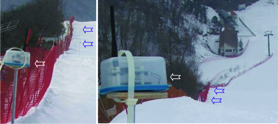
Installation of nodes for the field test.

6. Conclusion

We proposed a practical TDMA-based WSN protocol named LSNP that is dedicated to a class of sensor network application fields where nodes are placed in a linear fashion in a long strap-shaped environment. Based on LSNP, we implemented a lap time measurement system specialized for Alpine skiing games and demonstrated the efficacy of LSNP by evaluating the performance of the proposed measurement system in various experiments. The experimental results showed that the data transmission success rate of LSNP was about 99.66% and LSNP was capable of measuring the lap times with a measurement error of less than 1.255 ms without any additional time synchronization protocol in a network of 32 nodes. The results also satisfied the theoretical maximum time synchronization error of 183 μs between two adjacent nodes and met the requirement of 5 ms in official skiing lap time measurement systems. The proposed LSNP-based lap time measurement system is proved to be useful for training skiers or measuring unofficial lap times in Alpine ski games.

The lap time measurement system is one representative application of the proposed LSNP approach, which has great potential of being used in many other applications deployed in long-distanced outdoor surroundings such as bridges, tunnels, borders, coastlines, and fences.

References

FIS (International Ski Federation) TIMING-BOOKLET, Version 2.45, October 2010, http://www.fis-ski.com/data/document/timingbooklet-v2_45.pdf

Akyildiz

I. F.

Sankarasubramaniam

Cayirci

Wireless sensor networks: a survey

Computer Networks 2002 38 4 393 422

2-s2.0-0037086890

10.1016/S1389-1286(01)00302-4

Warneke

Last

Liebowitz

Pister

K. S. J.

Smart dust: communicating with a cubic-millimeter computer

Computer 2001 34 1 44 51

2-s2.0-0035121216

Abramson

THE ALOHA SYSTEM-another alternative for computer communications

Proceedings of the American Federation of Information Processing Societies Joint Computer Conferences (AFIPS '70)

1970

New York, NY, USA

281 285

IEEE Computer Society Wireless LAN Medium Access Control (MAC) and Physical Layer (PHY) Specifications (ANSI/IEEE Std. 802.11-2007), 2007

ZigBee Alliance ZigBee Specification, Document 053474r17, 2008

Bluetooth SIG Specification of the Bluetooth System Core, Version 1.2, 2003

Woo

Tong

Culler

Taming the underlying challenges of reliable multihop routing in sensor networks

Proceedings of the 1st International Conference on Embedded Networked Sensor Systems (SenSys '03)

November 2003

14 27

Hill

Szewczyk

Woo

Hollar

Culler

Pister

System architecture directions for networked sensors

Proceedings of the 9th Internatinal Conference on Architectural Support for Programming Languages and Operating Systems (ASPLOS '00)

November 2000

93 104

10.

Polastre

Hill

Culler

Versatile low power media access for wireless sensor networks

Proceedings of the 1st International Conference on Embedded Networked Sensor Systems (SenSys '04)

November 2004

95 107

11.

Krishnamachari

Raghavendra

C. S.

An adaptive energy-efficient and low-latency MAC for data gathering in wireless sensor networks

Proceedings of the 18th International Parallel and Distributed Processing Symposium (IPDPS '04)

April 2004

3091 3098

12.

Lee

W. L.

Datta

Cardell-Oliver

FlexiTP: a flexible-schedule-based TDMA protocol for fault-tolerant and energy-efficient wireless sensor networks

IEEE Transactions on Parallel and Distributed Systems 2008 19 6 851 864

2-s2.0-44049089919

10.1109/TPDS.2007.70774

13.

Kim

Fonseca

Tavakoil

Flush: a reliable bulk transport protocol for multihop wireless networks

Proceedings of the 1st International Conference on Embedded Networked Sensor Systems (SenSys '07)

2007

New York, NY, USA

351 365

14.

Pakzad

S. N.

Fenves

G. L.

Kim

Culler

D. E.

Design and implementation of scalable wireless sensor network for structural monitoring

Journal of Infrastructure Systems 2008 14 1 89 101

2-s2.0-39549092827

10.1061/(ASCE)1076-0342(2008)14:1(89)

15.

Caneva

D. D.

Montessoro

P. L.

A synchronous and deterministic MAC protocol for wireless communications on linear topologies

International Journal of Communications, Network and System Sciences 2010 3 12 925 933

16.

Kim

D. S.

Lee

S. Y.

Won

K. H.

Chung

D. J.

Kim

J. H.

Time-synchronized forwarding protocol for remote control of home appliances based on wireless sensor network

IEEE Transactions on Consumer Electronics 2007 53 4 1427 1433

2-s2.0-39549095645

10.1109/TCE.2007.4429233

17.

CTX Korea Inc. 2009, http://www.contrinex.co.kr/product/pdf/low.pdf

18.

Atmel Corporation 8-bit AVR Micro controller with 64K/128K/256K Bytes In-system Programmable Flash (Data Sheet Rev. M), 2010, http://www.atmel.com/dyn/resources/prod_documents/doc2549.pdf

19.

Weddington

E. B.

WinAVR User Manual, 2010, http://dybkowski.net/download/winavr-user-manual.html

20.

Atmel Corporation AVR Studio 4.18, 2009, http://www.atmel.com/dyn/products/tools_card.asp?tool_id=2725&category_id=163&family_id=607&subfamily_id=760

21.

Texas Instruments Corporation CC1100 Low-Power Sub-1GHz RF Transceiver (Data Sheet Rev. D), 2009, http://www.ti.com/general/docs/lit/getliterature.tsp?genericPartNumber=cc1100&fileType=pdf

A Lightweight Lap Time Measurement System for Alpine Ski Sport Using a TDMA-Based Linear Wireless Sensor Network

Abstract

1. Introduction

2. Related Work

2.1. Wireless Lap Time Measurement System for Alpine Ski Sport

2.2. Routing and Time Slot Assignment in TDMA MAC of WSN Protocols

2.3. WSN Protocols for Linear Topology

3. LSNP: Linear Wireless Sensor Network Protocol

3.1. Conceptual Model of LSNP

Structure of Time Slot Unit

Allocation of Duty Cycle Time Slot

Time Synchronization

Transmission of a Frame and an Acknowledgement

Routing

3.2. Address-Based Network Organization

3.3. Nonterminal Join

Phase I: Join-Contention Phase

Phase II: Joining Phase

3.4. Network Recovery

4. Implementation of LSNP and LSNP-Based Lap Time Measurement System for Alpine Ski Sport

4.1. Hardware and Software

4.1.1. Sensors for Detection of a Skier's Entry into a Lap of a Ski Slope

4.1.2. Sensor Node

4.1.3. Coding of LSNP

4.2. Configuration of LSNP in a Target Deployment Environment

4.2.1. A Target Deployment Environment

4.2.2. Configuration of LSNP

Frame Transmission Time

Data Processing Time

SFD Interrupt Latency and Handling Time

Time Error Caused by Resolution of Timer Counter

Time Error Caused by XTAL Vibration Error

Configuration of Time Slot Unit

Configuration of Super Frame Interval

Activities of Each Node

4.3. Time Stamp

Realtive Time Stamp (Node Time Stamp)

Absolute Time Stamp (Server Time Stamp)

Algorithm 1: Procedure of translating relative time stamp to absolute time stamp of n o d e d .

Calculation of a Lap Time

5. Evaluation of the LSNP-Based Lap Time Measurement System

5.1. Functionality of LSNP

5.2. Theoretical Maximum Time Synchronization Error between Multihop Nodes

5.3. Actual Time Synchronization Error between Multihop Nodes

5.3.1. Actual Time Synchronization Error between Two Adjacent Nodes (Laps of 1-Hop Length)

5.3.2. Actual Time Synchronization Error in Laps of 10-Hop Length

5.3.3. Some Trends in the Actual Time Synchronization Errors

5.4. Measurement Error of Lap Times

5.5. Field Test of the Lap Time Measurement System

6. Conclusion

References

Algorithm 1: Procedure of translating relative time stamp to absolute time stamp of $n o d e_{d}$ .