Sage Journals: Discover world-class research

Abstract

If data have the same value frequently in a data-centric storage sensor network, then the load is concentrated on a specific sensor node and the node consumes energy rapidly. In addition, if the sensor network is expanded, the routing distance to the target sensor node becomes longer in data storing and query processing, and this increases the communication cost of the sensor network. This paper proposes a nonuniform network split(NUNS) method that distributes the load among sensor nodes in data-centric storage sensor networks and efficiently reduces the communication cost of expanding sensor networks. NUNS splits a sensor network into partitions of nonuniform sizes in a way of minimizing the difference in the number of sensor nodes and in the size of partitions, and it stores data occurring in each partition in the sensor nodes of the partition. In addition, NUNS splits each partition into zones of nonuniform sizes as many as the number of sensor nodes in the partition in a way of minimizing the difference in the size of the split zones and assigns each zone to the processing area of each sensor node. Finally, we performed various performance evaluations and proved the superiority of NUNS to existing methods.

1. Introduction

With the recent development of wireless communication and microsensors via processing and storage functions, the application fields of sensor networks are being expanded to environment monitoring, location-based services, telematics, home networking, and so forth [1–5]. A sensor network is composed of hundreds of sensor nodes, and a large one contains even tens of thousands of sensor nodes. Each sensor node has one or more sensors that can measure surrounding environments. For example, such sensor nodes measure data such as temperature, moisture, and illumination in a scalar form [6–8].

Sensor networks are classified into three types according to the method of storing measured data [9, 10]. In the external storage sensor network, measured data are stored in an external storage (or the central system) of the sensor network. In the local storage sensor network, the sensor node that measures data in the sensor network stores the data within itself. And in the data-centric storage sensor network, data measured by the sensor node are stored in the corresponding sensor node according to the measured data value. Among them, the data-centric storage sensor network is proposed to solve the problem in the external storage sensor network, which is the load concentration on the sensor node nearest to the external storage, and to solve the problem in the local storage sensor network, which is the involvement of unnecessary sensor nodes in query processing. Therefore, active research is currently being made on the data-centric storage sensor network [7, 10–12].

In the data-centric storage sensor network, the sensor node in which data are stored is determined by the value of the measured data, and thus if the data frequently have the same value, then the load is concentrated on a specific sensor node and the sensor node consumes energy rapidly [13–16]. In addition, if the sensor network is expanded, the routing distance to the target sensor node becomes longer in data storing and query processing, and this increases the communication cost of the sensor network. Therefore, in the data-centric storage sensor network, it is important to enhance the energy efficiency of the sensor network by distributing the load among sensor nodes and reducing the communication cost of expanding the sensor network [17].

Representative studies on data-centric storage sensor networks such as GHT [10], DIFS [14], and DIM [7] split a sensor network into zones of uniform size and assign the split zones to sensor nodes for data storage and query processing. DIM has been proved superior to GHT and DIFS in terms of data storage and query processing performance, since orphan zones that contain no sensor nodes can occur and data corresponding to the orphan zones are stored in a neighbor sensor node. Therefore, this results in the concentration of load on a specific sensor node [15, 17–19]. Recent techniques including ZS [19], KDDCS [17], and ZP/ZPR [18] have been proposed to solve the hot-spot problem of DIM. Here, a hot-spot means the sensor node with the highest energy consumption. However, recent techniques do not consider the randomness of the hash function of the data-centric storage sensor network and incur additional overhead to maintain their data structures and routing methods. In addition, with the expansion of the sensor network, the communication cost for data storage and query processing also increases.

To solve such problems, this paper proposes a nonuniform network split (NUNS) method that can distribute the load among sensor nodes in the data-centric storage sensor network and reduce the communication cost of data storage and query processing resulted from expanding the data-centric storage sensor network. For this, NUNS performs sensor network split in the form of kd-tree through two steps. First, NUNS splits the sensor network into partitions of nonuniform sizes in a way of minimizing the difference in the number of sensor nodes and in the size of the split partitions, and data occurring in each partition are stored and managed by sensor nodes in the partition. Therefore, since data measured in the sensor network are distributed to partitions, and the distance between the sensor node measuring data and the sensor node storing the data becomes shorter, NUNS can distribute the load among sensor nodes and consequently reduce the communication cost of data storage and query processing resulted from expanding the sensor network considerably. Second, NUNS splits each partition into zones of nonuniform sizes by as many as the number of sensor nodes in the partition in a way of minimizing the difference in the sizes of the split zones until only one sensor node is left in each zone. Through this process, NUNS can reduce the load concentration on a specific sensor node and the cost of unnecessary routing resulting from the existence of orphan zones in DIM.

This paper is organized as follows. Section 2 analyzes previous studies on the data-centric storage sensor network. Section 3 describes NUNS proposed in this paper and its algorithms. Section 4 conducts experiments for comparing NUNS with previous researches and presents the results. Lastly, Section 5 draws the conclusions.

2. Related Works

This section analyzes previous studies on the data-centric storage sensor network. Geographic hash table (GHT) [10] is an index that generates a geographical location-based on the value of measured data and stores the data in the sensor node nearest to the generated geographical location in the data-centric storage sensor network. GHT uses the “Put” operation for data storage and “Get” operation for query processing, and it uses GPSR [14] as a routing method for finding the sensor node with the required data. For example, if a sensor node calls Put (event, data), then a geographical location is generated as a result of event hashing, and data is stored in the sensor node nearest to the generated geographical location. On the other hand, if a sensor node calls Get (event) for query processing, then the query is transferred to the sensor node nearest to the geographical location generated as a result of event hashing, and the result of the query is returned.

In GHT, if d is given as the split level for reducing the data storage cost of sensor nodes upon the expansion of the sensor network, then the structured replication is used in which the whole sensor network is split into $4^{d} (d \geq 0)$ regions of uniform size [10–12]. In the structured replication, the highest representative sensor node called the root point is designated, and the representative sensor node is designated for each region of the split level. If a query occurs, then it is transferred from the root point to the representative sensor nodes of lower levels. However, because the structured replication forms a hierarchical structure that has a representative sensor node for each split region, the query load is concentrated on the root point, and thus the energy of the root point is consumed rapidly.

Distributed Index for Features in Sensor networks (DIFS) [14] is an extended GHT that reduces the access load of sensor nodes and supports range queries. In order to solve the problem of load concentration on the root point in the structured replication of GHT, DIFS uses a variation of quad-tree in which a child node can have multiple parent nodes. In addition, compared to the structured replication that entirely accesses all index nodes in querying, DIFS reduces the number of accesses to index nodes and supports range queries using the range of data values stored in index nodes and the size of split regions. Like GHT, DIFS also uses GPSR as its routing method.

DIFS can reduce load concentration on high level sensor nodes in the structured replication of GHT and support range queries. However, compared to the structured replication, DIFS has a larger number of index nodes and consumes more energy throughout the entire sensor network. In addition, although DIFS can support range queries, it cannot support range queries for multidimensional data since the index is designed for one-dimensional data. What is more, if data of the same value occur frequently, then the load is concentrated on the corresponding node, and the expansion of the sensor network results in an increase of the communication cost. DIMENSIONS [13] also can be thought of as using the same set of primitives as GHT, but it allows the drill down search for objects within a sensor network while DIFS allows range queries on a single key in addition to other operations.

Distributed index for multidimensional data (DIM) [7] is an index that maps data domains to the region domains of the sensor network by using kd-tree and stores data in a sensor node geographically close to the corresponding region. DIM splits the sensor network into regions of uniform size alternately between axis X and axis Y until each split region has only one sensor node. In DIM, the split region is called the zone. If a sensor node measures data, then it hashes the data to generate a zone code of bit string type that indicates a zone and stores the data in the sensor node of the zone corresponding to the generated zone code. If the corresponding zone is an orphan zone that does not have a sensor node, then the data are stored in the sensor node of the backup zone that is a neighbor zone for storing data to be stored in the orphan zone. DIM also uses GPSR as its routing method.

In addition, DIM can store data of multiple attributes and process a query with multiple attributes in the data-centric storage sensor network. However, DIM also has the problems of load concentration resulting from the occurrence of data with the same value and high communication cost resulted from expanding the sensor network. Furthermore, as data to be stored in an orphan zone are stored in the sensor node of the backup zone, the load on the sensor node of the backup zone increases. Therefore, DIM has the hot-spot problem in which the load is concentrated on a specific sensor network (called hot-spot) and the node consumes energy rapidly.

Several techniques including KDDCS [17], ZS [19], and ZP/ZPR [18] have been proposed to solve the hot-spot problem of DIM in the data-centric storage sensor network. KDDCS, based on kd-tree like DIM, splits the sensor network into zones of nonuniform sizes to contain a sensor node, unlike DIM, and rebalances kd-tree to distribute the load of sensor nodes. However, KDDCS needs to move the data of sensor nodes to their neighbors and visit a higher node to move lower nodes in kd-tree using its routing technique (i.e., it should send more data than DIM). ZS locally detects the hot-spots and tries to evenly distribute the load among the sensor nodes. Also, ZP distributes the load of hot-spots to several sensor nodes, and ZPR replicates the data of hot-spots to neighbor nodes. However, KDDCS, ZS, and ZP/ZPR do not consider the randomness of the hash function for the data-centric storage sensor network [15].

3. NUNS (Non-Uniformed Network Split)

This section explains NUNS proposed in this paper and its algorithms in detail.

3.1. Partition Generation

In order to efficiently distribute the load among sensor nodes and to reduce the communication cost resulted from expanding the sensor network, NUNS splits a sensor network into partitions of nonuniform sizes, and data measured in each partition are stored in the sensor nodes of the partition. Assuming that R (X-Y plane) is a bounding rectangle that contains all sensor nodes within the sensor network, R is split into rectangular partitions of nonuniform sizes alternately between the X axis and Y axis to minimize the differences in the number of sensor nodes and in the size of the split partitions.

If the number of sensor nodes in rectangle R is an even number, then the two split partitions have the same number of sensor nodes. However, if it is an odd number, then the two partitions cannot have the same number of sensor nodes. In such a case, rectangle R is split so that the larger partition has one more sensor node. Accordingly, the number of sensor nodes is equal or different at most by one between the two split partitions. This split process is repeated as many times as required alternately between the X and Y axis, and if it is repeated $i (i \geq 0)$ times, then the number of partitions generated becomes $2^{i}$ . Particularly in NUNS, if the number of splits i increases (i.e., the number of partitions increases), then the storage load is decentralized since data measured in each partition are stored in the sensor nodes of the partition. Also, the query load is decentralized among the sensor nodes, but the entire communication cost for query processing is not improved sufficiently in the sensor network. For example, assume that D is the number of data measured, Q is the number of queries, and flooding cost is $O (\sqrt{n})$ with n sensor nodes, then the total communication cost of data storage and query processing is approximately $O (D \sqrt{n / 2^{i}} + Q 2^{i} \sqrt{n})$ . Therefore, the optimal number of splits i should be determined in consideration of the frequency of data storage and the frequency of query processing in the sensor network.

In NUNS, R is split to be the minimum difference in the size between the two split partitions. Assuming that there are n sensor nodes, ${S_{1}, S_{2}, \dots, S_{n}}$ , in R. If the split axis is axis $X (Y)$ and n is an even number, then the split position of R is determined between $x (y)$ -coordinate of the $(k / 2)$ th sensor node and $x (y)$ -coordinate of the $((k / 2) + 1)$ th sensor node among the n sensor nodes ordered by their $x (y)$ -coordinates. If n is an odd number, then the split position of R is determined between $x (y)$ -coordinate of the $((k + 1) / 2)$ th sensor node and $x (y)$ -coordinate of the $((k + 1) / 2 + 1)$ th sensor node among the n sensor nodes ordered by their $x (y)$ -coordinates.

And to minimize the difference in size between two split partitions, let MP mean the middle position on split axis $X (Y)$ of R. Assuming that n is an even number, if MP exists between $x (y)$ -coordinate of the $(k / 2)$ th sensor node and $x (y)$ -coordinate of the $((k / 2) + 1)$ th sensor node among the n sensor nodes ordered by their $x (y)$ -coordinates of split axis $X (Y)$ of R, MP is determined as the optimal split position. If MP is less than $x (y)$ -coordinate of the $(k / 2)$ th sensor node, then this coordinate is determined as the optimal split position. On the other hand, if MP is more than $x (y)$ -coordinate of the $((k / 2) + 1)$ th sensor node, then this coordinate is determined as the optimal split position. Of course, if n is an odd number, then the optimal split position is determined similarly. In NUNS, each partition has a unique partition code that identifies its partition. A partition code is a bit-string composed of partition separators. Table 1 shows a partition separator.

Table 1

Partition separator.

Left or lower (1 bit)	Right or upper (1 bit)
0	1

In Table 1, the partition separator is a bit indicating whether a split partition is the left (lower) one or the right (upper) one. Bit 0 indicates that the partition is the left (lower) one and bit 1 the right (upper) one with $X (Y)$ axis as the split axis. Figure 1 shows an example of partition generation.

Figure 1

An example of partition generation.

In Figure 1, the solid-line rectangles are partitions. As in Figure 1(a), the whole sensor network is first split into two nonuniformly partitions at position 55 as the optimal split position on the X axis since MP 50 is less than x-coordinate 55 of the $(k / 2)$ th sensor node. Therefore, the split partitions have minimum difference in the number of sensor nodes and in the size of the split partitions, and the partition codes of the two split partitions are 0 and 1, respectively.

Similarly, as in Figure 1(b), the left and right partitions in Figure 1(a) are split nonuniformly at position 50 and 58 on the Y axis to minimize the difference in the number of sensor nodes and in the size of the split partitions. As a consequence, the partition codes of the four split partitions, left-lower, left-upper, right-lower, and right-upper ones, are 00, 01, 10, and 11, respectively. Figure 2 shows the partition tree in the form of kd-tree for the four partition codes in Figure 1(b).

Figure 2

An example of a partition tree.

As in Figure 2, each node in the partition tree has the split position and two pointers for subnodes. To store data and process queries, the target sensor nodes are obtained by traversing from the root node down to the leaf nodes in the partition tree. In the partition tree traversal, if the partition is the left (lower) one, then the partition separator bit is set to 0 and it goes down to the left lower node, and if the partition is the right (upper) one, then the partition separator bit is set to 1 and it goes down to the right lower node. By using the partition tree, the diagonal coordinates of the partition can be obtained. For example, as the partition code of the left-lower partition obtained from the partition tree in Figure 2 is 00, the diagonal coordinates of the partition are (0, 0) and (55, 50).

In NUNS, we assume that the entire partition split process is performed by a sensor node, called the partition split node (PSN), which is a gateway node connecting the external base station and having higher power than others in the sensor network. The split process of PSN is as follows. PSN requests the locations of sensor nodes by flooding requests to all sensor nodes and performs the partition split process according to the partition generation algorithm by using responds from all sensor nodes in the sensor network. Finally, PSN floods the partition tree as a result of the partition split process to all sensor nodes in the sensor network. Since a flooding cost is $O (\sqrt{n})$ for point-to-point routing, where n is the number of sensor nodes, the time complexity of the algorithm is $O (\sqrt{n})$ times the diameter of the sensor network in general. Thus, the time complexity for constructing the partition tree is $O (d \sqrt{n})$ , where d is the diameter of the sensor network. Algorithm 1 shows the partition generation algorithm in NUNS.

Algorithm 1: Partition generation algorithm.

GeneratePartition(sensornetwork, factor, axis)

Begin

(1) i ← 0; loc ← null; f ← factor; initPartition (pArray[2]);

(2) loc ← FindSplitPosition(sensornetwork, axis);

(3) SplitPartition(sensornetwork, pArray, axis, loc);

(4) UpdatePartitionTree(pArray, axis, loc);

(5) if(axis) then

(6) axis ← 0;

else

(7) axis ← 1;

end if

(8) for i from 0 to1 do

(9) if(factor > 1) then

(10) GeneratePartition(pArray[i].part, f-1, axis i);

else

(11) GenerateZone(pArray[i].part, 0);

end if

end for

End

In the partition generation algorithm in Algorithm 1, input parameter sensornetwork is the partition to be split, factor is the number of partition splits, and axis is the split axis. Line 1 initializes variable loc for storing the optimal split position of the split axis and structure pArray for storing information on the split partitions. Line 2 calculates the optimal split position of the split axis that minimizes the difference in the number of sensor nodes and in the size of the split partitions and stores it in variable loc. Line 3 splits sensornetwork nonuniformly using the split axis and the optimal split position, and it stores information on the split partitions in pArray. Line 4 generates the partition tree for mapping specific data to a partition while the partition split process is performed, and Lines 5~7 switch the current split axis into the other for splitting sensornetwork alternately between the X axis and Y axis. Lines 8~11 check the number of partition splits and if the number is larger than 1, then the partition split process is performed repeatedly; if not, then GenerateZone() function is called to generate zones for the partition.

3.2. Zone Generation

Several sensor nodes can exist in a partition. In order to assign a processing region to each sensor node, NUNS splits each partition into zones of nonuniform sizes by as many as the number of sensor nodes in the partition. Assuming that an arbitrary initial partition is P (X-Y plane), partition P is split into rectangular zones of nonuniform size alternately between the X axis and Y axis to minimize the difference in the number of sensor nodes and the size of the split zones until only one sensor node is left in each zone.

In the zone split process, if the number of sensor nodes in partition P is an even number, then the two split zones have the same number of sensor nodes, but if it is an odd number, then the two zones cannot have the same number of sensor nodes. In such a case, the larger zone has one more sensor node. This process is repeated by alternating between the X axis and Y axis until each of the zones of initial partition P contains one sensor node. Therefore, the number of zones in partition P is equal to the number of sensor nodes in partition P. In this way, zone generation is similar to partition generation, but different from partition generation; zones are generated as many as the number of sensor nodes in partition P and each zone contains one sensor node.

In NUNS, just like a partition has a partition code, a zone has a unique zone code that identifies the zone. Similar to a partition code, a zone code is also a bit string composed of zone separators. Figure 3 shows an example of zone generation from the left-lower partition in Figure 1(b).

Figure 3

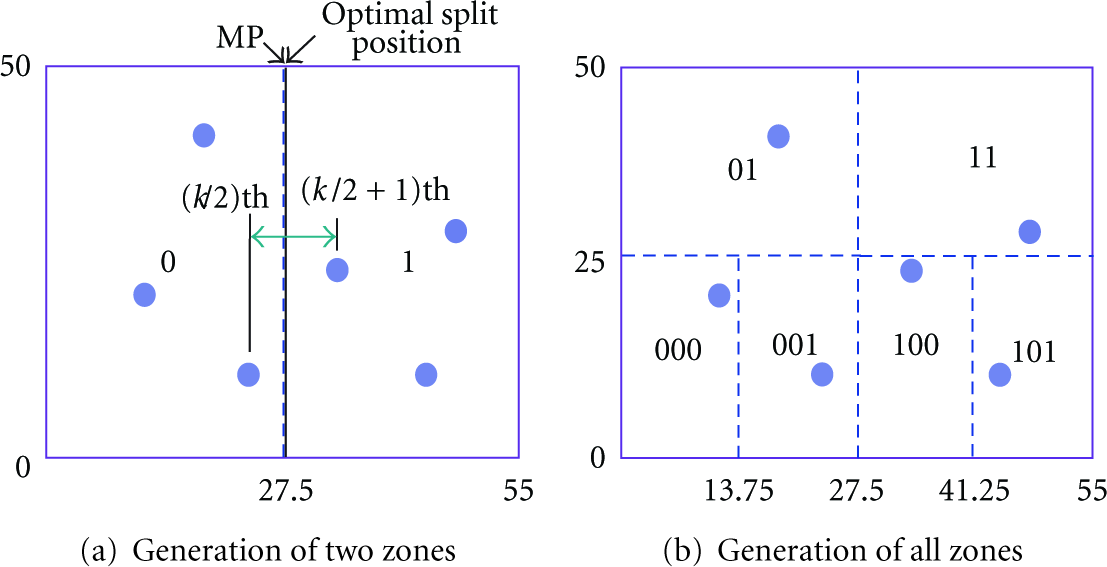
An example of zone generation.

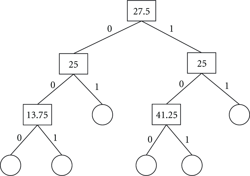
In Figure 3, the dotted-line rectangles are zones. As in Figure 3(a), the partition is first split into two non- uniform zones at position 27.5 as the optimal split position on the X axis since MP 27.5 exists between x-coordinate of the $(k / 2)$ th sensor node and x-coordinate of the $(k / 2 + 1)$ th sensor node, so that the zones have minimum difference in the number of sensor nodes and the size of the split zones. Here, the zone codes of the two split zones are 0 and 1, respectively. In Figure 3(b), all zones have been generated in the partition via the zone split process, and the original partition has a number of zones equal to the number of sensor nodes in the partition. Figure 4 shows the zone tree in the form of kd-tree for the six zones in Figure 3(b).

Figure 4

An example of a zone tree.

As in Figure 4, each node in the zone tree has the split position and two pointers for subnodes. In data storage or query processing, the zone tree is used for obtaining target sensor nodes by traversing from the root node down to the leaf nodes. In the zone tree traversal, if the zone is the left (lower) one, then the zone separator bit is set to 0 and goes down to the left lower node, and if the zone is the right (upper) one, then the zone separator bit is set to 1 and goes down to the right lower node. As the diagonal coordinates of a partition are obtained from the partition tree, the diagonal coordinates of a zone can be obtained from the zone tree.

In NUNS, the entire zone split is performed by a sensor node, called the zone split node (ZSN), in each partition. NUNS selects a sensor node as ZSN, whose location is nearest to centroid of each partition. The split process of ZSN is as follows. ZSN requests the locations of sensor nodes by flooding requests to all sensor nodes in the partition and performs the zone split process according to the zone generation algorithm by using responds from all sensor nodes in its partition. Finally, ZSN floods the zone tree as a result of the zone split process to all sensor nodes in its partition. Since each partition has as many zones as the number of sensor nodes that it contains and $2^{i}$ partitions exist in the sensor network, where i is the level of the partition tree, the time complexity for constructing the zone trees is $O (d / 2^{i} \sqrt{n})$ , where n and d are the number of sensor nodes and the diameter of the sensor network, respectively. Algorithm 2 shows the zone generation algorithm in NUNS.

Algorithm 2: Zone generation algorithm.

GenerateZone(partition, axis)

Begin

(l) i ← 0; loc ← null; initZone(zArray[2]);

(2) loc ← FindSplitpoint(partition, axis);

(3) SplitZone(partition, zArray, axis, loc);

(4) UpdateZoneTree(zArray, axis, loc);

(5) if(axis) then

(6) axis ← 0;

else

(7) axis ←1;

end if

(8) for i from 0 to1 do

(9) if(GetSensorNumber(zArray[i]) > 1) then

(10) Generate Zone (zArray [i].zone, axis);

end if

end for

End

In the zone generation algorithm in Algorithm 2, input parameter partition is the partition to be split and axis is the split axis. Line 1 initializes variable loc for storing the optimal split position of the split axis and structure zArray for storing information on split zones. Line 2 calculates the optimal split position of the split axis that minimizes the difference in the number of sensor nodes and in the size of split zones and stores it in variable loc. Line 3 splits partition nonuniformly using the split axis and the optimal split position, and it stores information on the split zones in structure zArray. Line 4 generates the zone tree for the split zones, and Lines 5~7 switch the current split axis into the other for splitting partition alternately between the X axis and Y axis. If each of the two zones obtained from splitting partition has two or more sensor nodes, then Lines 8~10 repeat the zone split process. Otherwise, it stops splitting the zones.

Compared to DIM that performs a uniform split, it seems that partition and zone generation in NUNS brings about overhead to store information on a nonuniform split. However, because each sensor node has information on the zones within the partition to which it belongs, NUNS can reduce the storage overhead for the index management and does not have orphan zones. Furthermore, since the nonuniform split of the sensor network is performed periodically in NUNS, the sensor network can operate normally even if the sensor nodes are added or deleted. And compared to KDDCS that performs storage load balancing of sensor nodes, though load balancing in NUNS is not sufficient, it can reduce the storage overhead of hot-spots and, unlike KDDCS, does not need additional routing overhead for storing data, processing queries, and maintaining kd-tree.

3.3. Data Storage

In NUNS, data measured in a partition are stored and managed in the sensor nodes within the partition. If a sensor node measures data, then the sensor node hashes the data value to find a zone that contains a sensor node for storing the data using the zone tree for the partition, and it then stores the data in the sensor node of the zone. Here, the corresponding zone is determined by traversing the zone tree from the root node down to leaf nodes and comparing the split axis and the optimal split position of the split axis stored in the nodes with the measured data value.

For example, let us assume that data have two attributes, each of which can have a value between 0 and 1. Then, because the ranges of the X axis and Y axis of a partition are mapped to the ranges of data attribute values in NUNS, the values mapped the X axis and Y axis of the partition range between 0 and 1. In Figure 5, the numbers on the two lines in parallel with the coordinate axes show the values of the attributes normalized between 0 and 1.

Figure 5

An example of data storage.

In our case, if $〈$ 0.3, 0.8 $〉$ is the data measured by sensor node A as shown in Figure 5, then zone tree traversing for the data is performed as follows. First, from the root node, because the value 0.3 of the first attribute in the measured data is smaller than the mapping value 0.5 corresponding to the optimal split position 27.5 of the split X axis, then it goes down to the left child node. Then, because the value 0.8 of the second attribute in the measured data is larger than the mapping value 0.5 corresponding to the optimal split position 25 of the split Y axis, it goes down to the right child node. At this time, because the accessed lower node is a leaf node, its zone code is determined. The zone code is 01, and the data is stored in the sensor node within the zone indicated by the zone code. Figure 5 shows an example of data stored in this way.

As shown in Figure 5, data measured in a partition is stored in the sensor nodes within the partition, and this can prevent the concentration of data storing load on a specific sensor node when data of the same value occur frequently in the sensor network. In addition, this can reduce the communication cost for storing data because the distance between the sensor node measuring data and the sensor node storing the data is shortened. Moreover, as every zone has one sensor node in NUNS, there is no orphan zone that can exist in DIM, and this can reduce the cost of unnecessary routing. Algorithm 3 shows the data storing algorithm in NUNS.

Algorithm 3: Data storing algorithm.

StoreData(loc, data)

Begin

(1) n, i ← 0; ctz, tl ← null; dl ← loc;

(2) ctz ← HashData(dara);

(3) if(CheckInternalSensor(dl)) then

(4) AddData(data);

else

(5) n ←CheckNeighbor(dl);

(6) for i from 1 to n do

(7) tl ← GetNeighborLocation(i);

(8) if(IsNearest(ctz, tl, dl) then

(9) dl ← tl;

end if

(10) if(dl == loc) then

(11) dl ← RightRoutingQuery(loc, ctz);

end if

end for

(12) StoreData(dl, data);

end if

End

In the data storing algorithm shown in Algorithm 3, input parameter loc is the location of the current sensor node that generates data, and data is the data to be stored. Here, data can contain one or more attribute data. Line 2 hashes data and determines the centroid of the target zone using the zone tree. Lines 3~4 check whether or not the target zone contains the current sensor node. If it does, since the current sensor node is the target sensor node for storing the data, then data is stored and the data storing algorithm terminates. If not, then Line 5 gets the number of neighbor sensor nodes in order to find a sensor node for transferring the data to the target zone, and Lines 6~9 find the location of the sensor node nearest to the target zone among the neighbor sensor nodes and stores the location in variable $d l$ . If it is not found, then Lines 10~11 switch the routing path to the right and get the location of the sensor node there, and they store the location in variable $d l$ . Line 12 calls StoreData() function with the location of the sensor node and data to be stored.

3.4. Query Processing

In NUNS, data measured in a partition is stored and managed in the sensor nodes within the partition. Therefore, if a query occurs in a sensor node, then the query should be transferred to all sensor nodes, which will process the query, in all the partitions of the sensor network. In order to transfer the query to all partitions, the sensor node in which the query occurred should know the locations of all partitions. The locations of all partitions can be determined by traversing the partition tree. If a query reaches any sensor node of a partition by using the partition tree, the query should be transferred to the target sensor node in the partition, which will process the query. Figure 6 shows an example of a query that is transferred to the four partitions of Figure 1(b). Numbers on the two lines in parallel with the coordinate axes show the values of the attributes normalized between 0 and 1.

Figure 6

An example query transfer.

As in Figure 6(a), sensor node A finds the centroids of all partitions using the partition tree and transfers query $〈$ 0.3–0.7, 0.8–0.9 $〉$ to them. The query from sensor node A is transferred first to sensor nodes B, C, and D in the partitions. In addition, as shown in Figure 6(b), each of sensor nodes A, B, C, and D hashes query $〈$ 0.3–0.7, 0.8–0.9 $〉$ to generate a centroid of the target zone, finds the target sensor node in the its zone, and transfers the query to the target sensor node. In the hashing process, the query is decomposed into subqueries according to the data range of each zone, and its target zone is determined for each of the decomposed subqueries. In addition, the decomposed subquery is transferred to the sensor node in the target zone that is determined by traversing the zone tree from the root node down to the leaf nodes and by comparing the split axis and the optimal split position of the split axis stored in the nodes and the attribute values used in the query.

For example, the zone codes for query $〈$ 0.3–0.7, 0.8–0.9 $〉$ occurring in sensor node A in the left lower one among the four partitions of Figure 6(b) are determined as follows. First, from the root node in the zone tree in Figure 4, because the value of the first attribute is $〈$ 0.3–0.7 $〉$ , the query is decomposed into subqueries $〈$ 0.3–0.5, 0.8–0.9 $〉$ and $〈$ 0.5–0.7, 0.8–0.9 $〉$ based on the mapping value 0.5 corresponding to the optimal split position 27.5 of the split X axis, and they are transferred to the left and right lower nodes, respectively. In the subquery $〈$ 0.3–0.5, 0.8–0.9 $〉$ transferred to the left lower node, since the value of the second attribute $〈$ 0.8–0.9 $〉$ is larger than the mapping value 0.5 corresponding to the optimal split position 25 of the split Y axis, it goes down to the right lower node. Because the right lower node is a leaf node, its zone code becomes 01. Next, in the subquery $〈$ 0.5–0.7,0.8–0.9 $〉$ transferred to the right lower node, since the value of the second attribute $〈$ 0.8–0.9 $〉$ is larger than the mapping value 0.5 corresponding to the optimal split position 25 of the split Y axis, it goes down again to the right lower node. Because the right lower node is a leaf node, its zone code is 11. Consequently, the query is decomposed into two subqueries with zone codes 01 and 11, respectively.

In NUNS, since the measured data of a sensor network are distributedly stored among the partitions, the communication cost of sensor nodes to store the data can be reduced. However, because the queries should be transferred to all the partitions and their results should be returned to the queried sensor node, the communication cost of the sensor network can increase due to query processing. Algorithm 4 shows the algorithm for transferring a query to all partitions and returning the results.

Algorithm 4: Query transfer algorithm for partitions.

TransferPQuery(loc, query, ptroot)

Begin

(1) n, i ← 0; ctp, tl ← null; dl ← loc;

(2) ctp ← HashQuery(ptroot);

(3) while (!CheckInternalPartition(dl)) do

(4) n ← CheckNeighbor(dl);

(5) for i from 0 to n do

(6) tl ← GetNeighborLocation(i);

(7) if(IsNearest(ctp, tl, dl)) then

(8) dl ← tl;

end if

end for

(9) if(dl == loc) then

(10) dl ←RightRoutingQuery(loc, ctp);

end if

end while

(11) TransferZQuery(dl, query, ztroot);

(12) RespondResult(query);

(13) end while(ctp)

End

In the query transfer algorithm for partitions shown in Algorithm 4, input parameter loc is the location of the current sensor node that transfers a query, query is the query, and ptroot is the root node of the partition tree. Line 1 initializes all variables to be used in the algorithm. Lines 2~13 transfer the query to partitions by as many as the number of partitions in the sensor network. Line 2 generates centroids of partitions to which the query will be transferred using ptroot. Line 3 checks whether or not the partition contains the current sensor node. If it does not, then Line 4 gets the number of neighbor sensor nodes in order to find a sensor node for transferring the query. Lines 5~8 find the location of the sensor node nearest to the partition, to which the query will be transferred, among the neighbor sensor nodes and store the location in variable $d l$ . If it is not found, then Lines 9~10 switch the routing path to the right and get the location of the sensor node there, and they store the location in variable $d l$ . Line 11 calls TransferZQuery() function with the location of the sensor node stored in variable $d l$ and query to be transferred to find the target sensor node in the corresponding partition.

Algorithm 5 shows the algorithm for transferring a query to the target sensor nodes in zones and processing the query.

Algorithm 5: Query transfer algorithm for zones.

TransferZQuery(loc, query, ztroot)

Begin

(1) n, i ← 0; ctz, tl ← null; dl ← loc;

(2) ctz ← HashQuery (ztroot);

(3) if(CheckInternalPartition(dl)) then

(4) RespondResult(query);

else

(5) n ← CheckNeighbor(dl);

(6) for i from 0 to n do

(7) tl ← GetNeighborLocation(i);

(8) if(IsNearest(ctz, tl, dl)) then

(9) dl ← tl;

end if

end for

(10) if(dl == loc) then

(11) dl ← RightRoutingQuery(loc, ctz);

end if

(12) TransferZQuery(dl, query, ztroot);

end if

(13) end while (ctz)

End

In the query transfer algorithm for zones shown in Algorithm 5, input parameter loc is the location of the current sensor node that transfers a query, query is the query, and ztroot is the root node of the zone tree. Line 1 initializes all variables to be used in the algorithm. In case the range of the attribute values of the query covers multiple zones, Line 2 decomposes the query according to the zones of the corresponding partition and generates the centroids of zones to which the query will be transferred using ztroot. Line 3 checks whether or not the zone contains the current sensor node, and if it does, then the query is processed in the current sensor node. If it does not, then Line 5 gets the number of neighbor sensor nodes in order to find a sensor node for transferring the query. Lines 8~9 find the location of the sensor node nearest to the target zone among the neighbor sensor nodes and store the location in variable $d l$ . If it is not found, then Lines 10~11 switch the routing path to the right and get the location of the sensor node there, and they store the location in variable $d l$ . Line 12 calls TransferZQuery() function with the location of the sensor node stored in variable $d l$ and the query to be transferred.

4. Performance Evaluation

This section compares performance in terms of data storage and query processing among NUNS proposed in this paper, DIM which is superior to GHT and DIFS, and KDDCS which efficiently performs storage load balancing of sensor nodes. In the performance evaluation, we used a computer system with Intel Core2 CPU 2.13 GHz, 2 GB RAM, and Windows XP Professional. In addition, we simulated the sensor networks of sizes ranging from 200 to 1,000 sensor nodes, each having an initial energy of 10,000 units, a radio range of 40 m, and a storage capacity of 20 units. Especially, the locations of the sensor nodes were arbitrarily deployed into the sensor network boundary.

4.1. Data Storage Cost

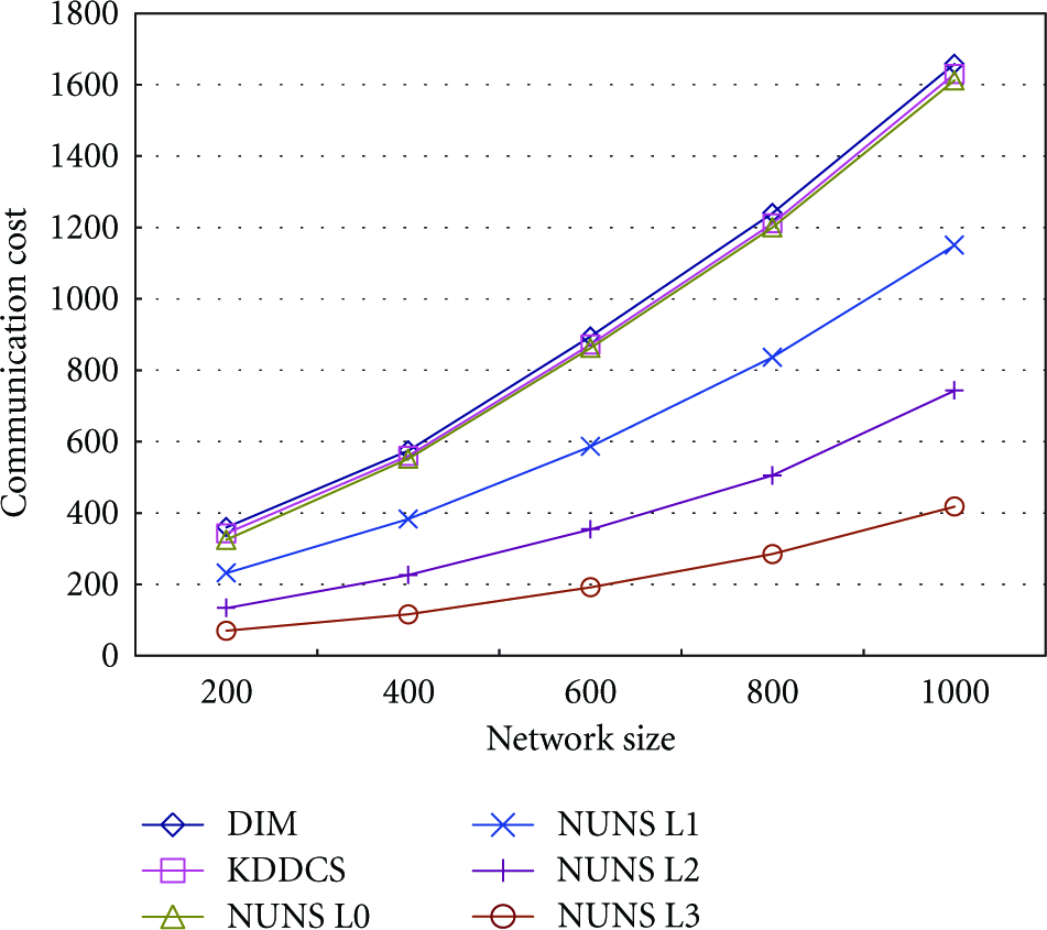
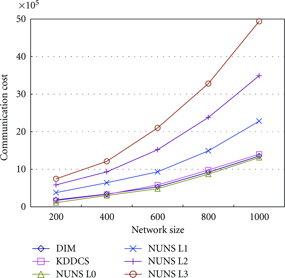
In this section, we compared NUNS with DIM and KDDCS in terms of communication cost for storing measured data in a sensor network. In the experiment, each sensor node generated three data with two attributes randomly while increasing the size of the sensor network by increasing the number of sensor nodes from 200 up to 1,000. Especially, in order to impose a storage hot-spot on the sensor network, for each network size, we generate a series of hot-spots where a percentage of 10% to 80% of the data fell into a percentage of 5% to 10% of the range of each attribute value. Figures 7 and 8 show the data storage cost in the sensor network and at the hot-spot, respectively. NUNS L0, NUNS L1, NUNS L2, and NUNS L3 mean that the split is performed 0, 1, 2, and 3 times, respectively (i.e., they have 1, 2, 4, and 8 partitions, resp.).

Figure 7

Data storage cost in sensor network.

Figure 8

Data storage cost at hot-spot.

As shown in Figure 7, as the size of the sensor network becomes larger, the communication cost for data storage of NUNS with many partitions is more efficient than that of DIM and KDDCS. This is because by storing the data value measured in a partition in a sensor node within the partition in NUNS, the distance between the sensor node measuring data and the sensor node storing the data is shortened, and consequently the communication cost for storing data is reduced. In addition, the cost of unnecessary routing can be avoided in NUNS as a partition is split nonuniformly into zones and there is no orphan zone, unlike DIM. Especially, the communication cost of KDDCS can increase since additional overhead for rebalancing kd-tree is needed in KDDCS.

Similar to the data storage cost of the sensor network in Figure 7, as the size of the sensor network becomes larger, the communication cost of data storage at the hot-spot in NUNS with many partitions also appeared more efficient than that in DIM and KDDCS, as is shown in Figure 8. This is because by storing the data value measured in the sensor network distributedly among the partitions in NUNS, the storage load in the hot-spot can be reduced, and by splitting each partition into zones by minimizing the difference in the size of the split zones in NUNS, load concentration on a specific zone with a large processing region can be prevented. Especially, KDDCS can consume additional energy to move data of the hot-spot to neighbors for load balancing, which shorten the lifetime of the hot-spot.

4.2. Query Processing Cost

We compared NUNS with DIM and KDDCS in terms of communication cost for query processing in the sensor network. In the experiment, each sensor node generated two range queries with two attributes at random while increasing the size of the sensor network with the number of sensor nodes from 200 up to 1,000. For each network size, the queries were executed within 10% of the maximum range of the attribute values. Figures 9 and 10 show the query processing cost in the sensor network and at the hot-spot, respectively.

Figure 9

Query processing cost in sensor network.

Figure 10

Query processing cost at hot-spot.

As shown in Figure 9, with the increase of sensor network size, NUNS with 1 partition was a little more efficient in terms of communication cost for query processing than DIM and KDDCS. However, NUNS with 2, 4, or 8 partitions showed a higher communication cost for query processing than DIM and KDDCS. This is because the communication cost for query processing particularly increases when the number of partitions becomes larger, since a query should be transferred to the target sensor nodes of all the partitions and its result should be returned to the sensor node in which the query occurred.

As shown in Figure 10, the communication cost for query processing at the hot-spot in NUNS with 1 partition appeared less efficient than that of KDDCS and more efficient than DIM, but the cost in NUNS with 2, 4, or 8 partitions was more efficient than that of DIM and KDDCS. This is because NUNS can distribute the storage load of the hot-spot among partitions in the sensor network and consequently reduce the transfer cost of query results at the hot-spot. Therefore, the optimal number of partitions in NUNS should be determined in consideration of the frequency of data storage and the frequency of query processing in the data-centric storage sensor network.

4.3. Communication Cost according to Cost Ratio

This section experimented on the communication cost of the sensor network and that of the hot-spot according to the ratio of the frequency of data storage to the frequency of query processing. That is, we compared NUNS with DIM and KDDCS in terms of communication cost while changing the ratio from 1 : 1 up to 100 : 1. In the experiment, the communication range of the sensor nodes was set to 40 m and 1,000 sensor nodes were used. In addition, 100~10,000 data with two attributes and 100 range queries with two attributes were generated at random. For each network size, the queries were executed within 10% of the maximum range of the attribute values. Figures 11 and 12 show the communication cost according to the ratio in the sensor network and at the hot-spot, respectively.

Figure 11

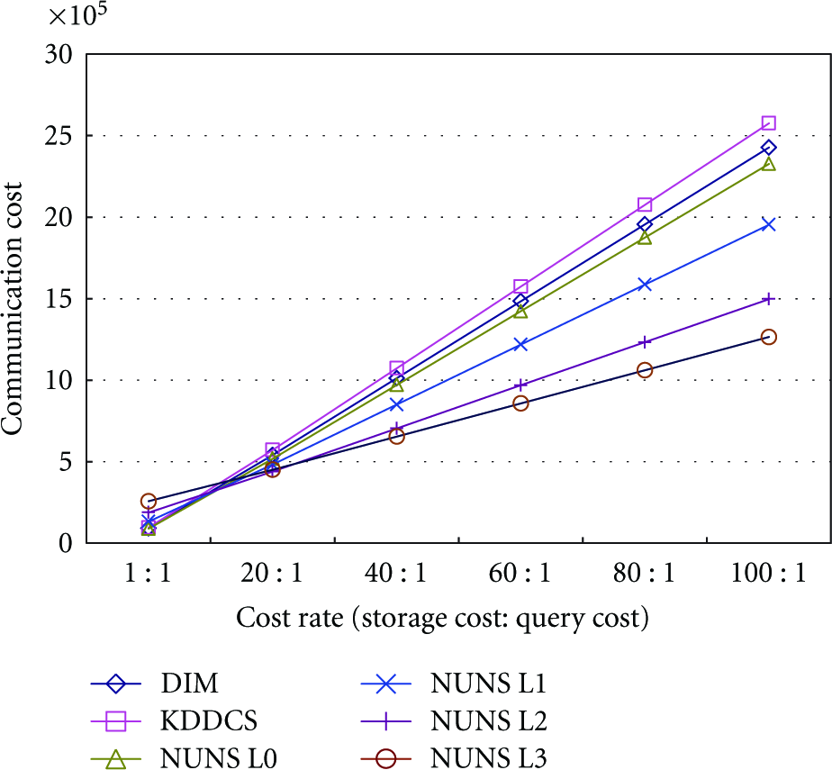
Communication cost in sensor network.

Figure 12

Communication cost at hot-spot.

As shown in Figure 11, in comparison with DIM and KDDCS, NUNS with 1 partition was most efficient in terms of communication cost of the sensor network when the ratio of the frequency of data storage to the frequency of query processing was 1 : 1~20 : 1, and NUNS with 8 partitions was most efficient when the ratio was 40 : 1~100 : 1. In addition, the communication cost efficiency of NUNS with the large number of partitions is expected to be higher than DIM and KDDCS as the frequency of data storage becomes larger than the frequency of query processing. This is because with the increase in the number of partitions in NUNS, the cost of data storage decreases but the cost of query processing increases, and consequently the decrease in the cost of data storage becomes relatively larger than the increase in the cost of query processing, as the frequency of data storage becomes higher than the frequency of query processing.

Similar to the communication cost of the sensor network in Figure 11, in comparison with DIM and KDDCS, the communication cost at the hot-spot as shown in Figure 12 also revealed the efficiency of NUNS with a large number of partitions as the frequency of data storage becomes higher than the frequency of query processing.

The results of the experiments above show that in all cases, NUNS with one partition is more efficient for data storage and query processing than DIM and KDDCS. In addition, with the increase in the number of partitions in NUNS, the cost of query processing increases, but the cost of data storage decreases. Accordingly, we expect to enhance the energy efficiency of the sensor network by using NUNS in the data-centric storage sensor network where data values are stored frequently.

5. Conclusions

In the data-centric storage sensor network, the sensor nodes for data storage are determined by the value of measured data, and thus if data have the same value frequently, then the load is concentrated on a specific sensor node and the sensor node consumes energy rapidly. In addition, if the sensor network is expanded through the addition of new sensor nodes, then the distance between the senor node measuring data and the sensor node storing the data grows longer, and this increases the communication cost in data storage and query processing. Therefore, it is important to enhance the energy efficiency of the sensor network by distributing the load among the sensor nodes and by reducing the communication cost resulted from expanding the sensor network.

To solve these problems, this paper proposed a nonuniform network split method, called NUNS, for the data-centric storage sensor network. In order to distribute the load among sensor nodes and reduce the communication cost for data storage and query processing resulted from expanding the sensor network, NUNS splits a sensor network into partitions of nonuniform sizes and stores data that occurs in each partition and is managed by sensor nodes within the partition. In addition, for preventing load concentration on a specific sensor node and reducing the cost of unnecessary routing, NUNS splits each partition into zones of nonuniform sizes by as many as the number of sensor nodes in the partition. Lastly, this paper proved through experiments that NUNS is more energy efficient than DIM and KDDCS in the data-centric storage sensor network where data are stored more frequently.

Footnotes

Acknowledgment

This research was supported by a Grant (07KLSGC05) from Cutting-edge Urban Development—Korean Land Spatialization Research Project funded by Ministry of Land, Transport and Maritime Affairs of Korean Government.

References

Draper

S. C.

Wornell

G. W.

Side information aware coding strategies for sensor networks

IEEE Journal on Selected Areas in Communications 2004 22 6 966 976

2-s2.0-4344695233

10.1109/JSAC.2004.830875

Lee

B. S.

Wang

X. S.

Aggregation in sensor networks with a user-provided quality of service goal

Information Sciences 2008 178 9 2128 2149

2-s2.0-39749173666

10.1016/j.ins.2008.01.003

Karp

Kung

H. T.

GPSR: greedy perimeter stateless routing for wireless networks

Proceedings of the 6th Annual International Conference on Mobile Computing and Networking

August 2000

Boston, Mass, USA

243 254

2-s2.0-0034547115

Madden

Franklin

M. J.

Hellerstein

J. M.

Hong

TAG: a tiny aggregation service for ad-hoc sensor networks

Proceedings of the 5th Symposium on Operating System Design and Implementation

2002

131 146

Ren

Liang

Energy and quality aware query processing in wireless sensor database systems

Information Sciences 2007 177 10 2188 2205

2-s2.0-33847619375

10.1016/j.ins.2006.12.017

Doss

Mak

Chowdhury

Improving the QoS for information discovery in autonomic wireless sensor networks

Pervasive and Mobile Computing 2009 5 4 334 349

2-s2.0-67349145919

10.1016/j.pmcj.2008.09.006

Kim

Y. J.

Govindan

Hong

Multi-dimensional range queries in sensor networks

Proceedings of the 1st International Conference on Embedded Networked Sensor Systems

November 2003

Los Angeles, Calif, USA

63 75

2-s2.0-4243197464

Mainwaring

Polastre

Szewczyk

Culler

Anderson

Wireless sensor networks for habitat monitoring

Proceedings of the 1st ACM International Workshop on Wireless Sensor Networks and Applications

September 2002

Atlanta, Ga, USA

88 97

2-s2.0-0036986465

Liu

Huang

Zhang

Balancing push and pull for efficient information discovery in large-scale sensor networks

IEEE Transactions on Mobile Computing 2007 6 3 241 251

2-s2.0-33847708378

10.1109/TMC.2007.34

10.

Ratnasamy

Karp

Yin

Estrin

Govindan

Shenker

GHT: a geographic hash table for data-centric storage

Proceedings of the 1st ACM International Workshop on Wireless Sensor Networks and Applications

September 2002

Atlanta, Ga, USA

78 87

2-s2.0-0036983290

11.

Ratnasamy

Estrin

Govindan

Karp

Shenker

Data-centric storage in sensornets

Proceedings of the 1st ACM SIGCOMM Workshop on Hot Topics in Networks

2003

137 142

12.

Ratnasamy

Karp

Shenker

Estrin

Govindan

Yin

Data-centric storage in sensornets with GHT, a geographic Hash Table

Mobile Networks and Applications 2003 8 4 427 442

2-s2.0-0042564491

10.1023/A:1024591915518

13.

Ganesan

Estrin

Heidemann

Dimensions: why do we need a new data handlingarchitecture for sensor networks?

Proceedings of the 1st ACM Workshop on Hot Topics in Networks

2002

143 148

14.

Greenstein

Estrin

Govindan

Ratnasamy

Shenker

DIFS: a distributed index for features in sensor networks

Proceedings of the 1st IEEE International Workshop on Sensor Network Protocols and Applications

May 2003

Anchorage, Alaska, USA

163 173

10.1109/SNPA.2003.1203367

15.

Lai

Wang

Chen

Energy-efficient robust data-centric storage in wireless sensor networks

Proceedings of the International Conference on Wireless Communications, Networking and Mobile Computing

September 2007

Shanghai, China

2735 2738

2-s2.0-38049052965

10.1109/WICOM.2007.679

16.

Sharifzadeh

Shahabi

Supporting spatial aggregation in sensor network databases

Proceedings of the 12th ACM International Symposium on Advances in Geographic Information Systems

November 2004

Washington, DC, USA

166 175

2-s2.0-19544375417

17.

Aly

Pruhs

Chrysanthis

P. K.

KDDCS: a load-balanced in-network data-centric storage scheme for sensor networks

Proceedings of the 15th ACM Conference on Information and Knowledge Management

November 2006

Arlington, Va, USA

317 326

2-s2.0-34547622100

10.1145/1183614.1183662

18.

Aly

Chrysanthis

P. K.

Pruhs

Decomposing data-centric storage query hot-spots in sensor networks

Proceedings of the 3rd Annual International Conference on Mobile and Ubiquitous Systems (MobiQuitous ′06)

July 2006

San Jose, Calif, USA

1 9

2-s2.0-50249107808

10.1109/MOBIQW.2006.361728

19.

Aly

Morsillo

Chrysanthis

P. K.

Pruhs

Zone sharing: a hot-spots decomposition scheme for data-centric storage in sensor networks

Proceedings of the 2nd International Workshop on Data Management for Sensor Networks

August 2005

21 26

2-s2.0-77954445300

10.1145/1080885.1080890

NUNS: A Nonuniform Network Split Method for Data-Centric Storage Sensor Networks

Abstract

1. Introduction

2. Related Works

3. NUNS (Non-Uniformed Network Split)

3.1. Partition Generation

Algorithm 1: Partition generation algorithm.

3.2. Zone Generation

Algorithm 2: Zone generation algorithm.

3.3. Data Storage

Algorithm 3: Data storing algorithm.

3.4. Query Processing

Algorithm 4: Query transfer algorithm for partitions.

Algorithm 5: Query transfer algorithm for zones.

4. Performance Evaluation

4.1. Data Storage Cost

4.2. Query Processing Cost

4.3. Communication Cost according to Cost Ratio

5. Conclusions

Footnotes

Acknowledgment

References