
Abstract
Optimal sensor placement (OSP) technique plays a key role in the structural health monitoring (SHM) of large-scale civil infrastructures. This paper outlines an overview of current research and development in the field of OSP problems in a perspective of both researchers and engineers. The paper begins with a definition of the model of sensor placement and provides the basic issues covering relevant methodologies. The primary evaluation criteria and main sensor placement methods are then discussed in details. Following that, the linkage between several influential sensor placement methods is described. Finally, existing problems and promising research efforts in the OSP problem of civil SHM are discussed.
1. Introduction
Today, there are many more large-scale civil infrastructures than in the past. These structures are susceptible to random vibrations in its long service period; whether it is from changes in temperature, severe wind gusts, torrential rain, strong earthquake tremors, or abnormal loads such as explosions [1–3]. The coupling effects between these natural or man-made factors make the problem even more complicated. Although the routine visual inspection is effective in some cases, its effectiveness in finding the possible defects in time is questionable. Therefore, it is imperative that a continuous structural health monitoring (SHM) system be developed. The SHM systems are generally envisaged to [4]: (i) validate the design assumptions and parameters with the potential benefits of improving design specifications and guidelines for future similar structures; (ii) detect anomalies in loading and response, and possible damage/deterioration at an early stage to ensure the structural and operational safety; (iii) provide the real-time information for the safety assessment immediately after disasters and extreme events; (iv) provide the evidence and instruction for planning and prioritizing the structural inspection, rehabilitation, maintenance, and repair; (v) monitor the repair and reconstruction with the view of evaluating the effectiveness of maintenance, retrofit and repair work; (vi) obtain the massive amount of in situ data for the leadingedge research in structure engineering, such as wind- and earthquake-resistant designs, novel structural types, and smart material applications.
A typical SHM system includes three major components: a sensor system, a data processing system (including the data acquisition, transmission, and storage), and a health evaluation system [5]. The sensors utilized in the SHM are required to monitor not only the structural status including stress, displacement, acceleration, but also those influential environmental parameters, such as wind speed, temperature, humidity, soil condition of its foundation. Generally, the more locations of sensors placed on a structure are, the more detailed information of the structure could be obtained. In addition, advances in sensing technology have also enabled the use of large numbers of sensors for the SHM. However, high costs of data acquisition systems (including development, purchase and maintenance costs for the sensors, as well as resource and communication costs) and accessibility limitations constrain in many cases the wide distribution of a large number of sensors on a structure. Especially, many structures have to be tested under operational conditions, in which the sensors are not easily amenable to be removed or changed. In such cases, a practical question that naturally arises is how to select a set with a minimum number of sensor locations from all possibilities, such that the data collected can provide adequate information for the identification of the structural behavior. Otherwise, incomplete structural and environmental characteristics may be measured and an accurate SHM assessment will be impossible. Generally, the design of a sensor network for the SHM system excepts identifying the rational number and location of sensors in order to fulfill specified performance requirements within a set of system constraints. Another area of interest is sensor network robustness, which aims at maintaining the stability of the sensor network when some sensors malfunction [6]. The development and implementation of various kinds of sensor placement methods capable of fully achieving the above objectives and benefit are still challenging at present, and need well-coordinated interdisciplinary research for full adaptation of innovative technologies developed in other disciplines to applications in the civil engineering community. Actually, the optimal sensor placement (OSP) has been a subject of important international research in recent years. The research in this subject covers sensing, structural dynamics, information technology, optimization theory, and so forth [7, 8]. The current challenges for the OSP method are being identified as intelligent and efficient algorithms, evaluation criteria for different sensor placement methods, inherent relationship between different sensor placement methods, and uncertainty, sensitivity, reliability, and redundancy in sensor networks, and so forth.
In this paper, a brief overview of the OSP problem is given in Section 2; a detailed discussion of current status of evaluation criteria and sensor placement methods are provided in Sections 3 and 4, respectively; the comparison of several influential sensor placement methods is described in Section 5, and the concluding remarks are given in Section 6. This paper is not intended to be encompassing in terms of directly comparing the various techniques against each other and assessing their performance. Rather, the review is based on categorizing salient features of these approaches and the desirability of certain features when they are applied to SHM systems.
2. Objective of Sensor Placement for SHM
The OSP issue is important in cases where the properties of a structure, described in terms of continuous functions, need to be identified using discrete sensor information. Thus, the sensor placement optimization is a kind of combinatorial optimization problem that can be generalized as “given a set of n candidate locations, find m locations, where

For a structure that has simple geometry, or smaller number of degrees of freedom (DOF), experience and a trial-and-error approach may suffice to solve the problem. For a large-scale complicated structure, whose finite element model may have thousands, tens of thousands, and even hundreds of thousands of DOFs, an exhaustive search would be extremely time consuming or even impossible. Thus, a systematic and efficient approach is needed to solve such a computationally demanding problem.
2.1. Model for Sensor Placement in Structural Dynamics
The sensor placement problem can be investigated from uncoupled modal coordinates of governing structural equations as follows [9]:
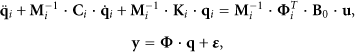
where,
2.2. Basic Issues Regarding Sensor Placement
Sensor placement problem described in (2) is, essentially, divided into three aspects [10]. Firstly, what is the least number of sensors required to be installed in a structure for a successful dynamic testing? Secondly, where should these sensors be installed, including those additional ones if available? And if these additional sensors are available, should they be installed as redundant sensors or place them in other positions? Lastly, how could the effectiveness of different sensor placement methods be evaluated?
In fact, these three aspects are intervening with each other, and the first problem is partly resolved. It is known that the minimum number of sensors to be instrumented could not be less than the number of mode shapes to be identified, which is determined by the observability of the structure. Moreover, the practical number of sensors, which is limitedly preset before test due to the availability of instruments, is usually larger than the minimum number because of the requirement to visualize the identified mode shapes (i.e., the identified mode shapes are dependent on each other and one or more of them can be determined by a combination of others) [11]. The second problem is the core one that has attracted the majority of research interest, which depends largely, however, on the third aspect. For the limited number of sensors available, the problem is the development of a suitable sensor placement performance measure to be optimized and the selection of an appropriate method with which it can be optimized. Some approaches require a single calculation to be performed, some are iterative, and many others take the form of an objective function to which an optimization technique must be applied. The third aspect includes several possibilities for assessing the performance of chosen sensor sets. If the economical issues were not considered, only after the last two aspects are clearly understood, it was then possible to know exactly the required number of sensors to be installed.
3. Criteria to Evaluate Suitability of Sensor
It should be noted that a good method for sensor placement in a particular application is not necessarily good for another project. That means the effectiveness of a certain sensor placement method depends on the evaluation criteria to some extent. A criterion stresses one perspective whereas another pays more attention to another aspect. Compromises need to be made if one or several of the criteria are to be used in dynamic testing. In this section, some influential criteria are discussed both from historical points of view and from their impacts on practices and the development of sensor placement theory. Of course, bias and omissions could not be avoided for such a daunting task because of personal knowledge. Descriptions have been kept mathematically light intentionally; full descriptions of the criteria may be found in the references.
(1) Modal Assurance Criterion (MAC)
As known, the measured mode shape vectors have to be as linearly independent as possible, which is a basic requirement to distinguish measured or identified modes. Moreover, the linear independency is also particularly important when the test results are to validate or to update the FE model. The larger space angles among the measured modal vectors should be guaranteed while choosing measuring points in order to keep the original properties of the structure if possible. Carne and Dohmann (1995) [12] thought that the MAC was an ideal scalar constant relating the causal relationship between two modal vectors

where,
The element values of the MAC matrix range between 0 and 1, where zero indicates that there is little or no correlation between the off-diagonal element
(2) Singular Value Decomposition Ratio (SVDR)
The singular value decomposition of mode shape matrix specified at a certain DOF provides another measure to the chosen sensor locations [13]. The method evaluates the ratio of the largest to the smallest singular value of the mode shape matrix:

where,
The smaller the ratio, the better the choice of sensor locations. There are three reasons to adopt the SVDR criteria: namely, mode orthogonality, the condition for mode expansion, and the observability of the modes [14]. The lower limit of the SVDR is one in the case that the mode shapes are orthogonal, which is an ideal situation. This criterion can also be termed as the condition criteria since the SVDR of a truncated mode shape matrix is nothing else, but its condition number.
(3) Measured Energy per Mode
Since the kinetic energy of a structure is usually not evenly distributed into the modes of the structure, the measured DOFs are expected to capture a large part of the total kinetic energy of the structure, and the energy contained in the measured DOFs for each mode should be a significant portion of that mode to satisfactorily measure the modes. It is based on the traditional heuristic visual inspection, which is to visually inspect the response of a structure, to examine the mode shapes of interest, and to select locations with high amplitudes of responses. This criterion helps to select those sensor positions with possible large amplitudes, and to increase the signal to noise ratio, which is critical in harsh and noisy circumstances.
(4) Fisher Information Matrix (FIM)
The criterion of the FIM results from minimizing the covariance matrix of the estimate error for an efficient unbiased estimator from the perspective of statistics. It relates also to the information contained in the measured responses from the viewpoint of information community:

Therefore, the procedure using this criterion for selecting the best sensor placements is to unselect candidate sensor positions such that the FIM is maximized. In practice, three variants of the FIM are used, the determinant, the trace, as well as the minimum singular value of the FIM, which are maximized to increase the information or to decrease the uncertainties of the estimates. What need to be mentioned is that these three variants are just different norms of a matrix, that means, different sensor placement methods based on these variants of the FIM will yield similar, if not the same, results for most cases [15, 16].
(5) Probability-Based Damage Detection Criterion
Since any SHM issue is fundamentally a detection problem in its simplest execution, Flynn and Todd [17] developed a global optimality criterion within a detection theory framework that seeks to optimize a given sensing network resource allocation for minimizing the expected appearance of type I or type II error.
The first global performance measure, which is called the global false alarm rate, is the expected proportion of the structural undamaged regions that will be incorrectly identified as damage, or render type I error. It can be expressed as

where,
The second global performance measure, which is labeled the global detection rate, is the expected proportion of the structural damaged regions that will be correctly identified as damaged. This is equivalent to the complement of the proportion of the structure to exhibit type II error. It can be expressed as

where,
(6) Mean Square Error (MSE)
For randomly vibrating structures, the problem of estimating the optimal sensor locations can be chosen to minimize the total, averaged over all prediction points, mean square error (MSE) of the response prediction [18]. The MSE
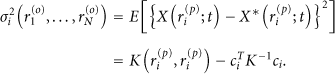
The MSE depends on the location of the observation points
(7) Information Entropy (IE)
In experimental design, it is desirable to design the sensor configuration such that the resulting measured data are most informative about the structural model parameters selected for estimation. The information entropy (IE) as the measure of the uncertainty in the system parameters gives the amount of useful information contained in the measured data. The most informative test data are the ones that give the least uncertainty in the parameter estimates or, equivalently, the ones that minimize the IE. Thus, among all sensor configurations, the optimal sensor configuration can be selected as one that minimizes the IE [19–22]. That is
where,

where
(8) Mutual Information (MI)
The MI gives a measure of how much information one sensor location, “learns” from another [23]. If there are two sets of measurement locations, A and B, the amount of information learned by

where
If the measurement of
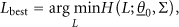
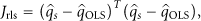
(9) Representative Least Squares Criterion (RLSC)
The RLSC derived from the representative least square method depends on both the characteristics and the actual loading situations of a structure [24]. The objective of the RLSC is to achieve the best identification of modal frequencies and mode shapes through almost unbiased estimation of modal coordinates. It selects sensor positions with the best subspace approximation of the vibration responses from the linear space spanned by the mode shapes.
where,
(10) Visualization of Mode Shape
Structural engineer must first visualize the mode shape vectors identified from modal experiments to have a first impression of the overall motion of the structure under consideration, as discussed by Carne and Dohmann [12]. This criterion has no concrete mathematical formulations not like the other criteria. It depends on the structure, and usually the points in the frame corner or middle are picked. As suggested by Pickrel [25], the number of sensors required to visualize the mode shapes is at least five times the number of mode shapes in order to provide a crude visual depiction of the shapes and avoid spatial aliasing. But modern structures composed of new materials can present unexpected modes, or complex couplings between substructures. Thus, it is not possible to design the best sensor set using this criteria prior to test because it would involve the vibratory behavior that should be already perfectly known.
4. Development of Sensor Placement Method
The aforementioned analyses have shown that the general sensor selection problems addressing diagnosability, or observability, reliability, and detectability are NP complete and are therefore computationally intractable. These types of issues require efficient searching solutions in order to generate acceptable results in reasonable time. Many methods have been developed for general optimized solution searches. These approaches range from applying the constraints on the objective function (evaluation criteria) to streamline the optimization process to applying the advanced artificial analysis techniques such as the genetic algorithms and simulated annealing algorithms. The point of this section is not to review each search solution but to identify the variety of algorithms available. Especially, the computational intelligent algorithms are reviewed in details due to their unique advantages for the OSP problem.
4.1. Deterministic Optimization Methods
A number of unconstrained (Newton methods) and constrained (linear and nonlinear programming) deterministic optimization methods can be used for the optimal sensor location. This includes countless methods based on the availability of gradients and Hessians. Simple deterministic techniques are sufficient for the local search, and the constrained optimization has a great degree of complexity [26]. For the structures with simple and regular shapes (like beam, plates, etc.), the optimal layout of the sensors can be obtained directly by the constrained deterministic optimization methods such as the recursive quadratic programming method, since their mode shapes and frequencies can be accurately described using the analytical expression. As aforementioned, in most of the practical problems, only discrete sites are available. The optimal selection of locations becomes an integer programming problem which is usually much more difficult and costly to solve than a continuous optimization problem. In this case, the discrete variables problem can be converted as continuous variables sometimes and then solved by the deterministic optimization methods, too. For example, Sepulveda et al. [27, 28] presented a control-augmented structural synthesis methodology in which the actuator and sensor placement is treated in terms of (0,1) variables. The combinatorial aspects of the mixed (0,1)-continuous variable design optimization problem are made tractable by combining approximation concepts with the branch and bound techniques. Sunar and Rao [29] solved the thermopiezoelectric sensor placement problem for the cantilever beamlike structures well by using the quasistatic thermopiezoelectricity equations. The advantages of the continuous optimization techniques are maturer compared with other methods, but these techniques need to use the gradient of the objective function. Thus, they are easy to fall into local optimum.
4.2. Sequential Sensor Placement Method
The sequential sensor placement (SSP) algorithm is a relative systematic and computationally efficient approach for obtaining a good sensor configuration although it cannot be guaranteed to be the optimal one [30]. The basic steps of the SSP algorithm for a fixed number of
As known, to start the SSP algorithm, the initial set of DOFs should be selected to cover the structure and areas of special interest. Carne and Dohmann [12] used intuition to determine the initial measurement set of DOFs based on experience and requirements of structural topology for the visualization of mode shapes. The original algorithm (called MinMAC) proposed by Carne and Dohrmann can be regarded as a FSSP algorithm. However, Li et al. [31] found that the maximum off-diagonal term was not monotonically decreasing with the number of sensors. The reason for such increasing contradiction is that a newly included or excluded sensor may conflict with other previously selected sensors, or even with the original intuition set. Mathematically speaking, the row vector determined at this newly included sensor position has strong linear relationship with the previous whole sensor set. To alleviate the contra-decreasing, they developed a forward-backward combinational MinMAC algorithm called the extended MinMAC algorithm. The mainly difference resides in the stopping criteria. The extended MinMAC algorithm computes further to obtain a sensor set consisting a certain number of sensors larger than the required one(s) where the original MinMAC stops. Yi et al. [32] suggested selecting the initial sensor assignment by the QR-factorization of the structural mode shape matrix. The underlying idea is to find the most linear independent rows of the modal matrix to minimize the off-diagonal terms of the MAC matrix. Papadimitriou [22] evaluated the accuracy of the sensor configurations provided by the SSP algorithms by comparing the corresponding information entropy values with those computed by genetic algorithms (GAs). He found that the BSSP and FSSP methods for predicting the maximum information entropy values depended on the number of sensors and observable modes. The performance of the two methods give approximately the same predictions for the minimum information entropy and the combined results provided by the SSP methods are in all cases better than ones provided by the GAs. In addition, the application of the SSP methods for 1 and
4.3. Combinatorial Optimization Method
Conventional gradient-based local optimization methods are unable to handle efficiently the multiple local optima and may present difficulties in estimating the global minimum. They lack reliability in dealing with the optimization problem since convergence to the global minimum is not guaranteed. In the recent years, combinatorial optimization methods based on the biological and physical analogue have been extensively used for the optimization of OSP problems due to its many advantages over the classical optimization techniques such as it is a blind search method and highly parallel. There are many interesting approaches to tackle such problems, but one of the most powerful heuristics is based on the GAs.
(1) Genetic Algorithms
The GAs try to imitate natural evolution by assigning a fitness value to each candidate solution of the problem and by applying the principle of survival of the fittest [33]. Their basic components are the representation of candidate solutions to the problem in a “genetic” form, the creation of an initial, usually random population of solutions, the establishment of a fitness function that rates each solution in the population, the application of genetic operators of crossover and mutation to produce new individuals from existing ones and finally the tuning of the algorithm parameters like population size and probabilities of performing the prementioned genetic operators [34].
In the original GA, the minimization variables must be encoded into bit strings (i.e., chromosomes with “0” and “1”). Therefore, the variables are discretized and the range of the discretization corresponds to some power of 2 (e.g., 1024). For the OSP problem, the optimization variables are the sensor locations, which could be either the spatial coordinate or the node index number. The mapping between the physical minimization variables and the chromosomes is the big difficulty in the application of GAs in addressing the OSP. The traditional coding method is the simple one dimension binary coding method which is very simple and intuitionistic [35, 36]. However, the number of sensors will be changed in the crossover and mutation, which is impractical and must be avoided [37]. In addition, the binary coding method requires increased string length and computational time especially in the large-scale structures where possible combination sensors are large. Roy and Chakraborty [38] and Chow et al. [39] suggested using the integer coding method to get over the problem. Huang et al. [40] proposed a kind of dual-structure coding approach to overcome the problem. In this coding method, the individual chromosome is composed of two rows, the upper row denotes the append code and the lower row represents the variable code. The crossover and mutation only operate on upper append code and the lower variable value of offspring is fixed which means the number of sensors could be unchanged. Different genetic operators, such as force mutation [41], filter operator [42], partially matched crossover (PMX) [43], have also been used in order to overcome these faults although the process of these particular genetic operators are complex and the computational efficiency is relatively low. Kang and Xu [44] adopted the partheno-genetic operators to sensor placement which only changed the order of the chromosome but never changed the sensor numbers. This is quite suitable to the OSP because the sensor number should be invariable during the optimization process. Considering the number of the DOF is enormous in the large-scale structures, the requirement for the large storage space is increased to save the optimal solutions, Liu et al. [45] presented a decimal two-dimension array coding approach instead of binary coding method to code the solutions. Numerical results showed that the dissipative storage space of the decimal two-dimension array coding method was minimal among them compared to the binary coding methods.
It should be noticed that, due to the nature of the GA's method, the number of iterations required for a guaranteed convergence is usually dependent on the size of the population and the searching space being used [46, 47]. For a given population size, the larger the searching space, the more the number of iterations needed to reach a converged solution with confidence. In other words, the higher confidence usually requires the number of iterations large enough, or multiple runs of the GAs process [48]. Thus, another drawback of GAs is that it may spend much time when meeting a relative large size of the searching space which is constrained by the number of nodes on the FEM mesh excluding the constrained nodes and the vibration nodes of the selected modes. Some attempts have been made to overcome this fault. For example, Javadi et al. [49] presented a hybrid intelligent GA which was based on a combination of neural network and GA. Hwang and He [50] used simulated annealing and adaptive mechanism to insure the solution quality and to improve the convergence speed. In order to improve the convergence speed and avoid premature convergence, some improved GAs also been adopted to sensor placement problems, such as the generalized genetic algorithms (GGA) [51, 52] which were based on some famous modern biological theories such as the genetic theory by Morgan, the punctuated equilibrium theory by Eldridge and Gould, and the general system theory by Bertalanffy, so it is superior in biologics to the classical GA, the elite genetic algorithms (EGA) [53], the virus evolutionary genetic algorithm (VEGA) [54], the coevolutionary genetic algorithm (CGA) [55], and the multiobjective genetic algorithm (MGA) [56].
(2) Simulated Annealing Algorithm
Simulated annealing (SA) is an optimization procedure analogue to the physical process in thermodynamics, specifically to the way that liquids freeze and crystallize, or metals cool and anneal [57]. While the SA is a general purpose optimization procedure, its actual implementation in the OSP issue is defined by the evaluation function, perturbation operator, constraints, and parameter settings [58]. The perturbation operator works on each decision variable. In each iteration of the algorithm each variable is randomly selected for perturbation. The operator then uses direction cosines for obtaining a random direction. Spatial constraints prevent solutions from leaving sensor regions. The parameters in the SA algorithm determine its performance both in speed and solution quality. Generally the better performance is obtained with highly random initial search, which means high temperature, followed by slow cooling.
Chattopadhyay and Seeley [59] developed a multiobjective optimization procedure based on a SA technique to include both discrete and continuous design variables for the design of intelligent structures. A numerical example using a cantilever box beam was carried out and the results demonstrated the SA could reduce computational effort when compared with the previous nonlinear programming technique. Chiu and Lin [60] defined the sensor placement issue as a min-max mathematical optimization model provided that either discrimination, or distance error, was the objective under cost and coverage constraints. Numerical experimental results showed that the SA algorithm could find the OSP under the minimum cost limitation and outperform the brute force approach no matter in the case of smaller or large sensor fields. The SA algorithm has a strong ability for finding the local optimal result, thus, it can be introduced into other method to avoid the problem of local minima. For example, Wang et al. [61] proposed a distributed particle swarm optimization and simulated annealing for the energy-efficient coverage in wireless sensor networks; Hwang and He [50] used the simulated annealing and adaptive mechanism to insure the solution quality and to improve the convergence speed of GA; Gou and Cui [62] developed a mathematical model of minimizing total energy for the sensor/actuator placement of simple beam active control based on the GA and SA algorithms. Experimental results showed that the hybrid algorithm had high efficiency and global convergence for the sensor/actuator placement problem.
(3) Particle Swarm Optimization Algorithm
Particle swarm optimization (PSO) is a population based stochastic search technique introduced by Eberhart and Kennedy in 1995 [63], inspired by the social behavior of bird flocking or fish schooling. It works in the same way as the GAs and other evolutionary algorithms. The PSO algorithm is initialized with a population of random candidate solutions, conceptualized as particles. Each particle is assigned to a randomized velocity and is iteratively moved through the problem space. It is attracted towards the location of the best fitness achieved so far by the particle itself and by the location of the best fitness achieved so far across the whole population (global version of the algorithm). The PSO algorithm has better performance than early intelligent algorithms on calculation speed and memory occupation, and has less parameter and is easier to realize [64, 65].
Many researchers have worked on improving its performance in various ways and developed many interesting methods for the OSP problems. For example, the computational time required to evaluate the objective function, coupled with the dimensionality problem renders the standard PSO impractical for real-time planning of large-sized sensor configurations. Even for configurations of manageable size, the PSO algorithm takes too long to converge. Ngatchou et al. [66] proposed a kind of modified PSO algorithm called Sequential-PSO (S-PSO) that shortened the computational run-time and yielded better convergence performance. The S-PSO iteratively optimizes the objective function over randomly selected subspaces of the parameter search space instead of the entire parameter space at once as in the standard PSO. This approach is advantageous since fewer particles are needed to solve the lower-dimension subproblems. Zhang and Vachtsevanos [67] combined the PSO algorithm with a heuristic search algorithm to develop a methodology for deciding the type, number, and location of sensors required to monitor accurately and robustly fault indications or signatures in a critical military or industrial system. In this method, the number of sensors at each location is rounded to integer numbers since the PSO method is originally designed for continuous variables optimization. Inspired by the binary PSO, Rapaić et al. [68] presented a novel modification of the PSO algorithm, called the discrete PSO (DSPO) to the OSP problem. Several examples demonstrated that the DSPO could be used to solve any combinatorial and integer programming problem. Rao and Anandakumar [69] put forward to a hybrid PSO algorithm by combining a self-configurable PSO with the Nelder-Mead algorithm for arriving at an optimal number as well as locations of sensors on civil engineering structures for the structural system identification and health monitoring. Numerical studies indicated that the proposed hybrid PSO algorithm generated sensor configurations superior to the conventional iterative information-based approaches which had been popularly used for large structures. Further, the proposed hybrid PSO algorithm exhibits superior convergence characteristics when compared to other PSO counterparts.
(4) Monkey Algorithm
The monkey algorithm (MA) was firstly designed by Zhao and Tang [70] from the inspiration of mountain-climbing processes of monkeys. It assumes that there are many mountains in a given field (i.e., in the feasible space of the optimization problem), and in order to find the highest mountaintop (i.e., find the maximal value of the objective function), monkeys need to climb up from their respective positions. The algorithm mainly consists of climb process, watch-jump process, and somersault process in which the climb process is employed to search the local optimal solution, the watch-jump process to look for other points whose objective values exceed those of the current solutions so as to accelerate the monkeys’ search courses, and the somersault process to make the monkeys transfer to new search domains rapidly.
To implement the MA in the OSP problem, it is necessary to make some changes since this algorithm is originally designed to solve global numerical optimization problems with continuous variables. Yi et al. [71] adopted the integer coding method to represent the solution and employed the hamming distance operator and the stochastic perturbation mechanism to improve the local and global search capabilities of the MA. A computational case of a high rise building was implemented to demonstrate the effectiveness of the improved MA. Results showed that the modifications in the MA could improve the convergence of the algorithm and the algorithm was effective in solving the OSP problem.
(5) Ant Colony Optimization Algorithm
The ant colony optimization (ACO) algorithm uses a colony of artificial ants that behave as cooperative agents in a mathematic space were they are allowed to search and reinforce pathways (solutions) in order to find the optimal ones [72]. The problem is represented by the graph and the ants walk on the graph to construct solutions. The solution is given by a path in the graph. After the initialization of the pheromone trails, ants construct feasible solutions, starting from random nodes, then the pheromone trails are updated. At each step ants compute a set of feasible movements and select the best one to carry out the rest of the tour.
Having established that the ACO algorithm properly worked on the TSP problem, some modification was required before it could be applied to the OSP problem. The first important difference is that one is looking for an optimum subset of the candidate sensor locations and this means that a tour does not visit all locations. The second major difference is that the ants are truly blind. The sensor distributions can only be evaluated when all the members of the tour are known, and there is no analog of visibility [73].
5. Comparisons of Different Sensor Placement
Due to the existence of a wide number of optimum criteria and method, it is necessary to produce several sensor arrays using different formulations, and to compare the obtained configurations according to some performance indicators. Their difference and consistency are essential to the basis of theoretical considerations and to the development of other effective sensor placement methods. This is not a marginal question in the OSP, especially if a large number of candidate positions have to be examined. On the one hand, it will give some guidance in engineering applications; on the other hand, it can increase the confidence in the OSP methodology.
Meo and Zumpano [74] analyzed the difference between several criteria for the optimal sensor positioning on the Nottingham Bridge. Li et al. [31] carried out the comparison of nine sensor placement methods on a ladder structure. Marano et al. [75] performed comparisons among six different optimum criteria with reference to two examples of broadcasting antennas. A most significant and commonly cited OSP approaches called effective independence (EfI) method was developed by Kammer in 1991 [76–78]. The EfI method tends to maximize the trace and determinant and minimize the condition number of the Fisher information matrix corresponding to the target modal partitions. Li et al. [79, 80] found this strategy had some connections with other well-developed method, such as the modal kinetic energy (MKE) method [81], QR decomposition (QRD) method [82], and MinMAC method [12].
(1) Connection between EfI and MKE
For the case of identity equivalent mass matrix: the EfI requires iteration computations, but the MKE does not. In the following iterations of EfI, it redistributes the MKE into the retaining DOFs and recomputed their MKE index for the reduced system using the reorthonormalized mode shapes. Thus, the EfI is an iterated version of MKE with the reorthonormalized mode shapes.
For the case of nonidentity equivalent mass matrix: the MKE assigns more weights for the DOFs with the large mass concentration by left multiplying the EfI indices at the first iteration with the mass matrix. When the mass is only slight unevenly distributed throughout the whole structure, which is common in engineering practice, the relative sequence of the MKE indices will agree with that of the EfI very well. In this sense, the MKE can be regarded as a weighted EfI without iterations for structures with general mass distributions.
(2) Relationship between EfI and QRD
The QRD method selects sensor positions according to their row norms and linear independency in the row space, whereas the EfI computes the QR decomposition in the column space of the modal matrix. Both the EfI and QRD give similar results when the required number of sensors equals to the number of modes. When more sensors are needed, they will give different sensor combinations. Moreover, the difference between the EfI and QRD results from the reorthogonalization of the column space or the row space of the original full modal matrix during the EfI or QRD computation, respectively.
(3) Connection between EfI and MinMAC
The EfI method is equivalent to the MinMAC algorithm in the global sense, but there are minor differences between them. The MinMAC algorithm tries to minimize its maximum off-diagonal terms by tracking every off-diagonal terms of the MAC matrix, while the EfI method minimizes all the off-diagonal terms in the sense of the whole MAC matrix. Namely, the minimization of the off-diagonal terms by the iterative EfI method in the norm sense could not always leads to the decreasing of the maximum off-diagonal terms defined to be minimized by the MinMAC algorithm. Secondly, the EfI method includes an implicit step of reorthonormalization during its iterations. This implicit reorthonormalization step results in small deviation from the directions of the reduced mode shapes, while the MinMAC algorithm sticks stubbornly to the directions of the reduced mode shapes.
6. Summary
The development and implementation of a large-scale SHM system using the rational number of sensors and positioning them appropriately on a structure may provide direct and full information for structural inspection and maintenance, and would most benefit structural owners with regard to asset management. The OSP problem is still a challenge at present, and needs well-coordinated interdisciplinary researches for full adaptation of innovative technologies developed in other disciplines to applications in the civil engineering community. Future methods are likely to be specific to the SHM methodology employed and should be developed alongside them. Wherever possible, successful numerical simulation should be followed by experimental study. When performing the sensor placement optimization for the SHM, it is beneficial to extend the experimental study to cover the results of the SHM, especially where comparisons can be made between the placement algorithms and exhaustive search results.
Footnotes
Acknowledgments
This research work was jointly supported by the Science Fund for Creative Research Groups of the National Natural Science Foundation of China (Grant no. 51121005), the National Natural Science Foundation of China (Grant no. 51178083, 51222806), the Program for New Century Excellent Talents in University (Grant no. NCET-10-0287), and the Natural Science Foundation of Liaoning Province of China (Grant no. 201102030).