Adaptive Source Location Estimation Based on Compressed Sensing in Wireless Sensor Networks

Abstract

Source localization is an important problem in wireless sensor networks (WSNs). An exciting state-of-the-art algorithm for this problem is maximum likelihood (ML), which has sufficient spatial samples and consumes much energy. In this paper, an effective method based on compressed sensing (CS) is proposed for multiple source locations in received signal strength-wireless sensor networks (RSS-WSNs). This algorithm models unknown multiple source positions as a sparse vector by constructing redundant dictionaries. Thus, source parameters, such as source positions and energy, can be estimated by ${\ell }_1$ -norm minimization. To speed up the algorithm, an effective construction of multiresolution dictionary is introduced. Furthermore, to improve the capacity of resolving two sources that are close to each other, the adaptive dictionary refinement and the optimization of the redundant dictionary arrangement (RDA) are utilized. Compared to ML methods, such as alternating projection, the CS algorithm can improve the resolution of multiple sources and reduce spatial samples of WSNs. The simulations results demonstrate the performance of this algorithm.

1. Introduction

Wireless sensor networks (WSNs) [1, 2] are widely applied in environmental surveillance, such as detection, location, and tracking of multiple targets. Because of limited sensing range, communication capacity, computation ability, and energy in WSNs, it is necessary to utilize a collaborative signal processing algorithm [3, 4]. Source localization estimation is an important task that WSNs need to perform, which is fundamental for an accurate tracking and motion analysis of the source. Depending on the physical mechanism, most source location algorithms in WSNs or sensor arrays can be classified into three kinds, namely, direction of arrival (DOA) measurement [5, 6], time difference of arrival (TDOA) [7, 8], and received signal strength or energy (RSS) [9– 11]. DOA is applicable when the source emits a coherent, narrowband signal, which is not suitable to broadband sources. TDOA needs accurate distributable synchronization methods in order to keep distributed sensor nodes sampling in a synchronized fashion. However, these characteristics of DOA and TDOA are not very practical for low-cost and low-power WSNs. RSS can effectively overcome the limitations of DOA and TDOA, thus increasingly applied in source localization [9, 11].

Recently, many approaches for source location in RSS-WSNs have been proposed. Maximum likelihood (ML) estimation [10] is one of the state-of-the-art methods in RSS-WSNs. A multiresolution search algorithm based on ML is found in [10]. Expectation maximization (EM) algorithms [12] and alternating projection (AP) algorithms [9] are used for multiple source localization. A ML that is based on quantized data and can reduce the communication of RSS-WSNs is introduced by [11].

To reduce the Cramer-Rao lower bound (CRLB) of estimation, these preceding algorithms require more nodes and must be laid out as in a uniform formation as possible. However, more energy would be consumed in communication among nodes as a result of more nodes. Under some conditions, such as underwater surveillance, nodes are too expensive to deploy densely [13, 14]. Accordingly, how to locate multiple sources when spatial samplings are few or when WSNs are deployed sparsely is still an open problem [2].

The proposition of compressed sensing (CS) [15, 16] can solve the contradiction between the accuracy of source location and energy consumption of networks. CS provides a framework in which signals are compressed while they are measured. The paper [17] introduces a new theory for distributed compressive sensing (DCS) to enable new distributed coding algorithms that exploit both intrasignal (for single sensor) and intersignal (for sensor networks) correlation structures, which can be used in WSNs for reducing measurements. A novel sample mechanism based on CS is proposed in [18], where working nodes are randomly chosen in space, while the others are “sleeping” to save energy. The sparse event detection in large WSNs is formulated in CS framework in [19]. Moreover, [20] derives the theoretic bound to detection and estimation for compressive measurements. Since CS can cut down intersensor communications, thus it is applied to source localization in DOA-WSNs and RSS-WSNs in [21, 22], respectively.

However, the calculation of source location is much more complex when the observation scene is larger. The low-complexity algorithms based on CS are not found in [18, 21, 22]. Motivated by this, we proposed a low-complexity source location based on CS. In this algorithm, unknown multiple source positions are represented as a sparse vector by constructing redundant dictionaries which are similar to [22]. The positions of sources are converted to the position of nonzero elements in a sparse vector, and sources are located by ${\ell }_1$ norm minimization. The multiresolution dictionary is adopted to cut down the complexity of ${\ell }_1$ norm minimization to reduce the complexity of source location in a large scene. To resolve two sources that are close to each other, a data-driven and adaptive dictionary refinement and the optimization of redundant dictionary arrangement (RDA) are utilized in this algorithm. In addition, the deployment of nodes impacts the accuracy of source location. This paper also focuses on this to find out which distribution of nodes is suitable to source localization based on CS.

In the following section, the model of source localization based on CS is introduced, and the sampling mechanism is also presented. A low-complexity and adaptive algorithm for multiple source localization is presented in Section 3. Extensive experiments have been conducted to compare the performance of CS-based algorithm with that of the existing AP method in Section 4 and where the impact from WSNs deployment is also discussed. Conclusions and future works are given in Section 5.

2. Problem Formulation

2.1. Sparse Signal Model

A new sensing paradigm called compressed sensing or compressed sampling [15, 16] (CS) goes against the common knowledge in data acquisition-Nyquist sampling theorem. The main idea of CS theory is that the system can compress the redundant information in Nyquist bandwidth while the system is measuring. Thus, CS can recover certain signals from far fewer samples than traditional methods and can reduce the quantity of systemic data.

The first principle of CS is sparsity. Sparsity expresses the fact that many natural signals S are sparse, or sparse when expressed in a convenient basis as follows:

$S={\displaystyle \sum }{\psi }_n{\theta }_n=\mathbf{\Psi }\theta .$

(1)

Here, Ψ consists of a group of orthonormal basis (such as a wavelet basis) named to represent a matrix and θ is the coefficient sequence of   $S$ .

Original CS theory proposes that Ψ is orthonormal basis. Some signals are sparse or compressible when expressed in a tight frame [16] or a redundant dictionary [23]. The papers [23, 24] extend CS to the theory under the condition of redundant dictionaries.

Consider that M sensor nodes are deployed over a three-dimensional region and defined as ${\vec{\mathbf{r}}}_m,\mathrm{\hspace{0.17em}\hspace{0.17em}}m=\mathrm{1,2},\dots ,M$ that represents their respective locations. Consider also that there exist K isotropic acoustic sources in the same region and define their location vectors as ${\vec{\mathbf{r}}}_k,\mathrm{\hspace{0.17em}\hspace{0.17em}}k=\mathrm{1,2},\dots ,K$ . The geometry of densely and sparsely distributed WSNs is shown in Figures 1(a) and 1(b), respectively. The world coordinate system is defined as: X-, Y-, and Z-axis are mutually orthogonal, of which X- and Y-axis are set to be on the horizontal plane and Z-axis is perpendicular to the horizontal plane and points upward. According to the energy delay model of [11], the measurement of $m\text{th}$ node is denoted as

$s_m={\displaystyle \sum }_{k=1}^K\frac{g_m{p}_k}{{{\Vert {\vec{\mathbf{r}}}_m-{\vec{\mathbf{r}}}_k\Vert }_2}^{\alpha }}+w_m,$

(2)

where ${\parallel \bullet \parallel }_2$ denotes the ${\ell }_2$ norm,    $p_k$ is the strength of the k-source, $g_m$ is the received gain of the m-node, α is the attenuation exponent that is assumed to be 2~4, and $w_m$ is the zero mean additive white Gaussian noise with variance ${\sigma }^2$ .

Figure 1

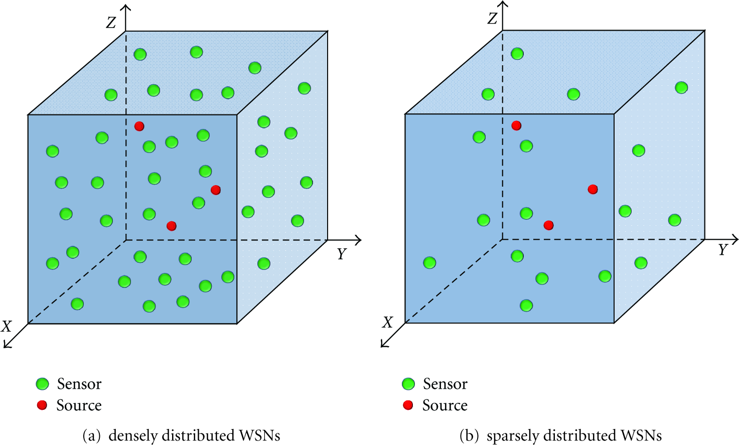
The geometry of WSNs and sources.

The positions of sources are relatively sparse in comparison with a large observation scene, which is shown in Figure 1. Here, the redundant dictionaries are adopted to represent the received signals of RSS-WSNs. The redundant dictionary is essentially the geometric projection in space. In the form of this dictionary, the measurement of mth node is denoted as

$s_m={\psi }_m\theta +w_m,$

(3)

where ${\psi }_m$ consists of a redundant dictionary. Other parameters are defined as follows:

$\begin{array}{c}{\psi }_m=\left(h_{m1},h_{m2},\dots ,h_{mN}\right),\\ h_{mn}=\frac{g_m}{{{\Vert {\vec{\mathbf{r}}}_m-{\vec{\mathbf{r}}}_n\Vert }_2}^{\alpha }},\\ \theta ={\left(0,p_1\dots p_k\dots 0\right)}^T,\end{array}$

(4)

where $m=\mathrm{1,2},\dots ,M,\mathrm{\hspace{0.17em}\hspace{0.17em}}n=1,2,\dots ,N$ , ${\psi }_m\in R^N$ , and $\theta \in R^N$ .

If the three-dimensional scene is divided into $N_x*N_y*N_z=N$   discrete subscenes, K sources are located in K subscenes. Ψ denotes the projection matrix from the nodes to the subscenes, which reflect the energy attenuation coefficients between the nodes and the subscenes in physics. The positions of the nonzero elements in θ are the positions of sources, the intensities of nonzero components are the power of the sources, and the number of nonzero components is the number of sources. Because K is much smaller than $N,\mathrm{\hspace{0.17em}\hspace{0.17em}}\theta$ is considered to be sparse. Thus, a sparse representation of received signal for single sensor is obtained.

One snap received signal is formulated in a matrix for RSS-WSNs with M nodes

$\begin{array}{cc}\hfill \left(\begin{array}{c}{s}_1\\ s_2\\ \mathrm{\hspace{0.17em}\hspace{0.17em}}⋮\\ s_M\end{array}\right)& =\left(\begin{array}{c}{\psi }_1\\ {\psi }_2\\ \mathrm{\hspace{0.17em}\hspace{0.17em}}⋮\\ {\psi }_M\end{array}\right)*\theta \mathrm{\hspace{0.17em}\hspace{0.17em}}+\left(\begin{array}{c}{w}_1\\ w_2\\ \mathrm{\hspace{0.17em}\hspace{0.17em}}⋮\\ w_M\end{array}\right)\hfill \\ \hfill & =\left(\begin{array}{cccccc}{h}_{11},& h_{12},& \dots & h_{1n}& \dots \mathrm{\hspace{0.17em}\hspace{0.17em}}& h_{1N}\\ h_{21},\mathrm{\hspace{0.17em}\hspace{0.17em}}\mathrm{\hspace{0.17em}\hspace{0.17em}}& h_{22},& \dots & h_{2n}& \dots & h_{2N}\\ ⋮& ⋮& \ddots & & \ddots & ⋮\\ h_{M1},\mathrm{\hspace{0.17em}\hspace{0.17em}}& h_{M2},& \dots & h_{1n}& \dots & h_{MN}\end{array}\right)*\theta \mathrm{\hspace{0.17em}\hspace{0.17em}}+\left(\begin{array}{c}{w}_1\\ w_2\\ \mathrm{\hspace{0.17em}\hspace{0.17em}}⋮\\ w_M\end{array}\right),\hfill \end{array}\mathrm{\hspace{0.17em}\hspace{0.17em}}$

(5)

where ${\psi }_m$ is defined as row vector of the redundant dictionary.

For simplicity, (5) can be written as

$S=\mathbf{\Psi }\theta +W,$

(6)

where $S=(s_1,s_2,\dots ,s_M),\mathrm{\hspace{0.17em}\hspace{0.17em}}S\in R^M$ , $\mathrm{\Psi }={({\psi }_1,{\psi }_2,\dots ,{\psi }_M)}^T,\mathrm{\Psi }\in R^{M*N}$ , and $W=(w_1,w_2,\dots ,w_M),\mathrm{\hspace{0.17em}\hspace{0.17em}}W\in R^N$ .

The advantage of this sparse representation is that signal   $\theta$ contains both the locations and the intensities of sources. Thus, the parametric estimation of the sources can be converted into the recovery of   $\theta$ . However, a large observation scene would mean that the length of θ is so long that the recovery is excessively complex.

2.2. CS-Based Sampling in RSS-WSNs

As mentioned above, S is expanded in redundant dictionary   $\mathrm{\Psi }$ , and the coefficient sequence θ is sparse. If Φ denotes WSNs' sampling mechanism, the measurement Z can be expressed as follows:

$Z=\mathit{\Phi }S+W_1=\mathit{\Phi }\mathit{\Psi }\theta +W_1,$

(7)

where $Z\in R^{N_S}$ , $\mathrm{\Phi }\in R^{N_S*M},\hspace{0.17em}{N}_S\le M$ , and $W_1=\mathrm{\Phi }W\in R^{N_S}$ .

Another important principle of CS theory is incoherent sampling. Incoherent sampling demands the coherence between sampling matrix (Φ) and representing matrix (Ψ) to be as small as possible. Usually, the coherence $\mu (\mathrm{\Phi },\mathrm{\Psi })$    between $\mathrm{\Phi }$   and   $\mathrm{\Psi }$ is defined as [25]

$\mu \left(\mathbf{\Phi },\mathbf{\Psi }\right)=\sqrt{N}\underset{1\le k\le N_S,1\le j\le N}{\max }\left|〈{\phi }_k,{\psi }_j〉\right|,$

(8)

where $\mathrm{\Phi }=[{\phi }_1,{\phi }_2,\dots ,{\phi }_{N_S}{]}^T$ ,   ${\phi }_k$    is row vector of Φ, and $\mathrm{\Psi }=[{\psi }_1,{\psi }_2,\dots ,{\psi }_N]$ , ${\psi }_j$   is column vector of $\mathrm{\Psi }·\mu (\mathrm{\Phi },\mathrm{\Psi })\in [1,\sqrt{N}]$ .

According to the measurement Z, ${\ell }_1,$   norm minimization can stably recover θ when the number of measurements exceeds [25]

$N_S\ge \text{C}\cdot {\mu }^2\left(\mathbf{\Phi },\mathbf{\Psi }\right)\cdot K\hspace{0.17em}\log \hspace{0.17em}N,$

(9)

where $N_S$ denotes the number of measurements and C is a known (small) constant which depends on the recovery precision.

If Ψ extends from an orthonormal basis to redundant dictionary, it is necessary to give restrictions to $\mathrm{\Phi }$      and   $\mathrm{\Psi }$ . A random sampling matrix needs to satisfy [23]

$P\left(\left|{\Vert \mathit{\Phi }v\Vert }_2^2-{\Vert v\Vert }_2^2\right|\ge \epsilon {\Vert v\Vert }_2^2\right)\le 2e^{-c{N}_s{\epsilon }^2/2}.$

(10)

Here, $v$    is any vector with the length of M, $\epsilon \in (\mathrm{0,1}/3)$ and $c>0$ . The intercoherence of   $\mathrm{\Psi }$ denotes $\mu (\mathrm{\Psi })={\max \hspace{0.17em}}_{1\le i,j\le N,i\ne j}\hspace{0.17em}|〈{\psi }_i,{\psi }_j〉|$ and ${\psi }_n\mathrm{\hspace{0.17em}\hspace{0.17em}}(n=1,2,\dots ,N)$ are the column vectors. When   $K-1\le 1/16\hspace{0.17em}{\mu }^{-1}$ , the   ${\ell }_1$   minimization can recover θ with a probability of at least $1-e^{-t}$ from the measurements, whose numbers satisfy [23]

$N_S\ge C_1\left(K\log \left(\frac{N}{K}\right)+C_2+t\right),$

(11)

where $C_1,\mathrm{\hspace{0.17em}\hspace{0.17em}}{C}_2,\mathrm{\hspace{0.17em}\hspace{0.17em}}t$   are constants that are related with the restricted isometry principle (RIP) of a sampling matrix.

In this study, the Bernoulli matrix is adopted as the sampling matrix that satisfies the restriction of (10). More details are shown in [23]. The variable of Bernoulli matrix ${\varphi }_{k,m}$ is shown as follows:

$\begin{array}{c}{\varphi }_{k,m}=\{\begin{array}{cc}1\mathrm{\hspace{0.17em}\hspace{0.17em}}\hfill & \text{with}\mathrm{\hspace{0.17em}\hspace{0.17em}}\text{probability}\mathrm{\hspace{0.17em}\hspace{0.17em}}0.5,\hfill \\ 0\mathrm{\hspace{0.17em}\hspace{0.17em}}\hfill & \text{with}\mathrm{\hspace{0.17em}\hspace{0.17em}}\text{probability}\mathrm{\hspace{0.17em}\hspace{0.17em}}0.5,\hfill \end{array}\\ \mathrm{\hspace{0.17em}\hspace{0.17em}}k=\mathrm{1,2},\dots ,N_s,\hspace{1em}m=\mathrm{1,2},\dots ,M,\hspace{1em}{N}_S\le M.\end{array}$

(12)

Φ consists of ${\varphi }_{k,m}$ , and the column vectors of Φ are irrelevant with each other. In physics, 0 and 1 mean that the nodes are disabled and enabled to receive the data, respectively. The number of rows in Φ is the sampling number   $N_S$ . Because this study focuses on the algorithm of source localization in sparse RSS-WSNs, the sampling number is assumed to be   $N_S=M$ , which means full samplings in space.

According to (9) and (11), θ can be recovered by minimizing   ${\ell }_0$ norm, which can be expressed in

$\widehat{\theta }=\arg \underset{\theta \in R^N}{\min }{\Vert \theta \Vert }_0,\mathrm{\hspace{0.17em}\hspace{0.17em}}\text{s}.\text{t}.\hspace{1em}{\Vert Z-\mathbf{\Phi }\mathbf{\Psi }\theta \Vert }_2\le \epsilon ,$

(13)

where ${\parallel \bullet \parallel }_0$ denote the ${\ell }_0$    norm.

Unfortunately, solving this ${\ell }_0$ minimization is a NP problem and imposes combinatorial complexity. Therefore, some simplifications are used. [8, 16] proposes solving ${\ell }_1$ minimization instead of ${\ell }_0$ minimization

$\widehat{\theta }=\arg \underset{\theta \in R^N}{\min }{\Vert \theta \Vert }_1,\mathrm{\hspace{0.17em}\hspace{0.17em}}\text{s}.\text{t}.\mathrm{\hspace{0.17em}\hspace{0.17em}}\hspace{1em}{\Vert Z-\mathbf{\Phi }\mathbf{\Psi }\theta \Vert }_2\le \epsilon .$

(14)

The optimization (14) is known as basis pursuit (BP). When the measurements contain noise, BP may be represented as the dual problem [8]

$\widehat{\theta }=\arg \underset{\theta \in R^N}{\min }\left({\Vert Z-\mathbf{\Phi }\mathbf{\Psi }\theta \Vert }_2+\lambda {\Vert \theta \Vert }_1\right),$

(15)

where ${\parallel \bullet \parallel }_1$ denotes the ${\ell }_1$   norm and λ is the coefficient that describes the tradeoff between denoising and retaining sparsity.

3. CS-Based Source Localization

3.1. Multiresolution Redundant Dictionary

A redundant dictionary is related to the grid number at each dimension ( $N_x,N_y,N_z$ ) and the dictionary arrangement. If   $N_x*N_y*N_z=N$ is assumed to be big, theoretical localization accuracy is increased, but the computation cost of signal recovery is extremely high. For a signal with the length of   $N$ , the optimization could be evaluated using $O(N)$ operations. If the optimization is divided into β steps, in which each recovery needs $\beta *O(N^{1/\beta })$ operations, such an approach could reduce the overall complexity of CS-based source localization from $O(N)$ to $\beta *O(N^{1/\beta })$ . Assuming   $N_x=N_y=N_z=1000$ ,   $\beta =3$ , the complexity would be reduced from $O(10^9)$ to $3$   *   $O(10^3)$ . Thus a multiresolution redundant dictionary is suitable for low-powered RSS-WSNs.

According to CS sample principle, θ could be stably recovered by ${\ell }_1$ norm minimization when the number of measurements must satisfy (11). Assuming $C=1$ and   $\mu (\mathrm{\Phi },\mathrm{\Psi })=0.75$ , the relationship between $N_S$ and the high bound of   $N$ for different K is shown in Figure 2. If the sample number is fixed, such as   $N_S=9$ , the length of θ must not exceed 25 for $K=5,\mathrm{\hspace{0.17em}\hspace{0.17em}}54$ for $K=4,\mathrm{\hspace{0.17em}\hspace{0.17em}}207$ for $K=3,\mathrm{\hspace{0.17em}\hspace{0.17em}}2980$ for $K=2$ , and $8.9\mathrm{\hspace{0.17em}\hspace{0.17em}}\times \mathrm{\hspace{0.17em}\hspace{0.17em}}10^6$ for $K=1$ . Too long θ would go against CS sample principle and lead to poor estimation for few spatial samples. Therefore, the multiresolution redundant dictionary could effectively control the length of θ to address this problem.

Figure 2

Relationship between sample number and the high bound of N.

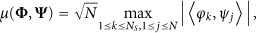
As mentioned above, a multiresolution redundant dictionary can sharply reduce the length of θ and the computation for a large-scale scene. Figure 3 shows the process of constructing a multiresolution dictionary. Firstly, the initial resolution is set to be low, and the sources are located in a certain grid or several grids by signal recovery. Secondly, the grid or the combination of several grids is considered as new space and is used to build a new redundant dictionary, which has smaller grids than before. Then sources are located in specified smaller grids by signal recovery. Thirdly, the combination of these smaller grids is considered as another new space, and the redundant dictionary is updated. Then the process is repeated until the minimum grid is up to resolution requirement.

Figure 3

Multiresolution redundant dictionary.

For the same scene, iterative times of recovery would decrease with the increasing of N when constructing a redundant dictionary. A bigger N is likely to disobey the CS sample principle. Therefore, it is necessary to ensure proper N to make a tradeoff between iterative times and incoherence and a tradeoff between iterative times and recovery precision.

3.2. Adaptive Dictionary Refinement

The spatial subdivision schemes of dictionary can be divided into uniform and adaptive ones. The length of each grid is equal for uniform schemes, while the length of each grid is weighted by the data-driven criteria for adaptive schemes. In this study, both schemes are adopted in the localization algorithm. Because of none prior source location, the initial dictionary is made up of uniform grids. Then sources may be located in one or several interested and coarse grids, which would be adaptively partitioned into many subgrids. The numbers of subgrids are weighted by the recovery signal ${\widehat{\theta }}^{\text{iter}-1}$ of previous iteration. There are   $N^{\text{iter}}(j)$ subgrids in jth interested grid, given by

$N^{\text{iter}}\left(j\right)=w^{\text{iter}}\left(j\right)*N,$

(16)

where N denotes the total number of subgrids in the current iteration. The weighted values $w^{\text{iter}}(j)$ can be calculated by the previous   ${\widehat{\theta }}^{\text{iter}-1}$ , expressed as

$w^{\text{iter}}\left(j\right)=\frac{{\widehat{\theta }}^{\text{iter}-1}\left(j\right)}{{\sum }_{j=1}^N{\widehat{\theta }}^{\text{iter}-1}\left(j\right)}.$

(17)

The elements of   ${\widehat{\theta }}^{\text{iter}-1}$   should be preprocessed by

$\mathrm{\hspace{0.17em}\hspace{0.17em}}{\widehat{\theta }}^{\text{iter}-1}\left(j\right)=\{\begin{array}{cc}{\widehat{\theta }}^{\text{iter}-1}\left(j\right),\hfill & {\widehat{\theta }}^{\text{iter}-1}\left(j\right)\ge 0,\hfill \\ 0,\hfill & \text{otherwise}.\hfill \end{array}$

(18)

Figure 4 shows the procedure of adaptive grid refinement in the iterations. First iteration adopts the uniform grid centers, and the sources are located coarsely in some grids (Figure 4(a)). Then these grids are split into subgrids with different resolutions depending on the estimated intensity from them. And the grid is more close to the source, which could have higher resolution, shown in Figures 4(b), 4(c), and 4(d).

Figure 4

Adaptive grid refinement in the iterations: the observation scene is 1000*1000*100.

3.3. Redundant Dictionary Arrangement

In this study, continuous coordinate indexing is utilized to arrange grids of redundant dictionary. The world Cartesian coordinates system is defined in Section 2.2. Additionally, we denote local axis as 1st-, 2nd-, and 3rd-axis depending on the indexing order, which are shown in Figure 5.

Figure 5

Continuous coordinate indexing of redundant dictionary in local coordinate system.

The indexing in local coordinate system has the following steps. Firstly, a 3rd-axis coordinate is fixed. Then the grids are arranged from small 1st-axis coordinate to big one on the plane that consists of 1st- and 2nd-axis, until all 2nd-axis coordinates are arranged. Secondly, turn to another plane that consists of 1st- and 2nd-axis. Then arrange all grids in this plane in the same manner as the first step. Finally, all 3rd-axis coordinates are arranged, and all grids are arranged (Figure 5). In other words, this redundant dictionary is indexed from 1st-axis to 2nd-axis, then to 3rd-axis. And the distance between neighbors in 1st, 2^nd, and 3rd-axis is 1, $N_{1\text{st-axis}}$ , and $N_{1\text{st-axis}}*N_{2\text{nd-axis}}$ , respectively. Note that $N_{1\text{st-axis}}$ , $N_{2\text{nd-axis}}$ , and $N_{3\text{rd-axis}}$ denote the number of grids in three axis, respectively.

After sensors are deployed randomly in the interest of scene, there are multiple sources to be located. The arrangement of a redundant dictionary impacts the capacity to resolve multiple sources. For the same three-dimensional scene, redundant dictionary could be indexed in six manners, called redundant dictionary arrangement (RDA), in the form of   $\kappa$ . RDA is essentially how to define 1st-, 2nd-, and 3rd-axis as X-, Y-, and Z-axis, respectively. There are six definitions shown in Figure 6. The distances between neighbors in X-, Y-, and Z-axis $(\mathrm{\Delta }{N}_{x(\kappa )}^{}$ , $\mathrm{\Delta }{N}_{y(\kappa )}^{}$ , $\mathrm{\Delta }{N}_{z(\kappa )}^{})$ under different RDAs are shown in Table 1.

Table 1

Six RDAs.

κ	Indexing order $1\text{st}\to 2\text{nd}\to 3\mathrm{rd}$	$\mathrm{\Delta }{N}_{x(\kappa )}^{}$	$\mathrm{\Delta }{N}_{y(\kappa )}^{}$	$\mathrm{\Delta }{N}_{z(\kappa )}^{}$
1	$Z\to Y\to X$	$N_y{N}_z$	$N_z$	1
2	$Y\to Z\to X$	$N_y{N}_z$	1	$N_y$
3	$X\to Z\to Y$	1	$N_x{N}_z$	$N_x$
4	$Z\to X\to Y$	$N_z$	$N_x{N}_z$	1
5	$Y\to X\to Z$	$N_y$	1	$N_x{N}_y$
6	$X\to Y\to Z$	1	$N_x$	$N_x{N}_y$

Figure 6

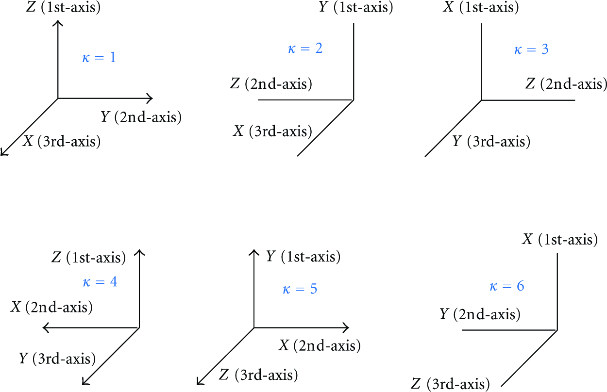
Six definitions of X-, Y-, and Z-axis.

Under certain form of RDA (κ), $\mathrm{\Delta }{N}_{\kappa }(k,j)$   denotes the distance between two arbitrary sources (k- and j-source) in   $\theta$ . (19) is used to calculate   $\mathrm{\Delta }{N}_{\kappa }(k,j)$

$\begin{array}{cc}\hfill \Delta N_{\kappa }\left(k,j\right)& =\left|\Delta N_{x\left(\kappa \right)}^{}{\left[\frac{\left(X_k-X_j\right)}{\Delta x}\right]}_I\right|\hfill \\ \hfill & \hspace{1em}+\left|\Delta N_{y\left(\kappa \right)}^{}{\left[\frac{\left(Y_k-Y_j\right)}{\Delta y}\right]}_I\right|\hfill \\ \hfill & \hspace{1em}+\left|\Delta N_{z\left(\kappa \right)}^{}{\left[\frac{\left(Z_k-Z_j\right)}{\Delta z}\right]}_I\right|,\hfill \end{array}$

(19)

where $(X_k,Y_k,Z_k)$ and $(X_j,Y_j,Z_j)$ are the positions of k- and j-source, respectively. $\mathrm{\Delta }x$ , $\mathrm{\Delta }y,$   and $\mathrm{\Delta }z$ is the grid unit of $X\text{-}$ , $Y\text{-}$ , and $Z\text{-}$ axis, respectively, and $[A{]}_I$ denotes the nearest integers less than or equal to   $A$ .

The optimization of RDA is essentially how to refine the direction of X-, Y-, and Z-axis in order to make the distance of two close sources in θ as large as possible, which is shown in

$\widehat{\kappa }=\arg \underset{\kappa }{\max }\left\{\underset{1\le k\ne j\le K}{\min }\left[\Delta N_{\kappa }\left(k,j\right)\right]\right\},$

(20)

where   ${\min \hspace{0.17em}}_{1\le k\ne j\le K}\mathrm{\hspace{0.17em}\hspace{0.17em}}[\mathrm{\Delta }{N}_{\kappa }(k,j)]$ is the minimal distance of K sources.

For instance two isotropic acoustic sources have been coarsely estimated and found that their distance has one grid in X-axis after previous iteration. This means that ${[(X_1-X_2)/\mathrm{\Delta }x]}_I=1$ and $Y_1=Y_2,\mathrm{\hspace{0.17em}\hspace{0.17em}}{Z}_1=Z_2$ . If $\kappa =3,\mathrm{\hspace{0.17em}\hspace{0.17em}}6,\mathrm{\hspace{0.17em}\hspace{0.17em}}\mathrm{\hspace{0.17em}\hspace{0.17em}}\mathrm{\Delta }N=1;$   if $\kappa =4,\mathrm{\hspace{0.17em}\hspace{0.17em}}5,\mathrm{\hspace{0.17em}\hspace{0.17em}}\mathrm{\Delta }N=N_z$   or   $N_y$ ; if $\kappa =1,\mathrm{\hspace{0.17em}\hspace{0.17em}}2,\mathrm{\hspace{0.17em}\hspace{0.17em}}\mathrm{\Delta }N=N_y\mathrm{\hspace{0.17em}\hspace{0.17em}}{N}_z$ . Figure 7 shows the relative positions of these two sources under different RDAs. Theoretically speaking, it is more accurate to recover the signal whose nonzero components distance is $N_y\mathrm{\hspace{0.17em}\hspace{0.17em}}{N}_z$ than the signal whose nonzero components distance is 1, especially when this signal is sparse in the form of a redundant dictionary. Accordingly, the optimization of RDA can improve the ability to distinguish close sources.

Figure 7

Two sources are located in θ.

3.4. Signal Recovery Algorithm

It is well known that the signal can be recovered by nonconvex optimization, convex optimization, and statistics optimization. Orthogonal matching pursuit (OMP) [6] is a typical nonconvex optimization, which has a high calculation efficiency. And least absolute shrinkage and selection operator (LASSO) [7] is a typical convex method, that has a high recovery accuracy but the calculation is more complex than OMP. Statistics optimization, such as sparse Bayesian learning [26], has a higher calculation efficiency than convex algorithm and a higher recovery accuracy than nonconvex algorithm. Accordingly, sparse Bayesian learning [26] is utilized to locate sources.

In sparse Bayesian learning, a three-stage hierarchical form of Laplace priors is utilized to model the sparsity of the unknown signal   $\theta$ , and the solving of (14) or (15) is done by maximizing posterior probability. θ is assumed to satisfy the following equation:

$p\left(\theta \hspace{0.17em}|\hspace{0.17em}{\lambda }_L\right)=\frac{{{\lambda }_L}^{N/2}}{2^N}\exp \left(-\sqrt{{\lambda }_L}{\Vert \theta \Vert }_1\right),$

(21)

where ${\lambda }_L$   is the coefficient of Laplace priors. The Laplace priors mean that θ submits to Gauss distribution, whose mean is zero and variance follows the Gamma distribution. ${\lambda }_L$ is essentially the coefficient of Gamma distribution, which impacts $p(\theta |{\lambda }_L)$ and recovery accuracy.

3.5. CS-Based Source Localization Procedure

The proposed CS-based source localization algorithm is summarized in Algorithm 1.

Algorithm 1: CS-based source localization algorithm.

Input: The positions of randomly deployed sensors and their measurements Z.

Initialization: Construct the sampling matrix   $\mathrm{\Phi }$ . The initial search space is the three-dimensional scene covered by RSS-WSNs. The RDA κ is arbitrary. $\mathit{\theta }=\mathit{0}$ , the set of nonzero elements in θ is null, and the iterative times is zero.

Step $\mathit{1}$ : The process of estimation: $\mathbf{i}\mathbf{t}\mathbf{e}\mathbf{r}\leftarrow \mathbf{i}\mathbf{t}\mathbf{e}\mathbf{r}+\mathbf{1}$ .

(a) Construct redundant dictionary depending on the search space.

(b) ${\widehat{\theta }}^{\text{iter}}=\arg {\min \hspace{0.17em}}_{\theta \in R^N}\hspace{0.17em}({\parallel Z-\mathrm{\Phi }\mathrm{\Psi }\theta \parallel }_2+\lambda {\parallel \theta \parallel }_1)$ . (More details in Section 3.4.)

  ${\widehat{\theta }}^{\text{iter}}(j)=\{\begin{array}{cc}{\widehat{\theta }}^{\text{iter}}(j),& {\widehat{\theta }}^{\text{iter}}(j)\ge \tau \ge 0,\\ 0,& \text{otherwise},\end{array}$ τ is the threshold to determine whether an element is a nonzero element.

(c) Adaptive dictionary refinement based on   $w^{\text{iter}+1}(j)={\widehat{\theta }}^{\text{iter}}(j)/{\sum }_{j=1}^N{\widehat{\theta }}^{\text{iter}}(j)$ .

  ${\mathrm{\Lambda }}^{\text{iter}}=\{j\mathrm{\hspace{0.17em}\hspace{0.17em}}|{\widehat{\theta }}^{\text{iter}}(j)>\tau \}$ ,   $K={\parallel {\mathrm{\Lambda }}^{\text{iter}}\parallel }_0$ . Select the center of the grid ${{\mathrm{\Lambda }}_k}^{\text{iter}}$   as the source positions   ${\overrightarrow{\widehat{\mathbf{r}}}}_k^{}{\hspace{0.17em}}^{\text{iter}},\mathrm{\hspace{0.17em}\hspace{0.17em}}\mathrm{\hspace{0.17em}\hspace{0.17em}}k=\mathrm{1,2},\dots ,K$ . (More details in Section 3.2.)

(d) If $K=1$ , RDA is unchanged.

If   $K>1$ , optimize RDA for the next iteration. $\widehat{\kappa }=\arg {\max \hspace{0.17em}}_{\kappa }\hspace{0.17em}\{{\min \hspace{0.17em}}_{1\le k\ne j\le K}[\mathrm{\Delta }{N}_{\kappa }(k,j)]\}$ . (More details in Section 3.3.)

Step $\mathit{2}$ : Output ${\overrightarrow{\widehat{\mathbf{r}}}}_k^{}{\hspace{0.17em}}^{\text{iter}}$   until the resolution is up to initial setting.

4. Simulations and Analysis

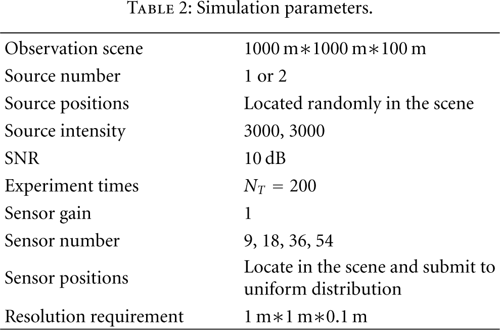
In order to evaluate the performance of the proposed algorithms, we conducted some typical numerical simulations. The simulation parameters are set in Table 2.

Table 2

Simulation parameters.

Observation scene	1000 m*1000 m*100 m
Source number	1 or 2
Source positions	Located randomly in the scene
Source intensity	3000, 3000
SNR	10 dB
Experiment times	$N_T=200$
Sensor gain	1
Sensor number	9, 18, 36, 54
Sensor positions	Locate in the scene and submit to uniform distribution
Resolution requirement	1 m*1 m*0.1 m

4.1. RSS-WSNs Deployment

Generally speaking, sensor nodes can be deployed in a plane, or in two planes, or in a three-dimensional space. The manner of deployment [27] is classified into random distribution and uniform formation. In this study, area coverage is the primary objective for deployment, and more details are in paper [7, 13, 28]. For different localization algorithms, it is necessary to deploy nodes in a proper manner to improve localization accuracy. For ML, the more uniform the nodes are within the sensor field layout, the smaller the CRLR and the higher the localization accuracy are.

The localization accuracy is defined as the root mean square (RMS), given by

$\text{RMS}=\frac{1}{N_T}\sqrt{{\displaystyle \sum }_{i=1}^{N_T}{\Vert {\overrightarrow{\widehat{\mathbf{r}}}}_i-{\vec{\mathbf{r}}}_{i0}\Vert }_2^2}.$

(22)

Here, ${\vec{\mathbf{r}}}_{i0}$ is the source position, ${\overrightarrow{\widehat{\mathbf{r}}}}_i$ is the estimated position in i-experiment, and $N_T$ is the experiment time.

However, the CS-based algorithm is the opposite of ML. Because the distribution of nodes impacts on   $\mu (\mathrm{\Phi },\mathrm{\Psi })$ , the proper RSS-WSNs' deployment can make Φ to be as incoherent with   $\mathrm{\Psi }$ as possible. The more randomly the nodes are deployed, the smaller $\mu (\mathrm{\Phi },\mathrm{\Psi })$   and RMS are.

We contract the impacts on   $\mu (\mathrm{\Phi },\mathrm{\Psi })$ and RMS from the four RSS-WSNs' deployments, which are in uniform formation in a plane, uniform formation in two planes, random distribution in a plane, and random distribution in two planes, respectively. The simulation results are presented in Figure 8. Figures 8(a) and 8(b) show the deployment impacts on RMS, and Figures 8(c) and 8(d) show the deployment impacts on $\mu (\mathrm{\Phi },\mathrm{\Psi })$ . The triangles and the squares represent uniform formation and random distribution, respectively.

Figure 8

RSS-WSNs' deployment impacts RMS and $\mu (\mathrm{\Phi },\mathrm{\Psi })$ .

In Figures 8(a) and 8(b), the RMS of random distribution is smaller than the RMS of uniform formation, especially when $N_S$   is 9 and 18. It is because that $\mu (\mathrm{\Phi },\mathrm{\Psi })$ of random distribution is smaller than $\mu (\mathrm{\Phi },\mathrm{\Psi })$ of uniform formation, which is shown in Figures 8(c) and 8(d). Reducing $\mu (\mathrm{\Phi },\mathrm{\Psi })$ can weaken the coherence between $\mathrm{\Phi }$   and Ψ, which is good for signal recovery. Simulations demonstrate that the random deployment of RSS-WSNs can weaken the coherence between Φ and Ψ, hence reducing the RMS.

4.2. Coefficients of the Recovery Algorithm

As mentioned above, ${\lambda }_L$   determines   $p(\theta \hspace{0.17em}|\hspace{0.17em}{\lambda }_L)$ . Consequently, it impacts the RMS of source localization. $p(\theta \hspace{0.17em}|\hspace{0.17em}{\lambda }_L)$   is a function of   $K$   and   ${\lambda }_L$ which is shown in Figure 9(a). When ${\lambda }_L$   ranges among 0.1, 1, 5, 10, and 20. And RMS varies as   $N_S$   and ${\lambda }_L$ change, which is shown in Figure 9(b).

Figure 9

Coefficients for recovery algorithm.

For the same   $K$ , $p(\theta \hspace{0.17em}|\hspace{0.17em}{\lambda }_L)$ increases as ${\lambda }_L$ decreases. It means that the probability that $\theta$    has K-sparsity increases. For the same   $p(\theta \hspace{0.17em}|\hspace{0.17em}{\lambda }_L)$ , K increases as ${\lambda }_L$ decreases (Figure 9(a)). If ${\lambda }_L$ is extremely small, the probability that θ has a big K is large, which would lead to the appearance of fake sources. Because of this relationship between $p(\theta \hspace{0.17em}|\hspace{0.17em}{\lambda }_L)$ and   ${\lambda }_L$ , RMS is always below 1 m when ${\lambda }_L=0.1$   (as shown in Figure 9(b)). After comprehensive consideration of RMS and false alarms, the coefficient is chosen to   ${\lambda }_L=0.1$ .

4.3. Single Source Localization

In this subsection, the sample number $N_S$ ranges from 9, 18, 36 to 54,and the nodes are randomly deployed in a three-dimensional observation scene. RMS is related with SNR and $N_S$ , which is shown in Figure 10. The blue squares denote $N_S=9$ , the red upward-pointing triangles $N_S=18$ , the green circles $N_S=36$ , and the black downward-pointing triangles $N_S=54$ .

Figure 10

RMS varies with SNR (single source).

Figure 10 shows that higher SNR leads to lower RMS for the same   $N_S$ , and more samples (or bigger   $N_S$ ) leads to lower RMS for the same SNR. Especially when SNR = 10 dB and the sample number is above 18, RMS is below 3 m. As SNR increases, RMS decreases until below 1 m. When   $\text{SNR}\ge 20\hspace{0.17em}\text{dB}$ , the decreasing of RMS becomes slower along as $N_S$   increases. When $\text{SNR}\ge 20\hspace{0.17em}\text{dB}$ , $N_S=9$ makes RMS below 1 m.

In order to compare with other existing methods, the alternating projection (AP) algorithm [9] is also simulated as one effective localization algorithm based on ML. AP utilizes matrix projection to replace the inversion of matrix, and it locates unknown multiple sources through alternating optimization. The simulation results are shown in Figure 11 and Figure 13.

Figure 11

Compared to AP (single source).

For the same   $N_S$ , CS-based localization algorithm has lower RMS than AP. We found that the performance of CS-based algorithm when $N_S=18$ is similar to or better than the performance of AP even when $N_S=36$ . For instance, as SNR = 0 dB or 10 dB, RMS of CS-based ( $N_S=18$ ) is similar to AP ( $N_S=36$ ), but as   $\text{SNR}\ge 20\hspace{0.17em}\text{dB}$ , RMS of CS-based ( $N_S=18$ ) is smaller than AP ( $N_S=36$ ). The same situation happens between CS-based when $N_S=9$ and AP when   $N_S=18$ . As SNR = 0 dB or 10 dB, CS-based is similar to AP, but as   $\text{SNR}\ge 20\hspace{0.17em}\text{dB}$ CS-based is better than AP. Thus CS-based algorithm needs smaller nodes than AP algorithm to achieve the same RMS. When RSS-WSNs are sparsely distributed, CS-based performance is better than AP.

4.4. Two-Source Localization

The observation scene can be adaptively divided into subscenes through constructing redundant dictionaries. For multiple sources, their locations can be converted into estimating of the positions of one source or two closely sources in a subscene. As mentioned above, single-source localization has been analyzed. It is known that RMS of multiple sources is a function of SNR, $N_S$ , and the distance between two sources. We assume SNR to be 20, 10, 0, and −10 dB, $N_S$ to be 36 and 18, and the distance between two sources to be 1 m, 5 m, and 25 m, respectively. The histograms of the estimated number of sources at different SNR and source distances are shown in Figure 12.

Figure 12

Distribution of the estimated number of sources of different SNR and $N_S$ (two sources).

Figure 13

Contrast between CS-based and AP in localization performance (two sources).

When SNR is 20 or 10 dB (Figures 12(a), 12(b), 12(e), and 12(f)), RSS-WSNs can stably distinguish two sources with the probability above 0.8, even if the distance of two sources is close to the resolution requirement (1 m). The probability of distinguishing sources decreases as SNR decreases. Especially, if SNR = −10 dB, the probability that two sources are well separated is below 0.5 (Figure 12(d)). Comparing Figures 12(a)   12(b) to 12(e)   12(f), it is found that few spatial samples would make the probability of fake source greater. For example, as SNR = 10 dB and $N_S=18$ , the probability of fake source is nearly up to 0.2. Additionally, Figure 12 shows that the probability of accurate estimation increases with the increasing of the distance between sources.

We explore the RMS of CS-based and AP algorithm in locating two sources, especially when they are close to each other. SNR is assumed to be 20 dB, and the distance between two sources ranges from 1 m to 29 m, increasing in steps of 4 m. The contrast between CS-based and AP is illustrated in Figure 13. The dotted lines and the solid lines stand for AP and CS-based, respectively. The triangles and the squares are the first source and the second one, respectively.

In Figure 13, for CS-based and AP algorithm, simulation shows that the RMS of locating two sources is larger than that of locating a single source. It is because the parameters that are needed to estimate increase with the augment of the number of sources. In CS-based algorithm, the augment of source number results in the augment of the sparsity   $K$ . If $N_S$ is fixed, the augment of K would lead to the decreasing of location accuracy.

Theoretically, RMS decreases as the distance between sources increases for both CS-based and AP. However, when nodes are sparse, the RMS of multiple sources using AP is around 15 m (Figure 13). It is because the performance of AP has a strong relationship with the density of nodes, and RMS decreases as the density of nodes increases up to a certain level. If the density is not up to this level, RMS does not obviously decrease with the great increasing of the distance. However, CS-based algorithm has a different performance. At the same condition, the RMS of CS-based is smaller than AP, especially when    $N_S=9$   or 18.

In Figures 13(c) and 13(d), when the two sources are close to each other   $(d\le 13\hspace{0.17em}\text{m})$ , RMS does not decrease as $N_S$ increases from 36 to 54. This is because their positions of them in θ are too close to precisely recover   $\theta$ . Thus, it is necessary to optimize RDA (shown in (20)) to resolve two close sources.

In order to explore the impact from the optimization of RDA, two sets of simulation results are shown in Figure 14. One set is without RDA optimization (dashed line), and the other is with RDA optimization (solid line). The triangles and the squares represent the first source and the second source, respectively.

Figure 14

RDA impacts on RMS.

In Figure 14, CS-based localization algorithm improves with RDA optimization. The RMS of two sources with the procedure is smaller than that without the procedure, which is obvious when the distance between the sources is less than 21 m. This demonstrates that RDA optimization can effectively improve the capacity to resolve multiple close sources. However, when two sources are far apart (i.e., the distance between the sources is more than 21 m), the impact on RMS from the procedure is little. This is because no matter which RDAs are utilized, the distance between sources is enough to be resolved. At this time, RDA optimization is not of much importance.

5. Conclusions and Outlook

This work proposes an effective source localization algorithm based on CS, which is used on sparsely distributed RSS-WSNs. Extensive simulations show that the proposed algorithm consistently outperforms the existing ML algorithms. Compared to ML, CS-based algorithm improves the accuracy of single- and multiple-sources localization at the same number of samples. With the same accuracy of localization, this algorithm can effectively reduce the number of spatial samples.

Additionally, multi-resolution redundant dictionary reduces the complexity of calculation, and the adaptive dictionary refinement and the optimization of RDA can improve the efficiency of multiple source localization. A simulation demonstrates that the random deployment of nodes is more suitable to this algorithm than uniform formation.

There are other adaptive spatial partitioning approaches to construct redundant dictionary, such as KD tree or RP tree. Future work concerns about tree partitioning and treeindexing in CS-based source location algorithm.