
Abstract
We use molecular dynamics to simulate fluid flows between two parallel plates with constant wall temperature. Unlike the usual approach in molecular dynamics, instead of applying an external force on the molecules, the periodic boundary conditions are modified to create a pressure difference between the inlet and the outlet sections of the computational domain. The simulation results include velocity, pressure, density, and temperature profiles obtained by the new method. These results are compared with approximate solutions for nonisothermal Poiseuille flows. The method is also applied to simulate a flow in a rib-roughened channel.
1. Introduction
Over the past decades, nano/microfluidic systems have seen a rapid development and contribute to a revolution in many areas such as biotechnology and medicines. At the same time, calculation methods are also needed to analyze the reliability of the systems. The main challenge of the nano/microfluidics computations is that the studied system has a considerable surface/volume ratio so that the surface phenomena become highly important. These size effects cannot be solved by the traditional computational method for fluid dynamics.
Depending on the nature of the problem, there are different suitable computational methods, such as those based on the Navier-Stokes and energy equations, the Burnett or super-Burnett models [1–3], and the direct simulation Monte Carlo methods [4]. For nanoflows, the molecular dynamics (MD) method is one of the most accurate methods since realistic interactions between particles or between particles and boundaries may be accounted for.
One of the fundamental and practical problems in fluid mechanics is the steady-state flow between two parallel plates, the plane Poiseuille flow. Under the incompressibility assumption, the problem has a straightforward analytical solution. It is also studied extensively by other methods (Karniadakis et al. [5]). Most of the molecular dynamic simulations reported in the literature ([6–9], e.g.) concern flows driven by acceleration body force, rather than pressure driven flow. These limitations are due to the usage of the periodic boundary conditions which cannot generate pressure gradient inside the simulation domain. Several authors (Lupkowski and Van Swol [10], Li et al. [11], and Sun and Ebner [12]) have developed new techniques to mimic flows induced by pressure difference. Lupkowski and Van Swol [10] placed two rigid walls at the inlet and outlet and applied external forces on them. Li et al. [11] used a fictitious membrane which allows atoms to pass from one direction and forces atoms from the other direction to be elastically reflected with a given probability. Sun and Ebner [12] simulated 2D fluid flows in a long box while controlling the temperature at the two ends.
The present paper aims at presenting a new molecular dynamics approach based on pressure differences. Section 2 gives the problem statement and presents some approximate analytical solutions reported in the archival literature for Poiseuille flows. The pressure expression and the pressure difference from the atomistic point of view are also discussed. Section 3 is focused on the implementation of periodic boundary conditions linked to the pressure difference concept and its implementation in an MD code. The results of simulations are then compared with approximate analytical solutions of the Navier-Stokes and energy equations in Section 4. The application of the present method to fluids other than ideal gases and to rib-roughened channels is also discussed. Finally, some conclusions and perspectives are given in Section 5.
2. Problem Description and Theoretical Background
2.1. Problem Description
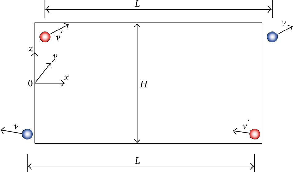
The objective of the present work is to study the fluid flows through a nanochannel. In the cartesian coordinate system
The Knudsen number, Kn, is a quantity to identify the fluid flow regime: from continuum (small Kn) to molecular flow regime (high Kn). The range of Kn chosen in the present study,

where λ is the mean free path, and H is a characteristic scale of the channel. In this work, λ is estimated by

The quantities n and σ in (2) are the density number and the diameter of the fluid molecules, respectively. For Lennard Jones (LJ) fluids, the molecular diameter value σ is approximately taken equal to the σ parameter appearing in the LJ potential formula introduced in Section 4.1.
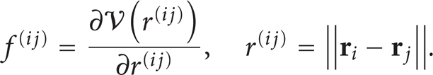
In what follows, the terms “pressure-driven flow” and “acceleration-driven flow” are employed to define two particular cases: (i) the body force ργ applied on a unit fluid volume is zero, and the pressure p decreases along the flow direction,

where a2 is a positive dimensionless constant related to pressure gradient (or body force), viscosity, slip length, and so forth. It is noted that (3) is generally obtained for incompressible fluids, but it is also valid for compressible fluid flows in a long channel [13]. In the latter case, v and a2 are functions of the streamwise coordinate x.
An approximation solution of the energy equation can be obtained by neglecting the convective term [14]. The temperature T becomes then a quartic function of the coordinate z,

Equation (4) is based on the incompressibility assumption. For compressible fluid flows in a long channel, Cai et al. [15] used a perturbation technique to derive the following temperature distribution:

The dimensionless coefficients

In Section 4, MD simulations are used to reexamine the validity of the velocity and temperature profiles given by (3)–(6) and to determine the coefficients a i , b i , c i , and d i by curve fitting.
2.2. Pressure Tensor and Pressure Difference
Before proceeding the molecular dynamics simulation, let us look at the definition of pressure tensor from the atomistic point of view. Using statistical mechanic theory, Irving and Kirkwood [16] derived the following pressure tensor decomposition (IK):

The kinetic term

The term inside the angular bracket
In (8), the notation

Equations (10) and (8) show that the derivation of IK pressure tensor involves an infinite sum of high-order derivatives of the delta function and ensemble average, not suitable for MD computations. A more convenient form of the pressure tensor and an associated calculation method, the method of plane (MOP), was proposed by Todd et al. [17] and by Evans and Morriss [18]. When the fluid density is uniform, the operator O i,j is reduced to unity, and (8) becomes (see [17, 19–22])
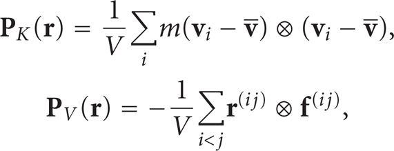
where V is the volume of the fluid element located at
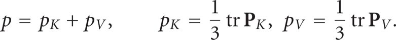
It is clear that for low-density fluids, high temperature, and small interaction energy ∊, the pressure is reduced to the kinetic part p K , as for ideal gases. For the other fluids, the potential part p V cannot be neglected. The pressure difference Δp between two points at distance Δl reads

The pressure components P
x,x
, P
y,y
, P
z,z
, number density n, and stream velocity

As it will be discussed in the following, all these conditions are satisfied in our MD simulation algorithm if we apply periodicity for the boundary conditions in the y direction. However, n, p, and T can all vary in the flow direction x. We note that in the steady-state regime, all quantities like T, p, p
V
, and n are stable with time, and thus their differences

If the stream velocity is much smaller than the thermal velocity, we can obtain a simplified expression for the temperature difference as
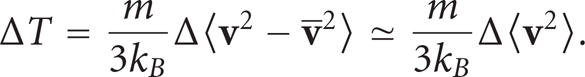
The objective of the MD method discussed in what follows is to maintain the differences in squared velocity and, thus in temperature, in direction x. By that way, we can indirectly generate the pressure difference Δp. In the case where density ρ is invariant in x-direction (incompressible flow assumption), the temperature difference is proportional, for an ideal gas, to the pressure difference since

3. Numerical Procedure
In molecular dynamics, periodic boundary conditions (PBC) applied to velocities are powerful techniques to reduce the study of a large system to a smaller one far from the edge. Considering a simulation domain as a cube, PBC requires that if a molecule passes through one face, it reappears on the opposite face with the same velocity. Obviously, there is no difference in pressure, density, or temperature between any two opposite faces of the simulation domain. Consequently
3.1. Modified Periodical Boundary Conditions
In our problem, all the virial pressure components P
x,x
, P
y,y
, and P
z,z
do not vary along y, which can be satisfied by the traditional PBC applied on the faces
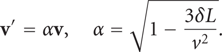
Usually, to keep unchanged the total number of molecules in the domain whenever a molecule goes out of the domain, we must insert another molecule inside. Thus, if we relax the PBC constraints, there are many ways to assign velocities to ingoing molecules, either independent of or dependent on the outgoing ones. In this paper, we generalize the PBC to account for the pressure difference by maintaining the difference in squared velocity at the two opposite faces × = 0 and
From (15) and (16), we know that a constant pressure difference is related to a constant difference in squared velocity. A constant parameter δ is thus used to create a constant difference in squared velocity between the inlet and outlet faces (see Figure 1). In order to apply a velocity square difference equal to a constant

Analogously, if a molecule crosses the face × = 0 with a velocity
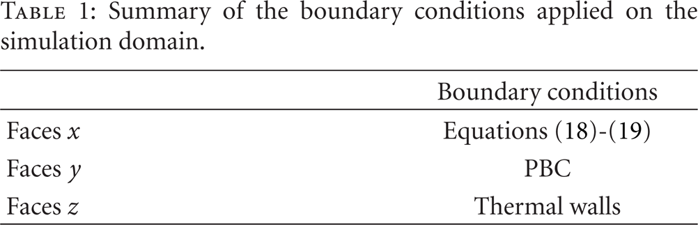
Since
Summary of the boundary conditions applied on the simulation domain.
4. Results
4.1. Molecular Dynamic Simulations of Ideal Gas Flows
To model the interaction between the molecules, the 6–12 Lennard Jones potential is used

where ∊ is the depth of the potential well, σ is the finite distance at which the interparticle potential is zero, and r is the distance between the particles.
The potential well depth parameter is
Input data for the first series of MD simulations.
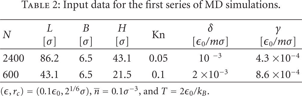
The two walls are modeled as thermally diffusive walls at the same and constant temperature. Whenever a molecule arrives at a wall, it is reflected with the velocity corresponding to the wall temperature
In our simulations, the global number density

nbin being the particle number in the bin. The local pressure

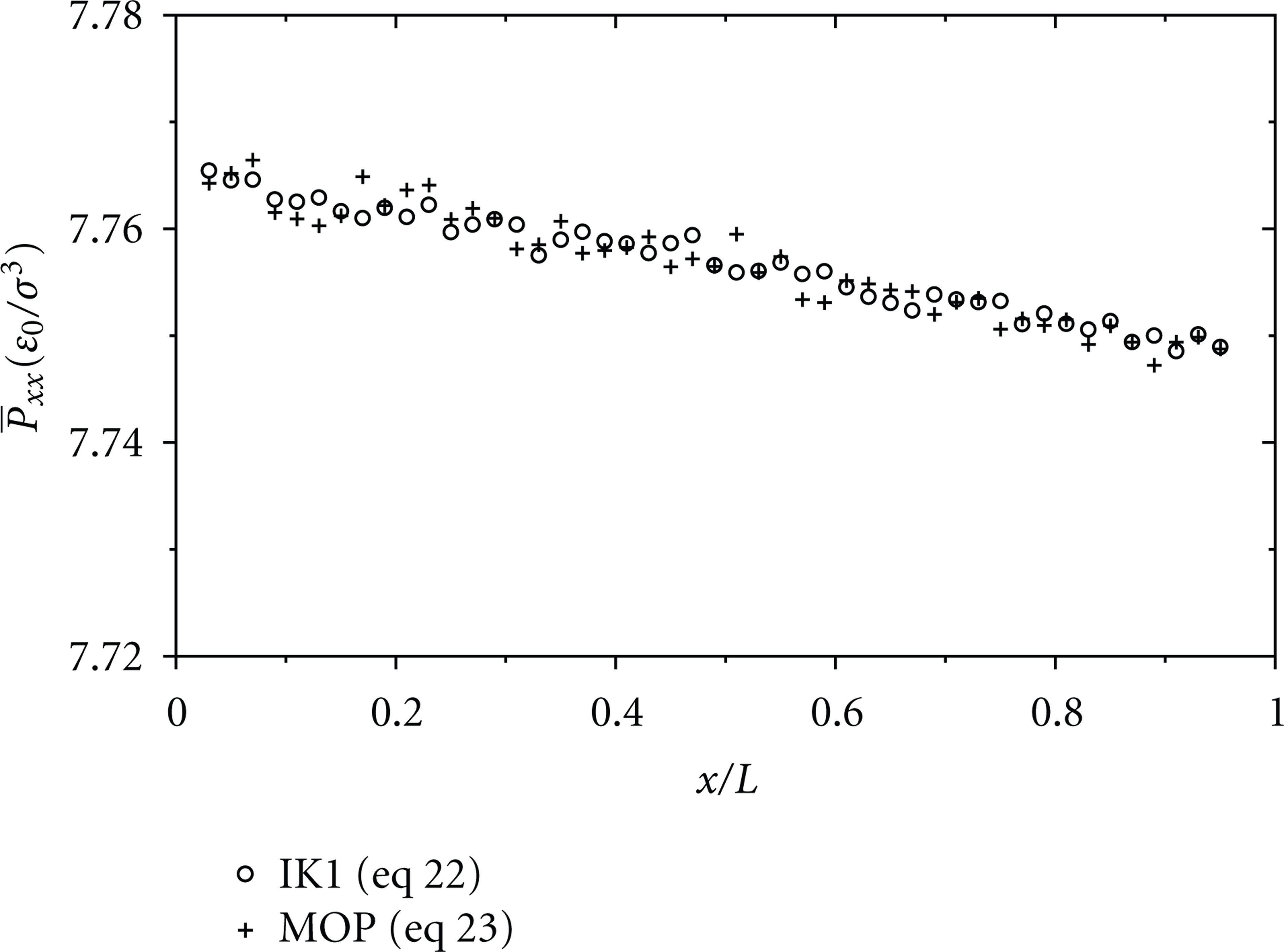
The pressure components were also computed by using the method of plane [17, 26]. With α, β being x, y, or z, the pressure component P β,α along direction β and acting on the area element A α normal to the axis α is defined by
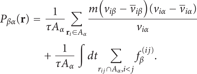
In (23), the first sum is for all molecules crossing the area element A α over the period τ, and the second sum is for all pairs whose distance vectors cut the area element A α . The temperature T of one bin is then calculated by

In what follows, the x-distributions of pressure, temperature, and density correspond to an average on y and z of the local quantities
Pressure distribution (

Distribution of pressure
From the simulations, the axial pressure distribution is plotted in Figure 2 for the pressure-driven and the acceleration-driven flows with
In order to know how the pressure difference is distributed in the x-, y-, z-directions, the pressure components


Dimensionless density profile (
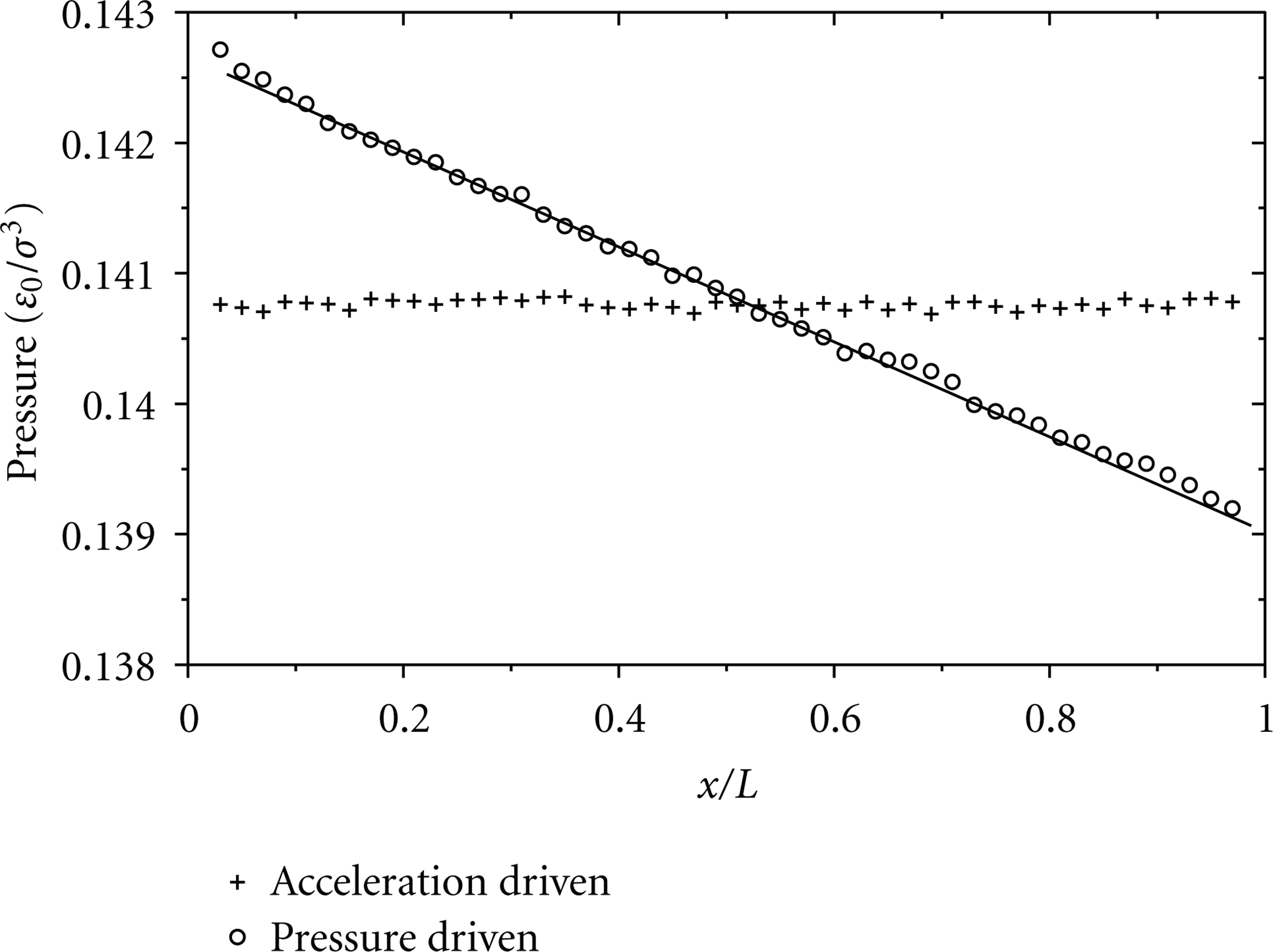
Figure 6 shows that acceleration and pressure-driven flows exhibit parabola-like velocity profiles in the center region of the channel, in agreement with (3). Near the wall where the Knudsen layer dominates, the velocity distribution tends to deviate from the solution given by (3), and a velocity slip at the wall is predicted. Based on the kinetic theories, different models have been derived to explain the slippage [5], and generally, the slip effect becomes important when the Knudsen number increases. The little difference in velocity profile between the two types of flow shows that, despite their different microscopic natures, volume forces can be seen as equivalent to pressure gradients at the macroscopic scale.
Dimensionless velocity profile in half of the channel cross-section for Kn = 0.05 and Kn = 0.1 (
About the temperature profile across the channel width, there is no visible difference between acceleration and pressure-driven formulations whatever Kn (Figure 7). The temperature profile cannot be fitted by any of the three approximate analytical solutions ((4)–(6)). The temperature is minimal at the center of the channel and increases rapidly near the wall, which does not agree with the approximate solutions obtained with the incompressible assumption ((4)-(5)). With the simulation conditions reported in Table 2, this reverse trend cannot thus be explained by using the incompressible flow equations. This anomaly was also observed by using DSMC method [27] and super-Burnett (SB) method [28]. Note that the flow speeds in our simulations are very small, as in [27, 28].

Dimensionless temperature profile (
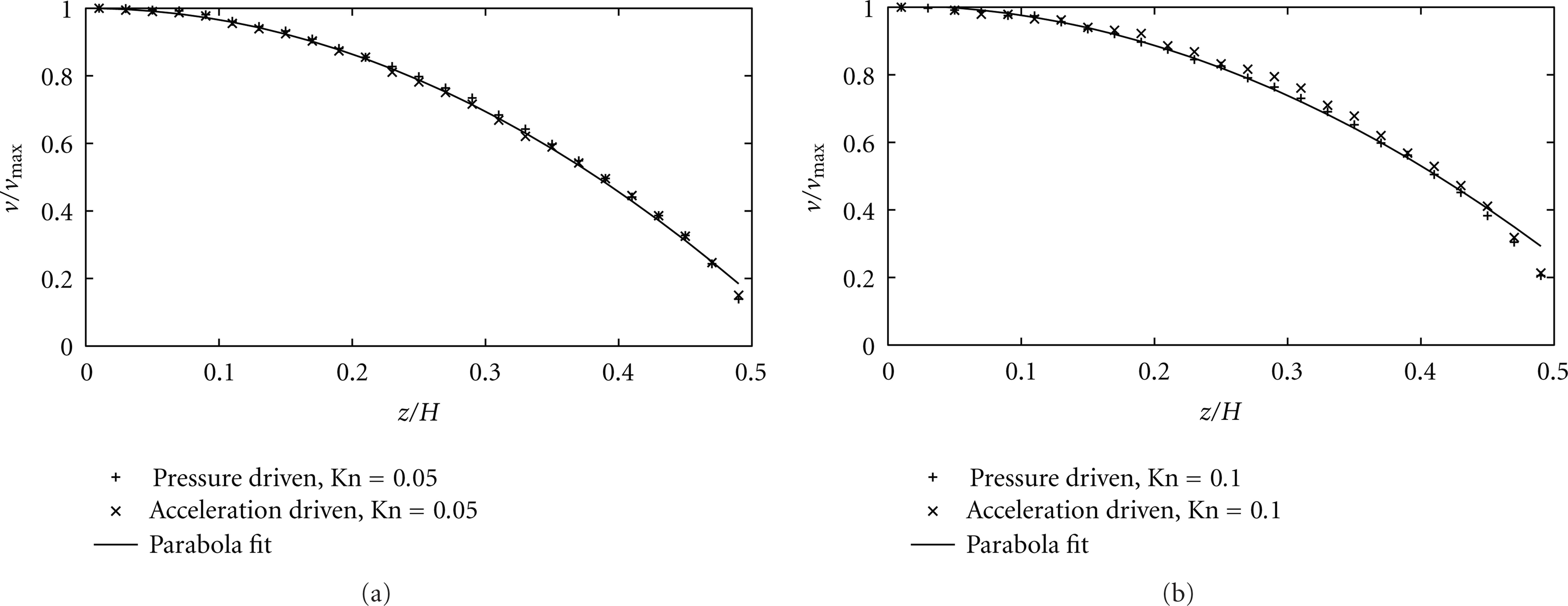
Next, we study the influence of γ and δ on the temperature profile. By increasing the acceleration parameter γ or the δ-parameter (squared velocity), the stream velocity is increased. A change in the form of the temperature profile is observed in Figures 8 and 9 as γ (or δ) increases. At high values of γ (or δ), the temperature profiles seem to be closer to the approximate solutions which predict a maximum at the center of the channel and a minimum at the walls. At small values of γ (or δ), the temperature profiles for the two flow types differ just a little. However, at high values of γ (or δ), the discrepancy becomes more important: the curvature at the center of channel for the pressure-driven flow case is higher than that for the acceleration-driven flow case. Using a curve-fitting procedure, we find that the temperature profile of the pressure-driven flow case agrees quite well with the quartic expression (5). The temperature for the acceleration-driven flow case does not fit well with (4). To explain this discrepancy, Todd and Evans [6] argued that the transport coefficients are not constant and that an additional cross-coupling between strain rate and heat flux exists. They proposed a correction to (5) with a
Variation of temperature profile when increasing the pressure gradient or parameter δ (Kn = 0.05,

Changes in the temperature profile for various values of the acceleration parameter γ (Kn = 0.05,
4.2. Applications to More General Cases and Rib-Roughened Channels
The application of the method to cases for which the fluid particles interact strongly, that is, the potential pressure p V is of the order of p K , is considered in that section. The case of rib-roughened channels is also briefly discussed.
With the algorithm developed in the previous section, two cases were considered with the same parameters, except for the cutoff distance r
c
and density number
Input data for MD simulations in Section 4.2.

In the first case (

Axial variations of pressures
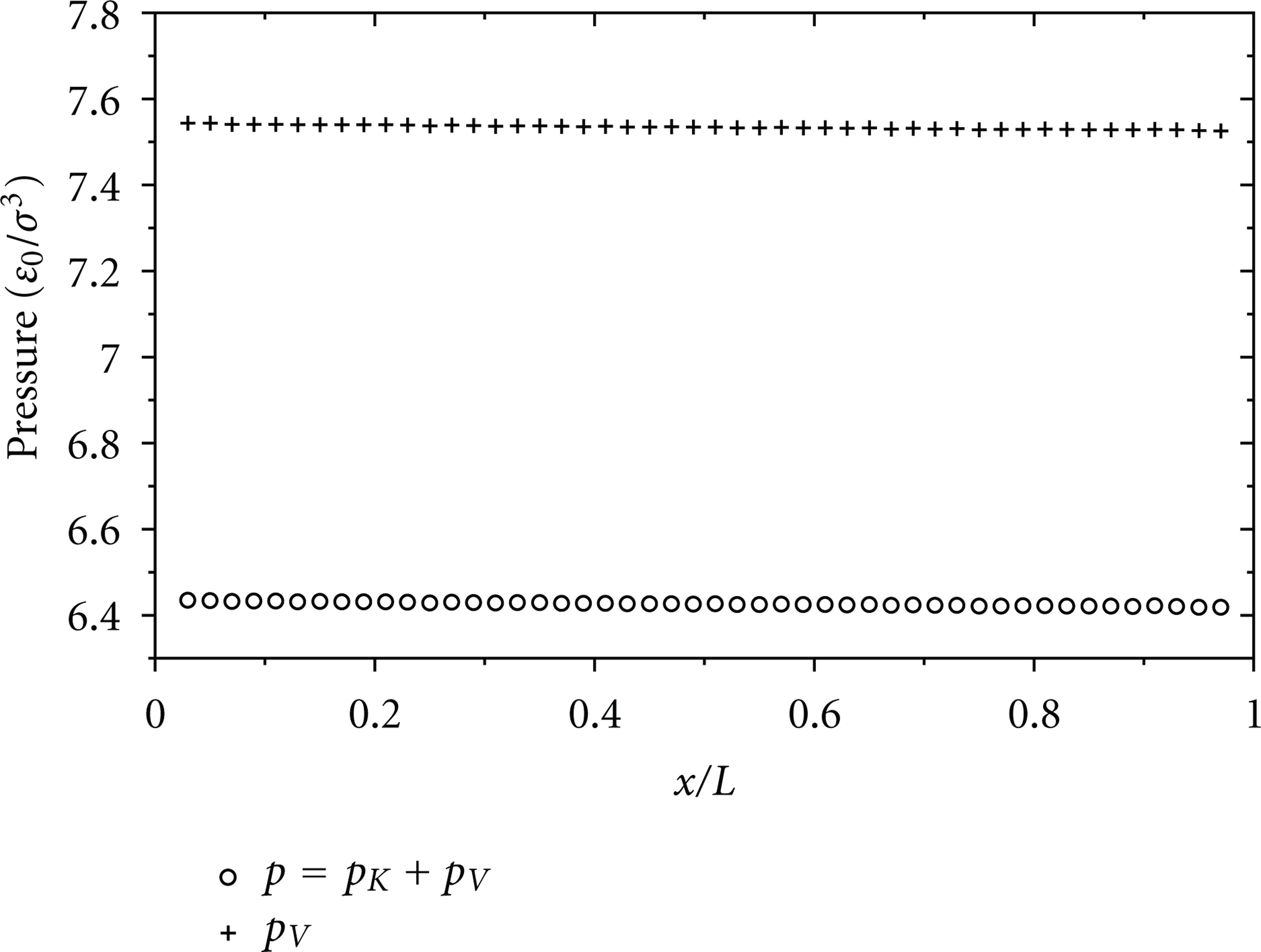
Axial variations of pressures
Next, we consider the velocity profiles across the channel section for these two cases. The velocity profiles (Figure 12) agree then with (3). The slip length for the case
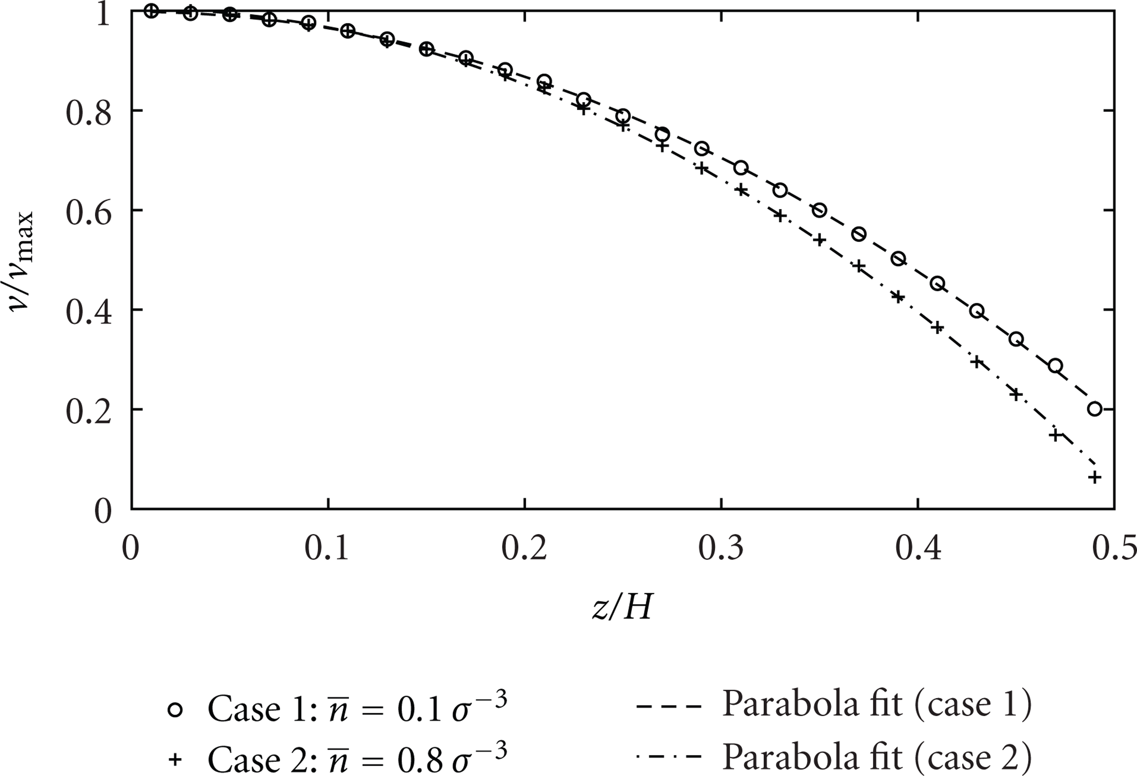
Dimensionless velocity profile in half of the channel cross-section for
It should thus be emphasized that the present method is relevant to generate various fluid flows even if we control only the difference between the inlet- and outlet-squared molecular velocities. The potential part p V , which depends on the interatomic interaction, can vary along the flow direction. As shown numerically, the variation of p V contributes considerably to the pressure gradient.
The third case aimed at modeling the flow within a rib-roughened channel. The parameters are the same as in the second case (

Streamlines in a rib-roughened channel. The color represents the fluid density field.

5. Conclusions
In this work, we have used a molecular dynamics method for simulating pressure-driven flows in channels. The main novelty lies in the modification of the periodic inlet and outlet velocity conditions: the difference in squared velocity between the ingoing and outgoing molecules of the simulation domain is maintained constant.
Plane Poiseuille flows were simulated, and the results were compared with approximate analytical solutions of the Navier-Stokes and energy equations reported in the literature. This new method has been proven to be realistic and could be applied to many problems with a nonconstant axial pressure gradient: flows around obstacles or in rough channels, for example. The method appears thus relevant for modeling compressibility effects as well as temperature variations along the flow direction, a domain unfulfilled by the usual molecular dynamics methods.