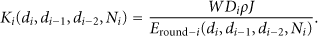
Sage Journals: Discover world-class research

Abstract

This paper addresses the cluster partitioning problem in wireless sensor networks deployed in a continuous area. We present the model of the network and describe its operational details firstly. Both single-hop and multihop transmissions with cooperative Multi-Input Single-Output (MISO) scheme are considered for the intercluster communications. Besides, uniform and linear data fusions are discussed. Then, the calculations of energy consumptions are derived. Different from other researches, the energy consumptions of intracluster communication in each cluster are included and modeled as functions of the cluster size. Finally, we simulate all possible cluster partitions by changing the numbers of clusters and cooperative transmitting nodes and find the maximal network lifetimes. As a result, the relationships between cluster partitions and network lifetimes are clarified in different situations.

1. Introduction

In recent researches, wireless sensor networks (WSNs) have witnessed a tremendous upsurge due to their great potential in many application domains, including industrial control, environment monitoring, and target tracking [1]. In some scenarios, a WSN needs to be deployed in continuous areas and the information collected is necessary to transmit to a base station (BS) periodically, such as traffic surveillance on highway and gas monitoring in mine tunnel [2].

In general, a WSN consists of large numbers of spatially distributed sensor nodes. These nodes are usually powered by small batteries with limited energy, for which replacement or recharging is quite difficult if not impossible. That is, finite energy can only support the transmission of a finite amount of information. Hence, minimizing energy consumptions and prolonging network lifetime are of great importance for the design of a WSN.

The clustering approach has been proved to be one of the most effective mechanisms to improve energy efficiency in WSNs [3]. In cluster-based WSNs, each cluster has a cluster head (CH) which can manage the nodes in the cluster. And the CH can execute data fusion (aggregation) to reduce the amount of data and save the overhead of intercluster transmission (from the cluster to the destination). For such cluster-based WSNs, many methods can be exploited to reduce energy consumptions of intercluster transmission [4]. Cooperative Multi-Input Multi-Output (MIMO) is one typical scheme of them.

The original MIMO scheme based on antenna arrays can achieve spatial diversity in fading channels, which requires less transmission power than noncooperative Single-Input Single-Output (SISO) scheme [5]. However, it is difficult to apply MIMO scheme directly in WSNs because of the limited sizes of nodes which can only support a single antenna. Fortunately, if multiple nodes in a cluster could cooperate on data transmission and reception, a cooperative MIMO scheme can be constructed to improve communication performance [6].

The authors of [6, 7] have proposed some cooperative MIMO schemes for single-hop transmission in a clustered WSN and analyzed their energy efficiency. It was shown that the number of cooperative nodes at both the transmission and reception sides should be selected with respect to the intercluster distance in order to minimize the total energy consumptions. Although a cooperative MIMO scheme can improve the system performance in terms of energy conservation, it cannot solve the energy imbalance of clusters caused by different transmission distances to the BS in single-hop WSNs. Using a cooperative transmitting (Multi-Input Single-Output, MISO) scheme, Bai et al. [8] have investigated the unequal cluster partitioning for single-hop transmission in a continuous area WSN so as to balance energy consumptions among the clusters and prolong the network lifetime.

According to the results of [8], clusters closer to the BS should have smaller sizes and the farther ones have larger sizes in single-hop WSNs because more energy consumptions for data transmitted to the BS are required with the increase of distances to the BS. However, in each cluster, energy consumptions of intracluster communication (between nodes and the CH) were ignored in the model of [8]. In reality, such energy consumptions will vary with the cluster size. Clusters with larger sizes need more energy consumptions for intracluster communication than those with smaller sizes. Furthermore, in [8], the amount of data after fusion in each cluster was assumed to be the same, which is not practical to describe some situations. It is possible that the information of nodes has not high correlations and each node has its different data. In such a case, the amount of data after fusion should increase with the cluster size.

Yuan et al. have extended the work in [6] and incorporated cooperative MIMO scheme with multihop networking [9]. Their results showed that cooperative MIMO scheme can be also effective in energy saving for multihop WSNs. In spite of that, similar to previous single-hop networks, the energy imbalance problem still exists in multihop WSNs. For example, in a network with equal divided clusters, the clusters closer to the BS may deplete their energy much faster than others because of higher traffic load. With consideration of the above problem, Mashreghi and Abolhassani [10] have developed an optimization model in a continuous area WSN and found the optimal parameters of the network, such as numbers of clusters and cooperative nodes, and cluster sizes.

It was shown in [10] that for multihop networks, the optimal cluster partition is the same as for single-hop in [8]: clusters farther from the BS should have larger sizes, but for different reason that clusters closer to the BS have to transmit more data and need shorter transmission distances. Nevertheless, the amount of data after fusion in each cluster has been considered also to be identical and independent of the cluster size in [10]. And the energy consumptions of intracluster communication never changed with the cluster size despite that it was considered.

This paper expands and develops the works in [8, 10]. In this paper, we discuss the cluster partitioning problem in single-hop and multihop WSNs deployed in a continuous area. Distinct from [8, 10], the energy consumptions of intracluster communication in each cluster are included and considered as functions of the cluster size in our model. Moreover, two kinds of data fusion are discussed, respectively. One is the conventional assumption, the uniform fusion, in which the amount of data after fusion is fixed as a constant. The other is the linear fusion, in which the amount of data after fusion increases linearly with the cluster size. To the best of our knowledge, this paper makes the first attempt at investigating the cluster partitioning with the linear fusion. By giving the length of the network, we change the numbers of clusters and cooperative transmitting nodes in each cluster and simulate all possible cluster partitions in order to investigate the variation of network lifetimes. As a result, we present the maximal network lifetimes and derive their relationships with cluster partitions in different situations. In our previous research [11], we have investigated the effect of cluster size on cluster lifetime in single-hop separated farmland WSNs. The analysis of [11] has been focused on a cluster, instead of the whole network and cluster partitioning. This is the difference between our previous work and this paper.

2. System Description

In this section, we present the network model and describe its operational details. To make our paper more readable, main symbols used are listed in Table 1.

Table 1

List of main symbols.

D	Length of network	k	Path loss factor
W	Width of network	C	Product of some communication constants
M	Number of clusters	$G_{T} G_{R}$	Tx and Rx antenna gains
$d_{i}$	Left boundary of ith cluster	λ	Carrier wavelength
$D_{i}$	Length of ith cluster	$M_{l}$	Link margin of RF amplifier
ρ	Node density	$N_{f}$	Receiver noise figure
L	Data amount per node	$N_{0}$	Thermal noise PSD
$Ω$	Coefficient about correlation	${\bar{P}}_{b}$	Average BER
γ	Data fusion ratio in linear fusion	$P_{CT}$	Power consumption of Tx circuits
$L_{F - i}$	Data amount after fusion in ith cluster	$P_{CR}$	Power consumption of Rx circuits
$N_{i}$	Number of cooperative transmitting nodes in ith cluster	$E_{A}$	Energy consumption per bit of data fusion
α	Constant about RF amplifier	$Δ$	Minimum step of cluster length
$R_{b}$	Transmission bit rate	J	Initial energy per node

2.1. Overview

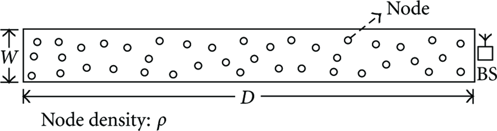
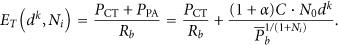
To investigate the aforementioned networks which can be used in traffic surveillance on highway and gas monitoring in mine tunnel, let us consider a simplified linear network where the BS is located at the right end and the sensor nodes are uniformly deployed in a continuous area with node density ρ, as illustrated in Figure 1. The length of the network D is much larger than the width W, and we can divide the whole network into M rectangle clusters. As shown in Figure 2, the position of the BS is $d_{0} = 0$ and $d_{i}$ is the distance between the left boundary of the ith cluster ( $i = 1,2, \dots, M$ ) and the BS. Thus, the area of the ith cluster is $W D_{i}$ , where $D_{i} = d_{i} - d_{i - 1}$ .

Figure 1

Network model.

Figure 2

Cluster partitioning of the network.

2.2. Operational Details

In the model of Figure 2, each cluster needs to report their data periodically to the BS by single-hop or multihop transmission. Without loss of generality, let us focus on the ith cluster to describe the operational details of the model. In each round, the following five steps will be executed successively in the ith cluster.

Step 1 (CH selection).

The system requires a CH to collect and fuse data of all nodes in the cluster and coordinate intercluster transmission. In view of the fact that the CH does more work than other nodes, it is necessary to select the node which has the most remaining energy to serve as the CH.

Step 2 (data gathering).

In this step, each node transmits its L bits of sensed data to the CH by a multiple access method, which is assumed to be perfect (no contention or retransmission).

Step 3 (data fusion).

After receiving the data from all nodes, the CH fuses (aggregates) these data based on their redundancy.

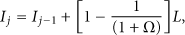
To calculate the amount of data after fusion in a cluster, an empirical equation obtained in [12] can give us some help. After a new source node, which is the jth node in a cluster, joins the existing set of nodes, the amount of fused data can approximately be calculated by

\begin{matrix} I_{j} = I_{j - 1} + [1 - \frac{1}{(1 + Ω)}] L, \end{matrix}

(1)

where

I_{j - 1}

is the amount of fused data generated by the existing set of nodes,

Ω = l_{j} / c

in which

l_{j}

is the minimum distance between the new source node and the existing set of nodes, and c is a constant and represents the degree of spatial correlation in the data. From this formula, we can find that the amount of data after fusion is always equal to L if the data has high correlation, that is,

Ω = 0

. Otherwise, the amount of data after fusion will increase with the number of nodes.

Hence, we discuss the uniform fusion and linear fusion, respectively, in the following sections. For simplicity, it is assumed that all nodes are distributed uniformly and the distances between adjacent nodes are identical. In the uniform fusion ( $Ω = 0$ ), the amount of data after fusion $L_{F - i}$ in the ith cluster is fixed as a constant and independent of the cluster size, which has been often used including [8, 10].

As for the linear fusion, we assume that the amount of data after fusion varies directly with the cluster size or the sum of corresponding nodes as

\begin{matrix} L_{F - i} = γ L ρ W D_{i} . \end{matrix}

(2)

In this equation, γ is the fusion ratio and set to 0.5 in the following sections, which corresponds to the case

Ω = 1

Step 4 (data broadcast).

In this step, the CH selects $N_{i} (N_{i} \geq 0)$ nodes which have more remaining energies to serve as cooperative transmitting nodes and then broadcasts the fused data to them if $N_{i} > 0$ . Besides, the CH needs to receive the data from the $(i + 1)$ th cluster and broadcast them to the cooperative transmitting nodes if the multihop transmission is used.

The case $N_{i} = 0$ means that noncooperative SISO scheme is used for the intercluster communication, and the CH alone transmits the data to the BS in single-hop transmission or the CH of the $(i - 1)$ th cluster in multihop transmission.

Step 5 (intercluster data transmission).

In this step, the CH and $N_{i}$ cooperative transmitting nodes use a Space-Time Block Code (STBC) [13] to encode the data and transmit them simultaneously to the BS or the next CH.

3. Energy Consumptions

In this section, we introduce the calculation of energy consumptions in our model.

3.1. Energy Consumptions of a Node

Here, we use a simple model in which the total energy consumptions of a node can be categorized into two main parts, the energy consumption of the transmission mode and that of the reception mode. This model is widely validated and used by researchers in [6–10].

3.1.1. For Data Transmission

When a node transmits data, its transmission circuits will work. As shown in Figure 3, this part of circuits includes the D/A converter (DAC), the mixer, the active filters, the frequency synthesizer (LO), and the power amplifier (PA) [14]. For the simplicity of estimation, the digital signal processing blocks (coding, pulse-shaping, digital modulation, and so on) are omitted. Except the power amplifier, the power consumptions of all the other blocks are regarded as constants and we use $P_{CT}$ to represent the summation of these power consumptions.

Figure 3

Transmission circuits of a node.

According to [14], the power consumption of the power amplifier $P_{PA}$ can be approximated as

\begin{matrix} P_{PA} = (1 + α) P_{out}, \end{matrix}

(3)

where

α = ξ / η - 1

with η the drain efficiency of the RF power amplifier and ξ the peak-to-average ratio. The transmission power

P_{out}

can be calculated from the link budget relationship [15] as

\begin{matrix} P_{out} = \frac{C \cdot E_{b} R_{b} d^{k}}{1 + N_{i}}, \end{matrix}

(4)

where

E_{b}

is the required energy per bit at the receiver for the given bit error ratio (BER) requirement,

R_{b}

is the transmission bit rate, d is the transmission distance, and k is the path loss factor. In addition, for the intracluster communication, cooperative transmission is not used and

N_{i} = 0

In (4), C is the product of various communication constants which is defined as

\begin{matrix} C = \frac{{(4 π)}^{2}}{G_{T} G_{R} λ^{2}} M_{l} N_{f} . \end{matrix}

(5)

The detailed meanings of these constants are given in Table 1.

Although all nodes are fixed, the environment is mutable, for example, the movement of vehicles or human can affect the channel. In such a case, the channel can be regarded as fading channel. Hence, let us assume that the network operates under a flat slow Rayleigh-fading channel, that is, the channel gain is a scalar. In other words, on top of the k-law path loss, the signals are further attenuated by a scalar fading matrix H, in which the elements are independent zero mean circularly symmetric complex Gaussian (ZMCSCG) random variables with unit variance [5]. Furthermore, BPSK is assumed as the modulation scheme during data transmission, and, from [15], the BER of BPSK modulation is

\begin{matrix} P_{b} = Q (\sqrt{2 γ_{b}}), \end{matrix}

(6)

where

γ_{b}

is the instantaneous received signal to noise ratio (SNR). Since cooperative transmitting nodes use STBC to transmit the data, the receiver can obtain similar performance to maximal-ratio combining (MRC) scheme and

γ_{b}

can be given by

\begin{matrix} γ_{b} = \frac{{‖ H ‖}_{F}^{2}}{1 + N_{i}} \frac{E_{b}}{N_{0}}, \end{matrix}

(7)

where

∥ H ∥_{F}^{2}

is the squared Frobenius norm of H and

N_{0}

is the single-sided thermal noise power spectral density (PSD). Hence, the average BER

{\bar{P}}_{b}

can be estimated as follows:

\begin{matrix} {\bar{P}}_{b} = E_{H} {Q (\sqrt{2 γ_{b}})}, \end{matrix}

(8)

where

E_{H} {x}

represents the average value of x over H. Applying the Chernoff bound [15], an upper bound of

E_{b}

is given by

\begin{matrix} E_{b} \leq \frac{N_{0} (1 + N_{i})}{{\bar{P}}_{b}^{1 / (1 + N_{i})}} . \end{matrix}

(9)

By approximating this bound as an equality, we obtain an expression for

E_{b}

using

{\bar{P}}_{b}

, and

P_{PA}

can be expressed by

\begin{matrix} P_{PA} = \frac{(1 + α) C \cdot N_{0} R_{b} d^{k}}{{\bar{P}}_{b}^{1 / (1 + N_{i})}} . \end{matrix}

(10)

Therefore, when a node transmits data, the energy consumption per bit can be calculated by

\begin{matrix} E_{T} (d^{k}, N_{i}) = \frac{P_{CT} + P_{PA}}{R_{b}} = \frac{P_{CT}}{R_{b}} + \frac{(1 + α) C \cdot N_{0} d^{k}}{{\bar{P}}_{b}^{1 / (1 + N_{i})}} . \end{matrix}

(11)

3.1.2. For Data Reception

Figure 4 shows the reception circuits of a node, which consist of the filters, the low-noise amplifier (LNA), the mixer, the LO, the intermediate frequency amplifier (IFA), and the A/D converter (ADC) [14]. In our model, the power consumptions of all these blocks are also regarded as constants and we use $P_{CR}$ to represent the summation of them.

Figure 4

Reception circuits of a node.

Hence, when a node receives data, the energy consumption per bit is given by

\begin{matrix} E_{R} = \frac{P_{CR}}{R_{b}} . \end{matrix}

(12)

3.2. Energy Consumptions of a Cluster

Using $E_{T} (d^{k}, N_{i})$ and $E_{R}$ defined above, let us calculate the energy consumptions of the ith cluster per round. We assume that each node can adjust the transmission power based on its distance to the destination in order to save energy consumptions.

Step 1 (CH selection).

This step is assumed to be completed by the BS, in which the energy is unrestrained. And it is noted that when all nodes receive the message from the BS that which one will serve as the CH, some energy consumptions are required. However, these energy consumptions are independent of the cluster partitioning since they are mandatory and identical for all nodes. Hence, we ignore them in the following discussion.

Step 2 (data gathering).

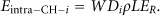
In this step, all nodes send their data and the CH receives them. Since any node can act as the CH, the position of the CH is not fixed. To calculate the total energy consumptions of all nodes, average path loss of intracluster communication is used in our model. In detail, the average path loss is denoted as

\begin{matrix} {\bar{d^{k}}}_{intra - i} = \frac{1}{W D_{i}} \iint_{W D_{i}}^{} {(u^{2} + v^{2})}^{k / 2} d u d v . \end{matrix}

(13)

The upper and lower limits of integration depend on the position of the CH. Hence, the total energy consumptions of all nodes in this step can be expressed as

\begin{matrix} E_{intra - i} (d_{i}, d_{i - 1}) = W D_{i} ρ L E_{T} ({\bar{d^{k}}}_{intra - i}, 0) . \end{matrix}

(14)

Moreover, the receiving energy consumption of the CH in this step can be calculated from

\begin{matrix} E_{intra - CH - i} = W D_{i} ρ L E_{R} . \end{matrix}

(15)

Step 3 (data fusion).

After receiving the data from all nodes, the CH fuses these data. The energy consumption of data fusion at the CH can be represented as

\begin{matrix} E_{fusion - CH - i} = W D_{i} ρ L E_{A}, \end{matrix}

(16)

where

E_{A}

is the energy consumption per bit of data fusion and depends on the algorithm complexity. For simplicity, we use the experiment result in [16] and assume

E_{A} = 5

nJ/bit.

Step 4 (data broadcast).

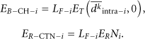
In this step, if the single-hop transmission is used, the CH broadcasts the fused data and the cooperative transmitting nodes receive them. The energy consumptions of the CH and all cooperative transmitting nodes can be represented, respectively, as

\begin{gathered} \begin{matrix} E_{B - CH - i} = L_{F - i} E_{T} ({\bar{d^{k}}}_{intra - i}, 0), \end{matrix} \\ E_{R - CTN - i} = L_{F - i} E_{R} N_{i} . \end{gathered}

(17)

If the multihop transmission is used, besides broadcasting the data of its cluster, the CH must receive the data from the 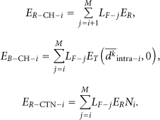$(i + 1)$ th cluster and broadcast them to the cooperative transmitting nodes. In this case, the energy consumptions of the CH and all cooperative transmitting nodes can be written by

\begin{gathered} \begin{matrix} E_{R - CH - i} = \sum_{j = i + 1}^{M} L_{F - j} E_{R}, \end{matrix} \\ E_{B - CH - i} = \sum_{j = i}^{M} L_{F - j} E_{T} ({\bar{d^{k}}}_{intra - i}, 0), \\ E_{R - CTN - i} = \sum_{j = i}^{M} L_{F - j} E_{R} N_{i} . \end{gathered}

(18)

Step 5 (intercluster data transmission).

In this step, the CH and cooperative transmitting nodes transmit the data to the BS or the next CH cooperatively. Accordingly, we obtain the total energy consumptions in this step as follows. (i)

In single-hop transmission,

\begin{matrix} E_{inter - i} (d_{i}, d_{i - 1}, N_{i}) = (1 + N_{i}) L_{F - i} E_{T} ({\bar{d^{k}}}_{inter - s - i}, N_{i}), \end{matrix}

(19)

where the average path loss of intercluster communication in single-hop transmission is calculated by

\begin{matrix} {\bar{d^{k}}}_{inter - s - i} = \frac{1}{W D_{i}} \int_{- W / 2}^{W / 2} \int_{d_{i - 1}}^{d_{i}} {(u^{2} + v^{2})}^{k / 2} d u d v . \end{matrix}

(20)

(ii)

In multihop transmission,

\begin{matrix} E_{inter - i} (d_{i}, d_{i - 1}, d_{i - 2}, N_{i}) \\ \begin{matrix} = (1 + N_{i}) \sum_{j = i}^{M} L_{F - j} E_{T} ({\bar{d^{k}}}_{inter - m - i}, N_{i}), \end{matrix} \end{matrix}

(21)

where the average path loss of intercluster communication in multihop transmission can be expressed as

\begin{matrix} {\bar{d^{k}}}_{inter - m - i} \\ = {\begin{cases} \frac{1}{W D_{1}} \int_{- W / 2}^{W / 2} \int_{0}^{d_{1}} {(u^{2} + v^{2})}^{k / 2} d u d v, \\ for i = 1, \\ \frac{1}{W D_{i}} \int_{- W / 2}^{W / 2} \int_{d_{i - 1} - (d_{i - 1} + d_{i - 2}) / 2}^{d_{i} - (d_{i - 1} + d_{i - 2}) / 2} {(u^{2} + v^{2})}^{k / 2} d u d v, \\ for 2 \leq i \leq M . \end{cases} \end{matrix}

(22)

Here, we assume that the CH of the

(i - 1)

th cluster (

2 \leq i \leq M

) is located in the center of the cluster to simplify our calculations.

To sum up the above energy consumptions of all five steps, we achieve the total energy consumptions of the ith cluster per round, which is represented by $E_{round - i} (d_{i}, d_{i - 1}, d_{i - 2}, N_{i})$ .

4. Lifetime Definitions

In this section, we give the definitions of lifetimes and present the problem of cluster partitioning.

4.1. Cluster Lifetime

In our model, it is assumed that the CH and cooperative transmitting nodes are selected from all nodes based on their remaining energies. Therefore, on the whole, we consider that the energy consumptions among all nodes in a cluster are to be balanced and all nodes have equal lifetimes approximately. If we assume that each node has J joules in its battery, the lifetime of the ith cluster can be defined as the possible total transmission rounds, which can be calculated by

\begin{matrix} \begin{matrix} K_{i} (d_{i}, d_{i - 1}, d_{i - 2}, N_{i}) = \frac{W D_{i} ρ J}{E_{round - i} (d_{i}, d_{i - 1}, d_{i - 2}, N_{i})} . \end{matrix} \end{matrix}

(23)

4.2. Network Lifetime

In clustered WSNs, the data of all nodes in a cluster is fused by the CH for reducing the redundancy and then transmitted to the BS. From the BS's point of view, every cluster can be regarded as the unit which transmits data. If any cluster dies, the network will lose the coverage of corresponding area. Hence, the network lifetime is defined as the minimum lifetime of clusters in our model:

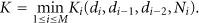
\begin{matrix} \begin{matrix} K = \min_{1 \leq i \leq M} K_{i} (d_{i}, d_{i - 1}, d_{i - 2}, N_{i}) . \end{matrix} \end{matrix}

(24)

According to (24), we find that different cluster partitions and numbers of cooperative transmitting nodes may result in different network lifetimes. For the sake of maximizing network lifetime, it is necessary to investigate the appropriate cluster partitions and cooperative MISO schemes, which will be clarified below. It is noted that the cluster partitioning is a multivariable and discrete function, which means that the analytic results are hard to derive. So it is expected that some qualitative conclusions can be derived from our simulation results.

5. Numerical Results

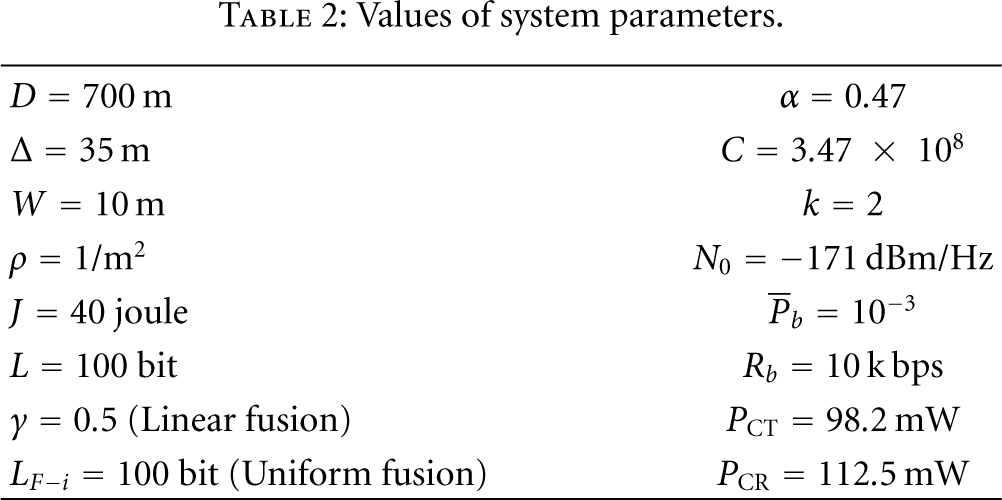
In this section, let us operate the simulations and analyze their results. The system parameters used in our simulations are shown in Table 2. Although the following simulations are executed under a given length of network $D = 700$ meters, our conclusions can be validated by other values of parameters. Furthermore, minimum step size or resolution of the cluster length $D_{i}$ is set to be $Δ$ , which is a divisor of D. Accordingly, the maximal number of clusters is $D / Δ$ (=20). Such assumption will lead to approximate results, but it does not affect our final conclusions. As for (13), to make our results reasonable, we calculate the integration over 5000 randomly generated positions of the CH for every size of the cluster and use the average values of them. In the following simulations, for every number of clusters, we first consider all possible cluster partitions then find the maximal network lifetimes based on (24).

Table 2

Values of system parameters.

$D = 700$ m	$α = 0.47$
$Δ = 35$ m	$C = 3.47 \times 1 0^{8}$
$W = 10$ m	$k = 2$
$ρ = 1$ / $m^{2}$	$N_{0} = - 171$ dBm/Hz
$J = 40$ joule	${\bar{P}}_{b} = 1 0^{- 3}$
$L = 100$ bit	$R_{b} = 10$ k bps
$γ = 0.5$ (Linear fusion)	$P_{CT} = 98.2$ mW
$L_{F - i} = 100$ bit (Uniform fusion)	$P_{CR} = 112.5$ mW

5.1. Single-Hop Transmission

5.1.1. The Uniform Fusion

We change the number of clusters from 1 to 20 and calculate all possible cluster partitions then derive Figure 5, which shows the maximal network lifetimes in single-hop transmission with the uniform fusion. From this figure, it can be found that the maximal network lifetimes increase with the number of clusters. The reason lies in the fact that, with the uniform fusion, the amount of data after fusion in each cluster is small (100 bits) so that the energy consumptions of intercluster communication is relatively minor compared with those of intracluster communication. Consequently, larger numbers of clusters make these clusters with smaller sizes, which decrease their energy consumptions of intracluster communications and obtain longer lifetimes.

Figure 5

Maximal network lifetimes with different numbers of clusters in single-hop transmission (the uniform fusion).

Table 3 shows the optimal numbers of cooperative transmitting nodes and optimal cluster sizes with $M = 6$ . It is observed that the clusters farther from the BS need larger numbers of cooperative transmitting nodes $N_{i}$ , which is in accord with the results of previous works [6, 7]. But more important is that such farther clusters do not have larger sizes, which is entirely different from the former results in [8]. Instead, they should have smaller size, as shown in Table 3. In fact, the increase of the cluster size reduces the possibility of nodes joining the intercluster communication, but it also makes the cluster consume more energies in its intracluster communication. As was mentioned above, since the data transmitted of the intercluster communication is small in the uniform fusion, the intracluster communication plays a major role. Thus, the clusters farther from the BS should be arranged with smaller sizes.

Table 3

Optimal cluster partition when the number of clusters $M = 6$ in single-hop transmission (the uniform fusion).

Cluster i	1	2	3	4	5	6
$N_{i}$	0	1	1	2	2	2
$D_{i}$ (m)	140	140	105	105	105	105

5.1.2. The Linear Fusion

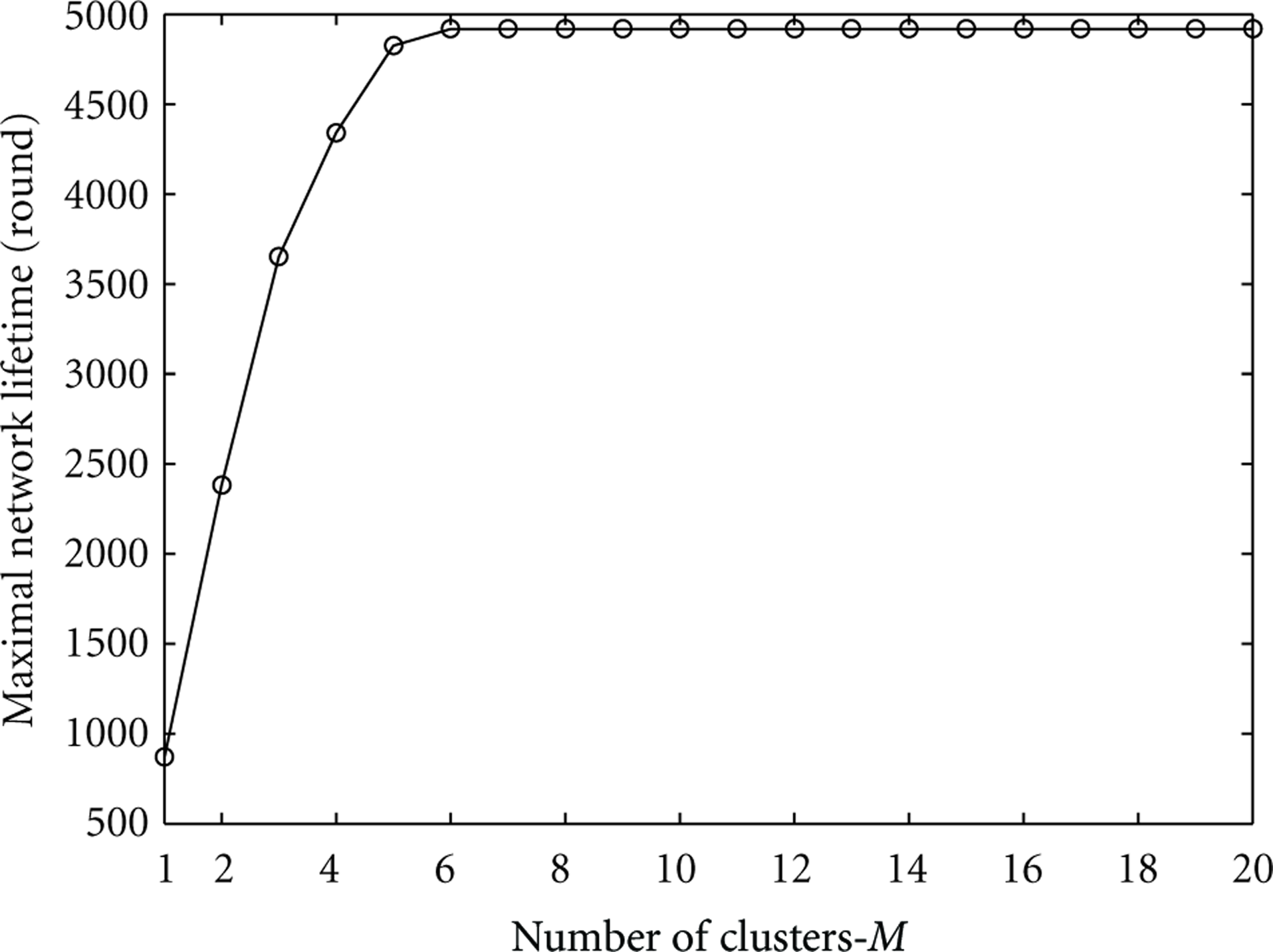
When the linear fusion is applied, by changing the number of clusters M from 1 to 20, we depict the maximal network lifetimes of single-hop transmission in Figure 6. From this figure, we can see that the maximal network lifetime increases with the number of clusters and saturates at $M = 6$ in the linear fusion. When M is small, it is difficult to balance the lifetimes of clusters and the clusters need more energy consumptions of intracluster communication because of their assigned larger sizes. But this situation will be eased by the increase of M. Therefore, the maximal network lifetimes raise when M changes from 1 to 6, as shown in Figure 6.

Figure 6

Maximal network lifetimes with different numbers of clusters in single-hop transmission (the linear fusion).

Now let us put an emphasis on the case $M = 6$ . Table 4 presents the optimal cluster partition and corresponding cluster lifetimes when the number of clusters $M = 6$ . Similar to the result of uniform fusion, the clusters farther from the BS have larger numbers of cooperative transmitting nodes. Furthermore, they are arranged with smaller sizes. In the linear fusion, if the cluster size increases, besides the energy consumptions of intracluster communication, the amount of data after fusion will also increase. So it is impossible for the farther clusters to reduce the energy consumptions of intercluster communications and realize longer lifetimes by increasing their sizes. On the contrary, they will benefit from smaller sizes which can save the energy consumptions of intracluster communications.

Table 4

Optimal cluster partition when the number of clusters $M = 6$ in single-hop transmission (the linear fusion).

Cluster i	1	2	3	4	5	6
$N_{i}$	0	1	2	2	2	2
$D_{i}$ (m)	175	175	140	105	70	35
$K_{i}$ (round)	6321	5299	5079	5068	4990	4917

From Table 4, we can also judge that the Mth cluster determines the maximal network lifetime when the number of clusters $M = 6$ . In fact, since the left boundary of the Mth cluster is fixed at D, reducing its size means decreasing the energy consumptions of intracluster communication, while increasing its average distance from the BS. That brings up a trade off which causes that the lifetime of this cluster has an extremum. Figure 7 shows our simulation result for the lifetime of the Mth cluster specially. In this figure, a smaller simulation resolution $Δ = 5$ meters is used to find the extremum lifetime of the Mth cluster. We find that there definitely exists a maximal lifetime of the Mth cluster at $D_{M} = 25$ meters.

Figure 7

Maximal lifetimes of the Mth cluster in single-hop transmission (the linear fusion).

In Figure 6, the maximal network lifetime remains unchanged when $M \geq 6$ . This is because of the limitation in the minimum cluster size. When $M \geq 6$ , the Mth cluster always has a length $Δ = 35$ meters in the optimal cluster partitions. The fact indicates again that the farthest cluster determines the maximal network lifetime. And the maximal lifetime of this cluster is also the possible maximal network lifetime in single-hop transmission when the linear fusion is used.

5.2. Multihop Transmission

5.2.1. The Uniform Fusion

Figure 8 shows the maximal network lifetimes with different numbers of clusters in multihop transmission if the uniform fusion is used. Similar to the results of single-hop transmission shown in Figure 5, when the uniform fusion is employed, the energy consumptions of intracluster communication are more dominant than those of intercluster because of larger amount of data transmitted. Hence, with the increase of M, the clusters are arranged with smaller sizes, which means that less energy consumptions of intracluster communication are required. And the maximal network lifetimes increase accordingly, as shown in Figure 8.

Figure 8

Maximal network lifetimes with different numbers of clusters in multihop transmission (the uniform fusion).

5.2.2. The Linear Fusion

Next let us focus on the linear fusion again. We show the maximal network lifetimes in Figure 9. Similar to Figure 6, as M raises from 1, the maximal network lifetimes increase with the same reason.

Figure 9

Maximal network lifetimes with different numbers of clusters in multihop transmission (the linear fusion).

When the number of clusters $M = 4$ , we get the maximum of network lifetime. The corresponding six sets of optimal cluster partitions are presented in Figure 10. It is interesting that among these optimal partitions, the sizes of the first and second clusters are fixed while those of other clusters can change. This implies that the maximal network lifetime in multihop transmission is determined by the first and second clusters. Moreover, when M increases from 4 to 12, the sizes of the first and second clusters remain unchanged (140 and 210 meters) in all optimal partitions so that the network always has its maximal lifetime, as shown in Figure 9. This demonstrates that there exists a special combination of the clusters closer to the BS which can maximize the network lifetime. In fact, after considering the energy consumptions of intracluster communication as the functions of the cluster sizes, a trade-off occurs among the clusters closer to the BS. For example, smaller size of the first cluster makes its energy consumptions of intracluster and intercluster communications smaller. On the other hand, larger size of the first cluster with larger number of nodes provides smaller chance for each node to be involved in the intercluster communication. Hence, a preferred combination is necessary for the clusters closer to the BS.

Figure 10

Six optimal cluster partitions when the number of clusters $M = 4$ in multihop transmission (the linear fusion).

When M continues to increase from 12, the sizes of the first and second clusters have to deviate from the preferred combination in order to satisfy the given M. Hence, the maximal network lifetimes also decrease gradually. Furthermore, we change the length of network and obtain similar simulation results.

6. Conclusions

In this paper, we have investigated the cluster partitioning with cooperative MISO scheme in a continuous area WSN. Unlike existing works in this field, this paper has included the energy consumptions of intracluster communication as the functions of the cluster sizes. Both single-hop and multihop transmissions have been considered for the intercluster communications. Moreover, the uniform and linear data fusions also have been discussed in the model.

By numerical simulations, we have presented the network lifetimes in various situations. If the uniform fusion is considered, the network lifetime increases with the number of clusters in either single-hop or multihop transmission. And the clusters farther from the base station should be assigned with smaller sizes in single-hop transmission. As for the case of linear fusion, our conclusions depend on the transmission schemes: in single-hop transmission, the optimal cluster partition indicates that the cluster size decreases with the increase of its distance to the base station, and the farthest cluster determines the maximal network lifetime; in multihop transmission, the clusters closer to the base station have a preferred combination which maximizes the network lifetime. Although this paper has focused on the one-dimension model, a two-dimension network can be divided into one-dimension networks. Hence, the conclusions derived here can be extended into the two-dimension situations.

References

Akyildiz

I. F.

Sankarasubramaniam

Cayirci

A survey on sensor networks

IEEE Communications Magazine 2002 40 8 102 114

2-s2.0-0036688074

10.1109/MCOM.2002.1024422

Tilak

B. Abu-Ghazaleh

Heinzelman

A taxonomy of wireless micro-sensor network models

ACM SIGMOBILE Mobile Computing and Communications Review 2002 6 2 28 36

Bandyopadhyay

Coyle

E. J.

An energy efficient hierarchical clustering algorithm for wireless sensor networks

Proceedings of the 22nd Annual Joint Conference of the IEEE Computer and Communications (INFOCOM ′03)

March 2003

San Francisco, Calif, USA

1713 1723

Raghunathan

Ganeriwal

Srivastava

Emerging techniques for long lived wireless sensor networks

IEEE Communications Magazine 2006 44 4 108 114

2-s2.0-33646949477

10.1109/MCOM.2006.1632657

Paulraj

Nabar

Gore

Introduction to Space-Time Wireless Communications 2003

Cambridge, UK

Cambridge University Press

Cui

Goldsmith

A. J.

Bahai

Energy-efficiency of MIMO and cooperative MIMO techniques in sensor networks

IEEE Journal on Selected Areas in Communications 2004 22 6 1089 1098

2-s2.0-4344710765

10.1109/JSAC.2004.830916

Nguyen

T. D.

Berder

Sentieys

Cooperative MIMO schemes optimal selection for wireless sensor networks

Proceedings of the IEEE 65th Vehicular Technology Conference (VTC ′07)

April 2007

Dublin, Ireland

85 89

Bai

Zhao

Liao

Energy balance in cooperative wireless sensor network

Proceedings of the 14th European Wireless Conference (EW ′08)

June 2008

Prague, Czech

1 5

2-s2.0-57849086868

10.1109/EW.2008.4623879

Yuan

Chen

Virtual MIMO-based cross-layer design for wireless sensor networks

IEEE Transactions on Vehicular Technology 2006 55 3 856 864

2-s2.0-33744547103

10.1109/TVT.2006.873837

10.

Mashreghi

Abolhassani

Prolongation of lifetime for wireless sensor networks by a cooperative MIMO system

Proceedings of the IEEE 3rd International Conference on Intelligent Sensors, Sensor Networks andInformation Processing (ISSNIP 07)

December 2007

Melbourne, Australia

73 78

11.

Huang

Kobayashi

Katayama

Yamazato

A study on cluster lifetime of single-hop wireless sensor networks with cooperative MISO scheme

IEICE Transactions on Communications 2011 94 10 2881 2885

12.

Pattem

Krishnamachari

Govindan

The impact of spatial correlation on routing with compression in wireless sensor networks

Proceedings of the 3rd International Symposium on Information Processing in Sensor Networks

April 2004

Los Angeles, Calif, USA

28 35

13.

Tarokh

Jafarkhani

Calderbank

A. R.

Space-time block codes from orthogonal designs

IEEE Transactions on Information Theory 1999 45 5 1456 1467

2-s2.0-0032656952

10.1109/18.771146

14.

Cui

Goldsmith

A. J.

Bahai

Energy-constrained modulation optimization

IEEE Transactions on Wireless Communications 2005 4 5 2349 2360

2-s2.0-26844485330

10.1109/TWC.2005.853882

15.

G. Proakis

Digital Communications 2000 4th

New York, NY, USA

McGraw-Hill

16.

Wang

Heinzelman

Chandrakasan

Energy-scalable protocols for battery-operated microsensor networks

Proceedings of the IEEE Workshop on Signal Processing Systems

1999

Taipei, Taiwan

483 492

A Study on Cluster Partitioning with Cooperative MISO Scheme in Wireless Sensor Networks

Abstract

1. Introduction

2. System Description

2.1. Overview

2.2. Operational Details

Step 1 (CH selection).

Step 2 (data gathering).

Step 3 (data fusion).

Step 4 (data broadcast).

Step 5 (intercluster data transmission).

3. Energy Consumptions

3.1. Energy Consumptions of a Node

3.1.1. For Data Transmission

3.1.2. For Data Reception

3.2. Energy Consumptions of a Cluster

Step 1 (CH selection).

Step 2 (data gathering).

Step 3 (data fusion).

Step 4 (data broadcast).

Step 5 (intercluster data transmission).

4. Lifetime Definitions

4.1. Cluster Lifetime

4.2. Network Lifetime

5. Numerical Results

5.1. Single-Hop Transmission

5.1.1. The Uniform Fusion

5.1.2. The Linear Fusion

5.2. Multihop Transmission

5.2.1. The Uniform Fusion

5.2.2. The Linear Fusion

6. Conclusions

References