Experimental Validation of Volume of Fluid Method for a Sluice Gate Flow

Abstract

Laboratory experiments are conducted for 2D turbulent free surface flow which interacts with a vertical sluice gate. The velocity field, on the centerline of the channel flow upstream of the gate is measured using the particle image velocimetry technique. The numerical simulation of the same flow is carried out by solving the governing equations, Reynolds-averaged continuity and Navier-Stokes equations, using finite element method. In the numerical solution of the governing equations, the standard $k-\epsilon$ turbulence closure model is used to define the turbulent viscosity. The measured horizontal velocity distribution at the inflow boundary of the solution domain is taken as the boundary condition. The volume of fluid (VOF) method is used to determine the flow profile in the channel. Taking into account of the flow characteristics, the computational domain is divided into five subdomains, each having different mesh densities. Three different meshes with five subdomains are employed for the numerical model. A grid convergence analysis indicates that the discretization error in the predicted velocities on the fine mesh remains within 2%. The computational results are compared with the experimental data, and, the most suitable mesh in predicting the velocity field and the flow profile among the three meshes is selected.

1. Introduction

The laboratory experiments on physical models of flow phenomena which have interactions with various types of hydraulic structures may be expensive and time consuming, and also the results are bound to be somewhat scale-affected. On the other hand, the computational fluid dynamics (CFDs) simulation of flow fields may be capable of providing precise solutions for the efficient designing of hydraulic structures.

According to the results of CFD studies in recent years, the volume of fluid (VOF) method, which provides a simple way of treating the topological changes of the air-water interface in free-surface flows, appears to be a powerful computational tool for the analysis of steady and unsteady free-surface flows interacting with spillways, weirs, and wall type hydraulic structures [1, 2]. The numerical results for turbulent flows so far obtained from the experimental validations on physical models [3–10] and on prototypes [11] show that the VOF-based CFD modeling is capable of investigating the performance of hydraulic structures. However, from the results of VOF-based numerical simulations so far, it seems that further experimental validations are useful before this method is confidently applied to the future studies of different free-surface flows.

In predicting the various characteristics of flow under the gates that are widely used hydraulic structures for controlling and metering the open channel flow, many experimental and theoretical studies have recently been undertaken [12–15]. The present work is concerned with the experimental validation of the VOF-based finite element analysis of the rectangular open channel flow interacting with a vertical sluice gate. Using particle image velocimetry (PIV) technique, laboratory experiments were conducted to determine the velocity field of 2D flow upstream of the gate. The computational results for the velocity field and the free-surface profile obtained from the VOF-based CFD modeling, were compared with the experimental data.

2. Experiments

The experiments were conducted in a glass-walled (including the bed), hydraulically smooth, horizontal laboratory channel which was 2.4 m long with cross-sectional dimensions of $0.2\times 0.2$ m. A smooth, sharp-edged vertical sluice gate model with 2 mm thickness was mounted in the channel. The experimental conditions of the flow are shown in Figure 1 and given in Table 1, where Q is the discharge, h₀ is upstream subcritical flow depth, a is gate opening from the channel bed, h _c is flow depth at the contraction section of the rapidly varied flow under the gate, L _c is the contraction length, C _c is the contraction coefficient, C _d is the discharge coefficient, Fr₀ is Froude number, and Re₀ is Reynolds number. The discharge was measured using a volumetric tank. In Table 1, $V_0=Q/(b{h}_0)$ is average velocity, b is channel width, R₀ is hydraulic radius of upstream flow, g is gravitational acceleration, and $\nu$ is kinematic viscosity of water.

Table 1:

Experimental conditions.

Q(L/s)	$h_{\mathrm{0}}$ (mm)	a(mm)	h c (mm)	L c (mm)	$C_c=h_c/a$	$C_d=Q/[ba{(\mathrm{2}g{h}_{\mathrm{0}})}^{\mathrm{1}/\mathrm{2}}]$	${\text{Fr}}_{\mathrm{0}}=V_{\mathrm{0}}/{(g{h}_{\mathrm{0}})}^{\mathrm{1}/\mathrm{2}}$	${\mathrm{Re}}_{\mathrm{0}}=\mathrm{4}{V}_{\mathrm{0}}{R}_{\mathrm{0}}/\nu$
1.7	64	12	8.3	14	0.69	0.63	0.17	19 930

Figure 1:

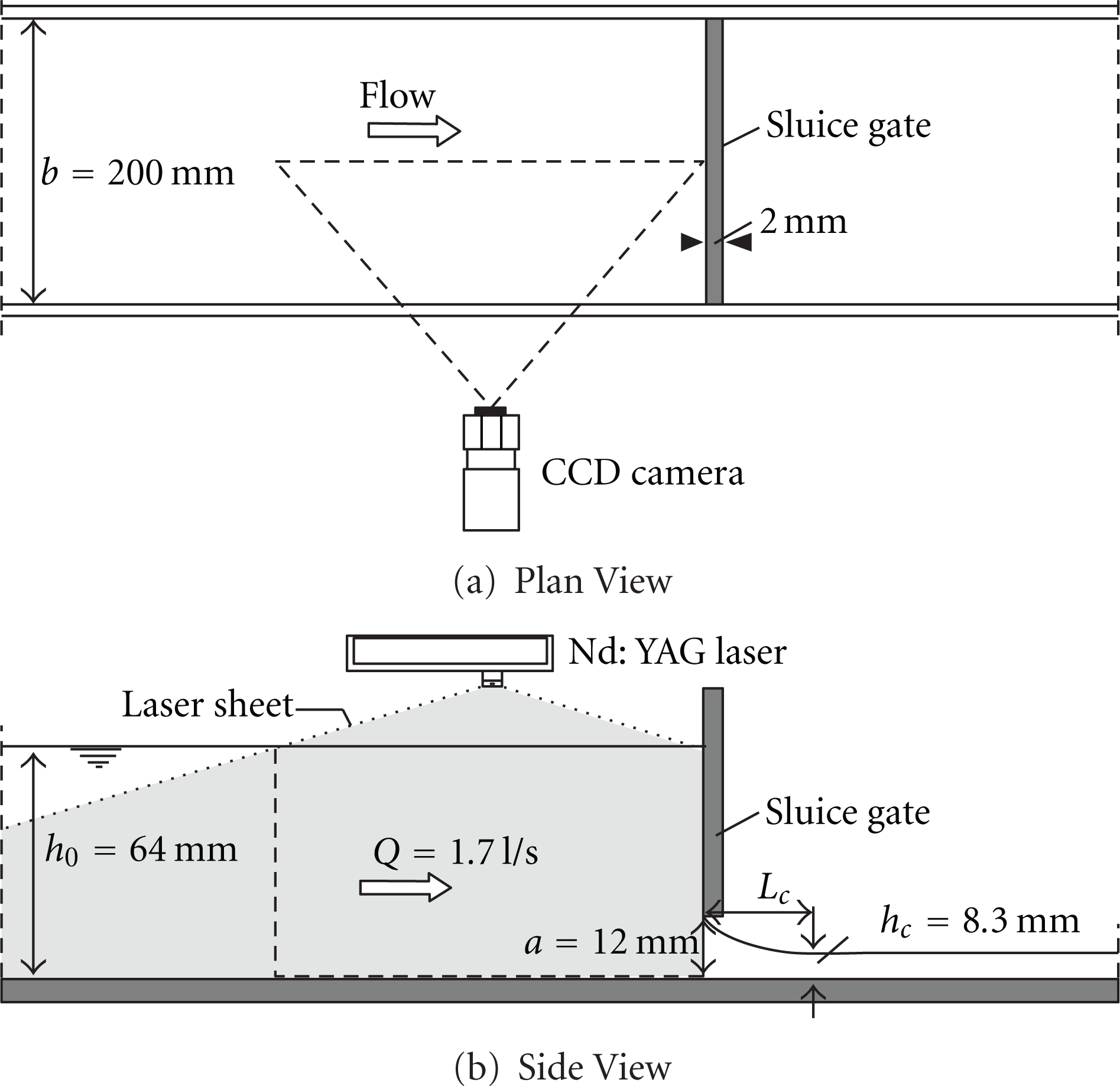
Experimental arrangement for velocity measurement using PIV system.

For measuring the flow velocities, various experimental techniques such as the laser doppler anemometry [16], particle image velocimetry [17], and acoustic doppler velocimetry [18] have been employed in recent years. In the present study, the flow velocities were measured using the particle image velocimetry (PIV) technique. The experimental arrangement for the measurement of velocity field upstream of the vertical gate is shown in Figure 1. The instantaneous velocities of the flow field at the mid-span of the channel were measured using the Dantec PIV flow measuring system. The flow was illuminated via a 2 mm thick laser sheet from a pair of double-pulsed Nd:YAG laser unit. Within the 2D measuring area of the flow, the velocity vectors were determined by recording the displacements of the seeding particles between the two locations during a specified time intervals of the two pulses which were 2.5 ms. The movement of the particles were recorded by a CCD camera with a resolution of 1024×1024 pixels. From the recorded particle image velocity data, the displacement vectors were obtained. The size of the velocity measuring field viewed by the laser sheet was $222.5\times 224.3$ mm. By postprocessing of the measured instantaneous velocities, the time-averaged velocity vector field was determined.

3. Governing Equations and Numerical Solution

3.1. Governing Equations and Turbulence Modeling

The open channel flow under the vertical sluice gate is 2D, Newtonian, incompressible, turbulent flow whose governing equations are Reynolds-averaged continuity and the Navier-Stokes equations (RANSs) which can be written in the following form in the Cartesian coordinate system:

$\frac{\partial \stackrel{-}{u}}{\partial x}+\frac{\partial \stackrel{-}{v}}{\partial y}=\mathrm{0},$

(1)

$\rho \left(\frac{\partial \stackrel{-}{u}}{\partial t}+\stackrel{-}{u}\frac{\partial \stackrel{-}{u}}{\partial x}+\stackrel{-}{v}\frac{\partial \stackrel{-}{u}}{\partial y}\right)=\rho g_x-\frac{\partial \stackrel{-}{p}}{\partial x}+\mu {\nabla }^{\mathrm{2}}\stackrel{-}{u}+\frac{\partial }{\partial x}\left(-\rho \overline{u^{{\prime }^{\mathrm{2}}}}\right)+\frac{\partial }{\partial y}\left(-\rho \overline{u^{\prime }{v}^{\prime }}\right),$

(2)

$\rho \left(\frac{\partial \stackrel{-}{v}}{\partial t}+\stackrel{-}{u}\frac{\partial \stackrel{-}{v}}{\partial x}+\stackrel{-}{v}\frac{\partial \stackrel{-}{v}}{\partial y}\right)=\rho g_y-\frac{\partial \stackrel{-}{p}}{\partial y}+\mu {\nabla }^{\mathrm{2}}\stackrel{-}{v}+\frac{\partial }{\partial x}\left(-\rho \overline{u^{\prime }{v}^{\prime }}\right)+\frac{\partial }{\partial y}\left(-\rho \overline{v^{{\prime }^2}}\right).$

(3)

In (1)–(3), $\stackrel{-}{u}$ and $\stackrel{-}{v}$ are the mean velocity components, and u′ and v′ are turbulent velocity fluctuations in horizontal $(x)$ and vertical $(y)$ directions, respectively, g _x and g _y are the body force components due to gravity, $\stackrel{-}{p}$ is the mean pressure, μ is dynamic viscosity, ρ is fluid density, $-\rho \overline{u^{{\prime }^2}}(={\tau }_{xx})$ , $-\rho \overline{u^{\prime }{v}^{\prime }}(={\tau }_{xy}={\tau }_{yx})$ , and $-\rho \overline{v^{{\prime }^2}}(={\tau }_{yy})$ are the mean turbulence stresses. Turbulence stresses in (2) and (3) may be obtained from the constitutive equation which is defined by

$\begin{array}{}{\tau }_{ij}=-\rho \overline{u_i^{\prime }{u}_j^{\prime }}={\mu }_t\left(\frac{\partial {\stackrel{-}{u}}_i}{\partial x_j}+\frac{\partial {\stackrel{-}{u}}_j}{\partial x_i}\right)-\frac{\mathrm{2}}{\mathrm{3}}\rho k{\delta }_{ij},\end{array}$

(4)

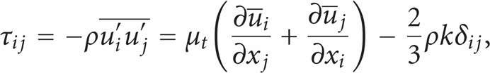
in which μ _t is the turbulent viscosity, $k(=\overline{u_i^{\prime }{u}_i^{\prime }}/2)$ is the turbulent kinetic energy, and δ _i,j is the Kronecker delta.

In determining μ _t in (4), various turbulence models in computational fluid dynamics have so far been used [19, 20]. In the present computations, the standard $k-\epsilon$ turbulence model was used [21]. This model expresses the turbulent viscosity in terms of turbulent kinetic energy, k, and its dissipation rate, ε, as

$\begin{array}{}{\mu }_t=\rho C_{\mu }\frac{k^{\mathrm{2}}}{\epsilon }.\end{array}$

(5)

In (5), C _μ is the turbulence constant that has a value of 0.09. In the $k-\epsilon$ model, the following two transport partial differential equations were solved for the values of k and ε, respectively:

$\begin{array}{c}\rho \stackrel{-}{u}\frac{\partial k}{\partial x}+\rho \stackrel{-}{v}\frac{\partial k}{\partial y}+\rho \frac{\partial k}{\partial t}=\frac{\partial }{\partial x}\left[\left(\mu +\frac{{\mu }_t}{{\sigma }_k}\right)\frac{\partial k}{\partial x}\right]+\frac{\partial }{\partial y}\left[\left(\mu +\frac{{\mu }_t}{{\sigma }_k}\right)\frac{\partial k}{\partial y}\right]+{\mu }_{t}G-\rho \epsilon ,\rho \stackrel{-}{u}\frac{\partial \epsilon }{\partial x}+\rho \stackrel{-}{v}\frac{\partial \epsilon }{\partial y}+\rho \frac{\partial \epsilon }{\partial t}=\frac{\partial }{\partial x}\left[\left(\mu +\frac{{\mu }_t}{{\sigma }_{\epsilon }}\right)\frac{\partial \epsilon }{\partial x}\right]+\frac{\partial }{\partial y}\left[\left(\mu +\frac{{\mu }_t}{{\sigma }_{\epsilon }}\right)\frac{\partial \epsilon }{\partial y}\right]\hspace{1em}+C_{\mathrm{1}}{\mu }_t\frac{\epsilon }{k}G-C_{\mathrm{2}}\rho \frac{{\epsilon }^{\mathrm{2}}}{k},\end{array}$

(6)

where G, which represents the generation of turbulent kinetic energy, is defined by

$\begin{array}{}G=2\left[{\left(\frac{\partial \stackrel{-}{u}}{\partial x}\right)}^2+{\left(\frac{\partial \stackrel{-}{v}}{\partial y}\right)}^2\right]+{\left(\frac{\partial \stackrel{-}{u}}{\partial y}+\frac{\partial \stackrel{-}{v}}{\partial x}\right)}^2\end{array}$

(7)

and $C_1=1.44,C_2=1.92,{\sigma }_k=1.0$ , and σ _ε = 1.3.

3.2. Near Wall Treatment

The standard $k-\epsilon$ model, which is the first and the most widely used two-equation turbulence closure model, has been applied to many types of flow with varying degrees of success. Unfortunately, it is insensitive to adverse pressure gradients and this causes a serious limitation to its general utility. The standard $k-\epsilon$ model avoids the integration of model equations through to the wall where the viscosity effects have to be taken into account. There are two approaches for modeling the near wall region: wall function and two-layer approach. In the wall function approach, the viscosity-affected region (i.e., viscous sublayer and buffer layer) is not solved and a semiempirical function called wall function is used to bridge the viscosity-affected region between the wall and fully turbulent region. The application of wall functions may significantly reduce both the processing and storage requirements of a numerical model. The application of the wall functions leads (provided that the grid is not too coarse) to reasonably accurate results for attached boundary layers. However, the use of wall functions becomes highly questionable for separated flows [22]. In two-layer approach, the turbulence models are modified to resolve the viscosity-affected region by extremely fine grids with no slip condition and a damping functions to account for viscous effects near the wall.

In the $k-\epsilon$ modeling of the present computations, a sufficiently fine mesh was used in simulating the near-wall viscosity-affected region with no-slip condition and the damping function presented by van Driest [23]. Based on the experimental data, van Driest [23] proposed that the mixing length, $\ell =\kappa y$ , should be multiplied by a damping function:

$\begin{array}{}{f}_{\mu }=1-\exp \left(-\frac{y^{+}}{A}\right),\end{array}$

(8)

where $y^{+}=v\ast y/\nu$ is the dimensionless distance, and the Kármán's constant κ = 0.4 and the constant A = 26. van Driest modification given by (8) improves the predictive accuracy by asymptotic description of the mixing length in the limit $y\to 0$ [18]. Using (8), the behaviors of the mixing length and the turbulence stress are described as $\ell \sim y^2$ and ${\tau }_{xy}^{\prime }\sim y^2$ , respectively, as $y\to 0$ .

3.3. Numerical Solution

Numerical solution of (1)–(3) for the unknown variables $\stackrel{-}{u}$ , $\stackrel{-}{v}$ , and $\stackrel{-}{p}$ were carried out using the finite element method (FEM). In the finite element discretization, the conservation forms, that is, the transport equations of the governing equations were used. These equations for a transferable fluid property ϕ defined per unit mass in a unit control volume read

$\begin{array}{}\frac{\partial \left(\rho \varphi \right)}{\partial t}+\mathrm{div}\left(\rho \varphi \overrightarrow{V}\right)=\mathrm{div}\left({\mathrm{\Gamma }}_{\varphi }\text{grad}\varphi \right)+S_{\varphi }\end{array}$

(9)

in which $\overrightarrow{V}$ is the velocity vector, ${\mathrm{\Gamma }}_{\varphi }$ is the generalized diffusion coefficient, and S _ϕ is the generalized source term. The fluid property ϕ takes values of 1 and $\overrightarrow{V}$ for the conservation of mass and momentum, respectively.

The discretization process consists of deriving the element matrices to put together the matrix equation as

$\begin{array}{}\left(\left[A_e^{\text{transient}}\right]+\left[A_e^{\text{advection}}\right]+\left[A_e^{\text{diffusion}}\right]\right)\left\{{\varphi }_e\right\}=\left\{S_e^{\varphi }\right\}.\end{array}$

(10)

Galerkin's method of weighted residuals is used to form the element integrals. Petrov-Galerkin approach of second-order accurate was used to discretize the advection term in the momentum equations. The time integration of the governing equations was carried out using the backward difference method. The convergence criterion for the computations of the velocity components u and v was assumed 10⁻⁶.

3.4. Solution Domain, Boundary, and Initial Conditions

The 2D solution domain for the numerical analyses of the gate flow is shown in Figure 2. The origin of the Cartesian coordinate system, $(x,y)$ , was located at the bottom left corner of the solution domain. The air-filled upper boundary was taken some distance above the free-surface of the subcritical upstream flow, and the lower boundary was the solid channel bed. The vertical gate was located at a distance x = 218 mm. No-slip boundary condition was invoked by specifying the velocity components to be zero at the fluid-wall interface, that is, at the lower boundary and on the gate surfaces, the velocity components in x and y directions were taken as $u=v=0$ . At the inflow boundary, the horizontal velocities, u, were specified as the measured velocity profile, and the vertical velocity, v = 0. The outflow boundary of the computational domain was the supercritical free overfall at the end of the channel where p = 0.

Figure 2:

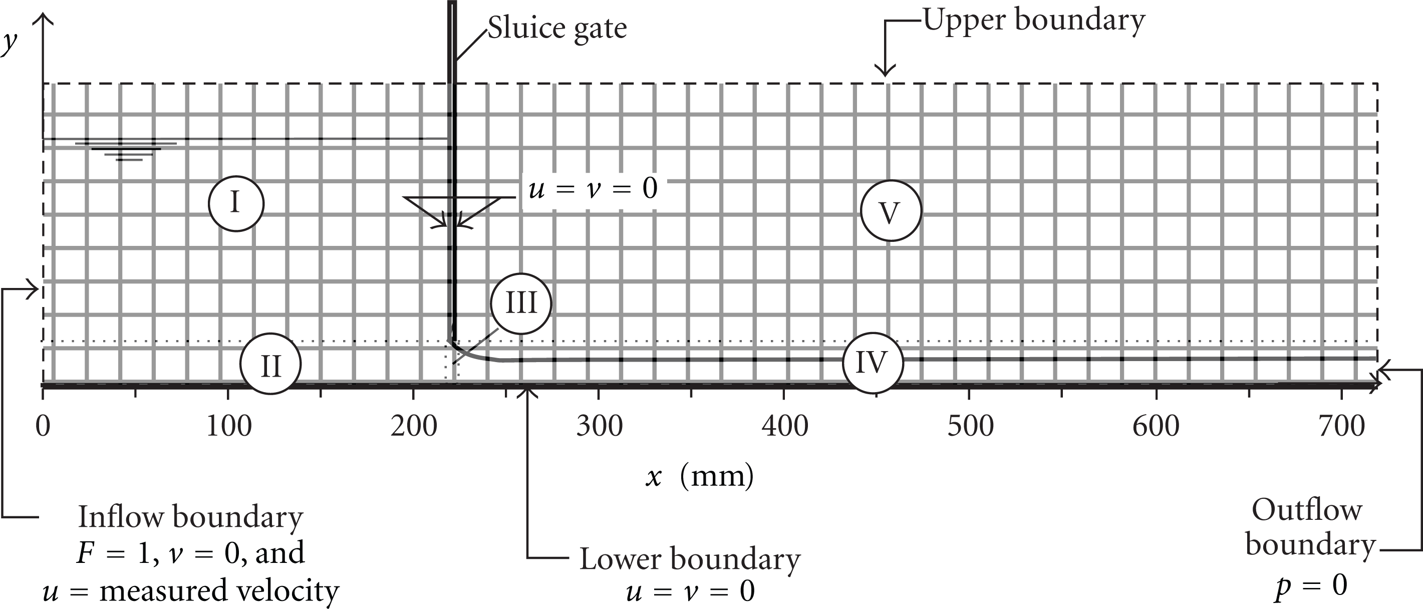
Geometry and boundary conditions of the solution domain for the gate flow.

The time-dependent solution procedure was started with the initial condition that at the inflow boundary F = 1, and continued with a time step of 0.01 s which was found suitable to speed up the convergence.

3.5. Volume of Fluid Method for Free-Surface Modeling

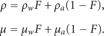
In the computation of free-surface flows, a method called volume of fluid (VOF) which is based on a concept of a fractional volume of fluid, whereby the shape and location of the constant-pressure free-surface boundary are determined successfully [4, 6, 11]. On general fixed meshes, this method uses a filling process which determines which cell in the meshing volume is filled and which is emptied [2]. Consider an Eulerian structured fixed mesh and an actual curved free liquid surface of a 2D flow field cutting through it. Then, one can define a volume fraction $(F)$ field in this mesh that can take values between 1 and 0. That is the value of F is 1 when the cell of the meshing volume is filled with liquid and is equal to 0 when it is emptied. A value of F between 0 and 1 means a fractional fill that is the free-surface lies in the cell. When $0<F<1$ , the fluid properties ρ and μ in the transport equations are calculated as the volume-fraction averaged values of water (ρ _w ) and air (ρ _a ) as follows:

$\begin{array}{c}\rho ={\rho }_{w}F+{\rho }_a\left(1-F\right),\mu ={\mu }_{w}F+{\mu }_a\left(1-F\right).\end{array}$

(11)

The time-dependent computational scheme of the VOF method proceeds as follows. At some moment in time on a finite mesh, a unique volume fraction field, F, of the water phase is calculated for a given interface and then the velocity field of the flow is obtained from the governing equations, and at the next time step, the new F field (i.e., the advected volume fraction field) is calculated and the reconstruction and orientation of the new interface is determined. For the new free-surface position the velocity field is obtained from the governing equations. The advection equation of the volume fraction is given by

$\begin{array}{}\frac{\partial F}{\partial t}+\overrightarrow{\nabla }·\left(\overrightarrow{V}F\right)=0.\end{array}$

(12)

The evolution of the free-surface in the time-dependent computational scheme is herein accomplished using an algorithm so-called Computational Lagrangian-Eulerian Advection Remap (CLEAR-VOF) which is detailed in Ashgriz et al. [5]. This algorithm utilizes exact geometric tools with no special requirement on the mesh topology, the aspect ratio, or the mesh orientation. CLEAR-VOF algorithm is based on an approach for the computation of the fluxes of fluid originating from a certain element toward each of its neighboring elements during the advection process to find out how much of fluid remains in the element, and how much of it passes into each of the neighboring cells. From an initial interface and corresponding F field, the advected polygonal shape of the free-surface, after a time step, is identified through a Lagrangian local motion using the velocities at its vertices, and the new values for the local F field of the advected liquid domain for the original Eulerian fixed mesh is determined. At the next stage, F field of the cells of the fixed mesh is redistributed and corrected so that the conservation of mass is satisfied. The corrected new F field serves as input to the interface reconstruction of the VOF code and to the flow solver for the next time step. Computation of free-surface profile by the VOF method, and the numerical solution of (1)–(3) for the 2D sluice gate flow were carried out using the software called ANSYS 10.0 which contains a general-purpose CFD package based on the FEM.

3.6. Computational Meshing

3.6.1. Mesh Design

The results of the preliminary computations showed that in order to increase the computational accuracy, the density of mesh should be changed locally as appropriate. Accordingly, taking into account the basic features of the present subcritical and supercritical flow fields upstream and downstream of the gate, the computational domain given in Figure 2 is divided into five local subdomains in which different mesh concentrations were tested. Uniform rectangular meshes were structured in all the subdomains. In constructing the computational mesh, relatively finer meshes in y-direction were used in the near-wall regions and in the region of rapid variation of free-surface profile in the contraction region of flow just after the gate (i.e., in regions II, III, and IV in Figure 2). In accordance with above considerations, three different meshes given in Figure 3 were constructed for the computations. The sizes of the mesh elements for each subdomain are given on the Figure. As may be seen in Figure 3, the differences between the three meshes are implemented in subdomains II, III, and IV only, where the vertical dimensions of the mesh elements are $\mathrm{\Delta }y=1$ , 0.5, and 0.25 mm for Mesh 1, Mesh 2, and Mesh 3, respectively. The horizontal dimensions of the mesh elements were kept constant for all three meshes as $\mathrm{\Delta }x=4$ mm for the subdomains I, II, IV, and V, and $\mathrm{\Delta }x=1$ mm for the subdomain III below the gate.

Figure 3:

Three computational meshes used in the numerical model.

3.6.2. Estimation of Discretization Error

A grid convergence index (GCI) proposed by Roache [24] was determined for the verification of computed velocities using the three mesh system described above. According to this technique, for the quantification of the discretization uncertainty of the numerical results, the fine-grid convergence index is defined as

$\begin{array}{}\text{GC}{\text{I}}_{\mathrm{23}}^{\text{fine}}=\frac{1.25\left|E_{23}\right|}{r_{23}^P-1},\end{array}$

(13)

where $E_{23}=(u_{s3}-u_{s2})/u_{s3}=$ approximate relative error between the medium and fine meshes, $u_{s2}$ and $u_{s3}=$ medium and fine mesh solutions for velocities obtained with grid spacing d₂ and d₃, respectively, and $P=\text{local}$ order of accuracy. For the three-grid solutions, P is obtained by solving the following equation:

$\begin{array}{}P=\frac{1}{\ln r_{23}}\ln \frac{\left(r_{23}^P-1\right)e_{12}}{\left(r_{12}^P-1\right)e_{23}}\end{array}$

(14)

in which $e_{12}=u_{s1}-u_{s2}$ , $e_{23}=u_{s2}-u_{s3}$ , and $r_{12}=d_1/d_2$ and $r_{23}=d_2/d_3=$ grid refinement factors between coarse and medium, and medium and fine grid, respectively. For the present three-grid comparisons the grid spacing have the following order, $d_3<d_2<d_1$ .

In this study, the profiles of the computed horizontal velocities of supercritical flow at $x=0.24$ m, just downstream of the sluice gate, were used to determine the numerical uncertainties due to discretization (Table 2). In the assessment of GCI values in (13), the average order of accuracy, $P=P_{\text{ave}}$ , over the flow section was used. It is seen that the maximum discretization uncertainty in the chosen velocity profile (with 16 number of points) for the fine-grid solutions on Mesh 3 is $0.73\%$ corresponding to $\pm 0.0070$ m/s which remains within $2\%$ and shows an excellent indication for a mesh-independent solution.

Table 2:

Discretization error estimate in velocity profile at x = 0.24 m.

Quantity	Error estimates in velocity
Number of points	16
$P_{\min }$ , $P_{\max }$ , Pave	0.43, 6.97, 2.28
Max ${\text{GCI}}_{23}^{\text{fine}}$	0.73% (±0.0070 m/s)

4. Experimental and Numerical Results

In the following, the numerical results for the velocity field and free-surface profile from the VOF-based CFD modeling of 2D rectangular open channel flow under a vertical sluice gate are presented. The results of the numerical simulation obtained from the three meshes given in Figure 3 are compared with experimental results, and the sensitivity of the numerical model to the computational meshing is discussed. It is generally accepted that very near the wall from no-slip at the wall to about $y^{+}=v\ast y/\nu \approx 30$ , turbulence is damped out and the boundary layer is dominated by viscous shear [19], where $v_{\ast }={({\tau }_0/\rho )}^{1/2}$ is shear velocity and τ₀ is boundary shear stress. In the present computational results of all three meshes, the values of y⁺ remain within 30 for $x\le 205$ mm. That means, up to a location very close to the wall, the flow in the near-wall elements is treated as viscous in character.

4.1. Comparison of Computed and Measured Velocities

From the PIV measurements of flow velocities, the vertical distributions of the horizontal velocity components at different locations upstream of the vertical gate are given in Figure 4. The vertical distribution of horizontal velocities at x = 0 is used as the inflow boundary condition for the numerical computations. The horizontal velocity profile at x = 193 mm corresponds to the Reynolds ridge position on the water surface, where the horizontal velocity is zero. The ridge position which is characterized as the plunging point of the stagnation flow behind the vertical gate has a horizontal distance of L _R = 25 mm from the gate for the present experimental conditions.

Figure 4:

Experimental horizontal velocity profiles at various locations upstream of the gate.

Vertical distributions of experimental and numerical results of dimensionless horizontal velocities, $u/V_0$ , at locations of $x=38,80,119,161$ , and 204 mm for the three meshes are given in Figure 5. From the comparisons of the velocity distributions, it is seen that the computational results from Mesh 1, Mesh 2, and Mesh 3 are very close to each other and in general they show reasonable agreement with experimental velocity distributions. The disagreement between the results of numerical model and experiment in Figure 5 seems to slightly increase toward the free-surface in part of the solution domain where $x\le 80$ mm, in that region Mesh 3 is the most successful.

Figure 5:

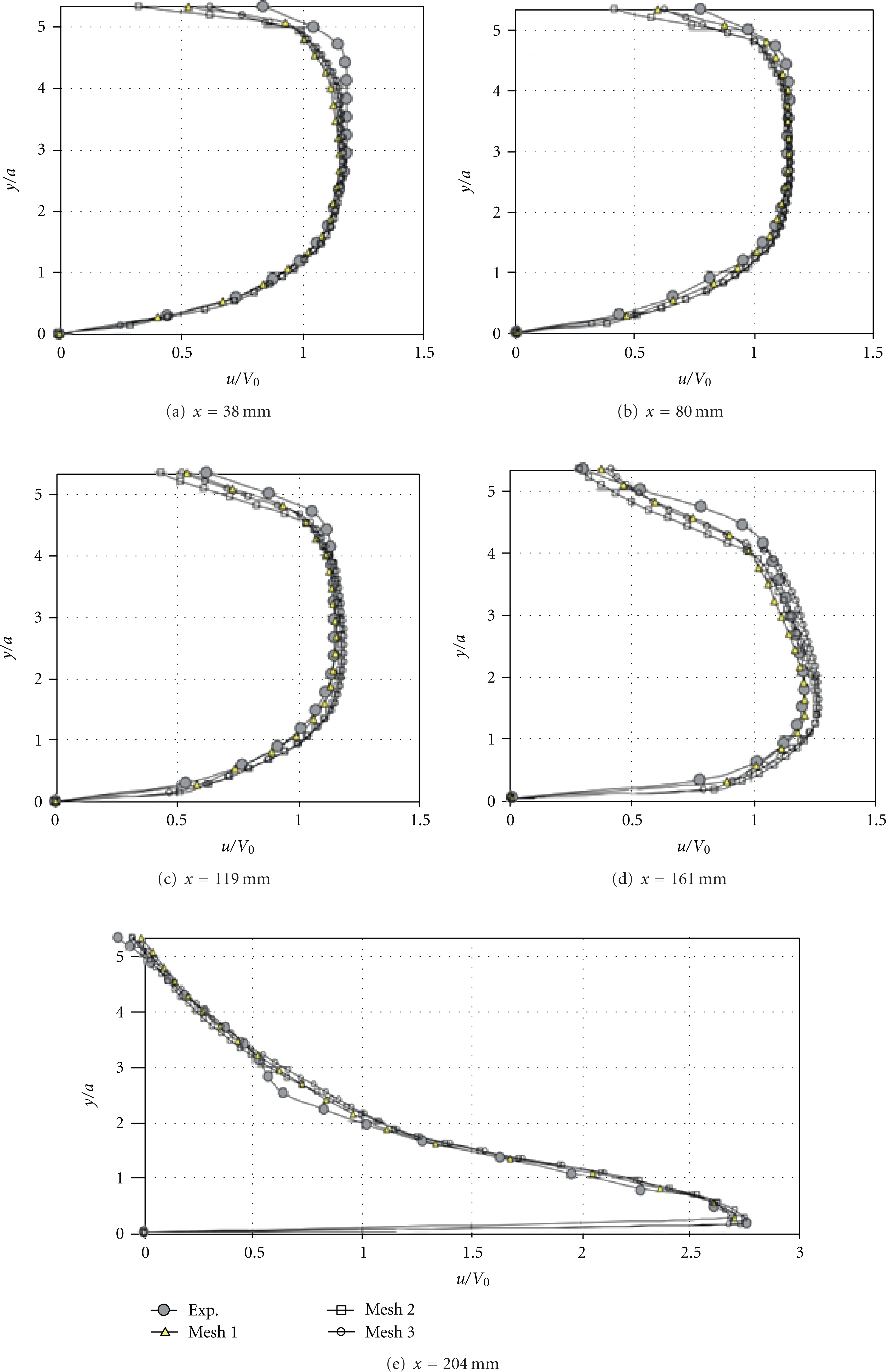
Comparison of experimental and computed horizontal velocity profiles for three meshes.

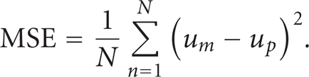
For a quantitative evaluation of the comparison of the experimental (u _m ) and predicted (u _p ) velocities, the mean square error (MSE) is calculated at section x = 204 mm. The MSE is given as

$\begin{array}{}\text{MSE}=\frac{\mathrm{1}}{N}{\sum }_{n=\mathrm{1}}^N{\left(u_m-u_p\right)}^{\mathrm{2}}.\end{array}$

(15)

The MSE values are found as 0.00210, 0.00196, and 0.00174 for Mesh 1, Mesh 2 and Mesh 3, respectively. That means the predicted accuracy of the simulation regarding the flow velocity is the best for Mesh 3.

Figure 6 shows the vertical distributions of measured and computed dimensionless vertical flow velocities, $v/V_0$ , at the two sections $x=193$ mm and 204 mm, close to the gate from the three meshes. The vertical velocity comparisons show generally good agreement between the results of numerical model from the three meshes and experiment. However Figure 6 clearly demonstrates that the computed results produced by Mesh 3 are relatively better over the entire flow depths.

Figure 6:

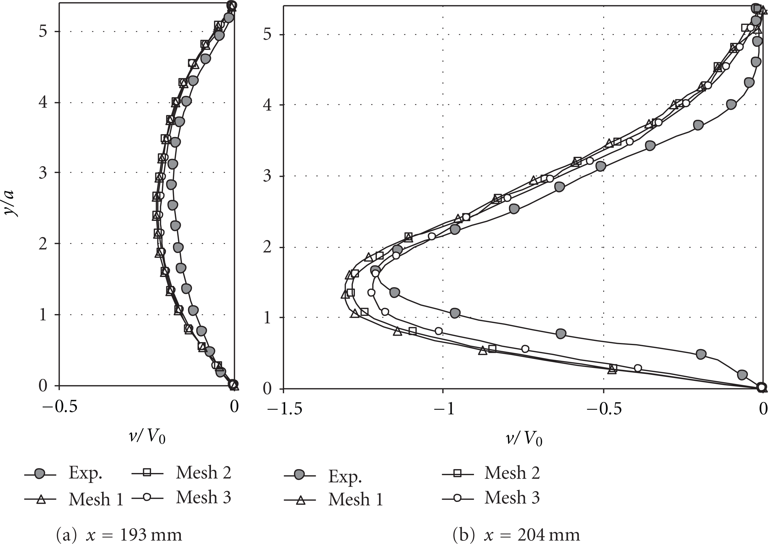
Comparison of experimental and computed vertical velocities for three meshes.

From the examination of the velocity distributions given in Figures 5 and 6, it is difficult to detect a very distinct effect of mesh density on the computed velocities throughout the solution domain. Since the increasing of the mesh concentration does not result so much improvement on the computed velocities, and besides considering the advantage of shorter computing time, Mesh 1, that is the coarsest of the three meshes, can be used to adequately describe the computed velocity field for the flow region upstream of the gate. Actually, a reasonable investigation into the mesh density effect on the flow properties must also include the problem of accurate prediction of flow profile which will be discussed in the following section.

Figure 7 gives the measured and computed velocity vector fields upstream of the gate using Mesh 3. It is seen that experimental and computed velocity fields display a clear zone of swirling motion, called the recirculation region, behind the gate where the water in the surface flows in reverse direction. The ridge position on the water surface can be detected from the velocity vector field.

Figure 7:

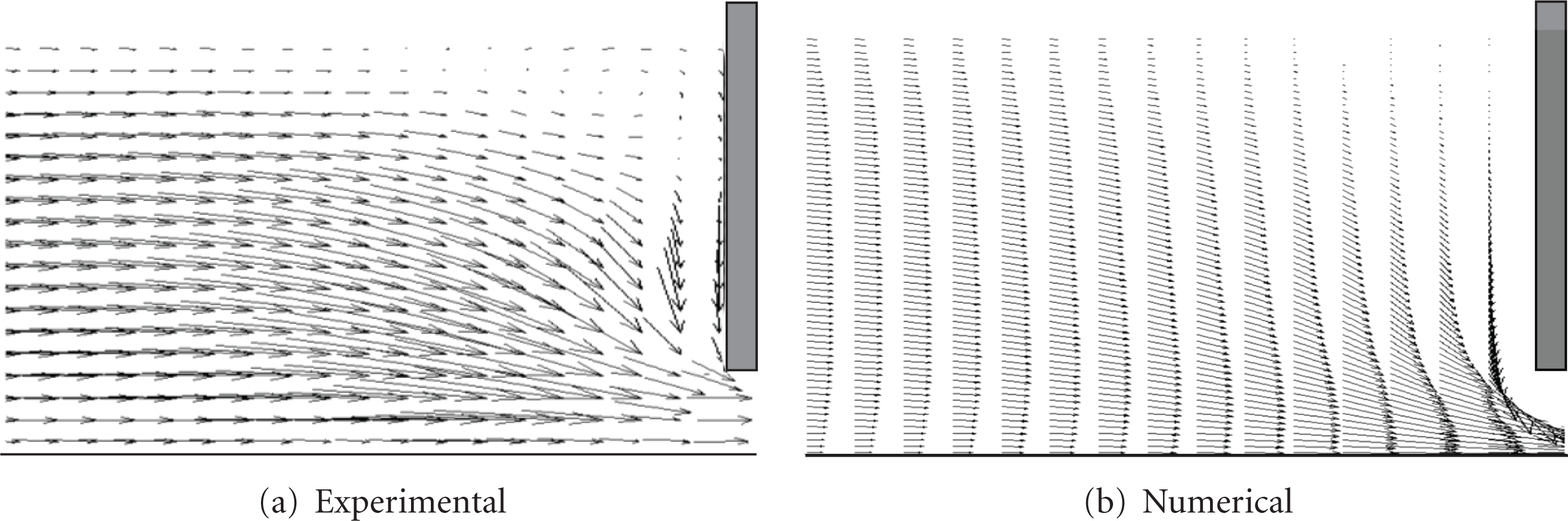
Measured and computed velocity vector fields upstream of the gate using Mesh 3.

4.2. Comparison of Computed and Measured Flow Profiles

Figure 8 shows the computed and measured subcritical flow profiles upstream of the gate from the three meshes. It is seen that the computational upstream flow profiles are almost similar for the three different meshes. From the computations using the three meshes, the upstream flow depths were all found as $h_0=66$ mm which is slightly higher than the measured depth of 64 mm.

Figure 8:

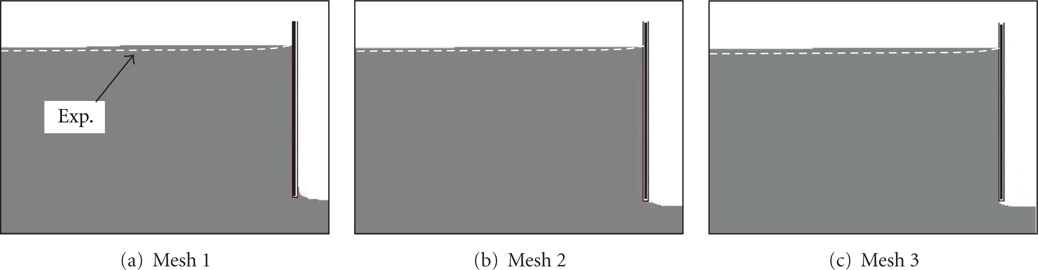
Computed and measured flow profiles just upstream of the gate for three meshes.

The supercritical downstream flow contains a rapidly varied profile between the gate outlet and the contraction section. Because there is a considerable change of flow depth along the rapidly varied contraction region, regarding the mesh effect, this portion of the flow within the solution domain is considered as the most decisive in comparing the computed and measured flow profiles. Computed flow profiles in the rapidly varied contraction region under the gate and the values of the contraction coefficient, C _c , obtained from the three meshes are given in Figure 9. From the examination of the three computed profiles in Figure 9, it is seen that in contrast to the velocity distributions presented in Figures 5 and 6, the shape of the flow profile and the value of contraction coefficient are very sensitive to the mesh refinement. Figure 9 clearly shows that the refinement of the mesh in vertical direction has improving effect on the flow profile. Regarding the physical appearance of the computed profiles in Figure 9, Mesh 1 produces a contraction profile which is far from the real occurrence. On the other hand, Mesh 3 seems to give the most realistic surface profile with contraction coefficient of C _c = 0.71, and contraction length of L _c = 14.8 mm, these two quantities are quite in agreement with the experimental values of 0.69 and 14 mm, respectively. From the computed flow profiles in Figure 9, Mesh 3 appears to be the most suitable of the three meshes in predicting the flow profile in the contraction region under the gate.

Figure 9:

Computed flow profiles in the rapidly varied contraction region under the gate for three meshes.

During the running process of the VOF analysis, the development of the computational free-surface profile within the solution domain, using Mesh 3, is given in Figure 10. According to the VOF analysis, the time dependent filling process of the solution domain is demonstrated through Figures 10(a) to 10(f). As may be seen in Figures 10(e) and 10(f), the flow profiles are almost identical at times t = 13 s and 15 s, that means the filling process of the solution domain is completed and the computed free-surface development is stabilized at t = 13 s. It is seen in Figure 10(e) that the final shape of the computed flow profile displayed within the solution domain is well in agreement with the experimental profile.

Figure 10:

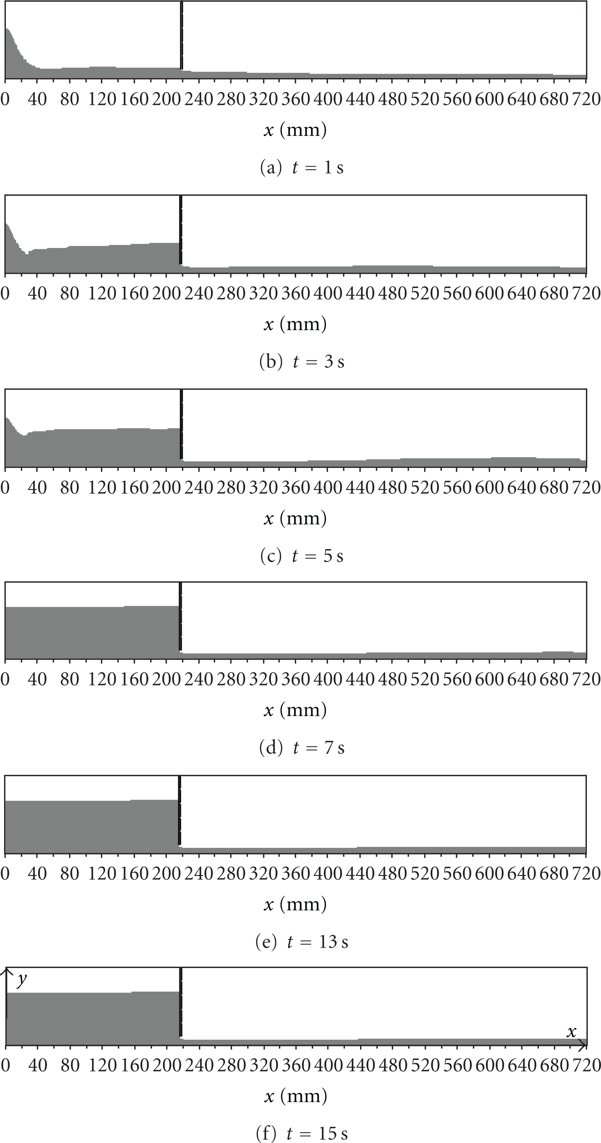
Development of the computed free-surface profile using Mesh 3.

From the comparisons of the computed and experimental results discussed above, Mesh 3 among the three computational meshes given in Figure 3(c) may be suggested as the most suitable mesh construction in predicting both the velocity field and the free-surface profile of the present flow case.

The present numerical simulation is based on the 2D analysis of the flow which ignores the side wall effect on the mid-span of the channel. It is widely accepted that this case is realized when the aspect ratio of the flow section is greater than 5. This condition is presently well satisfied in the supercritical flow downstream of the gate. In the subcritical upstream region the aspect ratio is 3.125 which is less than 5. However with the existing aspect ratio and considering the level of Reynolds number for the upstream flow, it is expected that the results of the present 2D analysis have acceptable numerical accuracies.

5. Conclusions

Experimental and numerical study of 2D open channel flow under a vertical sluice gate is carried out. Using the standard $k-\epsilon$ turbulence model, the governing equations of the flow are solved by finite element method. In the numerical simulation, the VOF method is used to determine the flow profile. Experimental and computed velocities and free-surface profiles from three different meshes are presented. A grid convergence analysis is carried out for the verification of computed velocities. Mesh density is relatively increased in the lower part of the flow which comprises the boundary layer of the upstream flow and supercritical downstream flow where rapid variation of the surface profile occurs. In the lower part of the computational domain, different mesh densities in y-direction for each one of the three meshes are used to determine the sensitivity of computed results to the meshing of solution domain. From the comparisons of experimental and numerical results of three structured meshes used in the present computations, it is found that the computed flow profile is much more sensitive to the refinement of the mesh than the computed velocity field. That means in regions where flow profile changes rapidly, the mesh construction must be given special attention to design the mesh refinement in vertical direction. Based on the comparisons of experimental and numerical results of this study, it may be concluded that the VOF-based CFD modeling can successfully be used to analyze the 2D open channel flows which interact with vertical sluice gates, provided that suitable computational mesh is constructed.