
Abstract
The needs of diverse environmental information introduce the multimedia data into wireless sensor networks. The characteristics of most multimedia information, such as great amounts of data and high-quality requirement for network service, positively affect traditional wireless sensor networks, which also derive various new research areas. This paper focuses on the multimedia image sensor networks and proposes FVPTR (fuzzy image recognition and virtual-potential-field-based paired tangent point repulsion) method to enhance the perspective coverage of network. This approach utilizes fuzzy image recognition method to process the boundary nodes. Aimed at nonboundary nodes, based on potential field theory, it adopts paired tangent point repulsion mechanism, which attempts to obtain the optimal network sensing coverage through the multiple paired achievements between one current node and several target nodes. Combined with FVPTR, some algorithms such as LRBA, MBAA, and mixed superposition algorithm are put forward to single or multiple-time adjustment by the rotation of the direction angle. The results of simulation and all kinds of comparisons show that three-times pairing method enhances the coverage of networks well.
1. Introduction
Wireless senor networks (WSNs) enjoy great applications in traditional fields such as industry, agriculture, military, and environmental monitor. Besides, WSNs also show the superiority in areas of household paradigm, health care, transportation, and so forth. With the occurrence of new applications, the needs for diverse environmental information from users are increasing, and the multimedia information is introduced into wireless sensor networks. The characteristics of most multimedia information, such as amounts of data and high-quality requirement for network service, greatly affect the traditional techniques of WSNs and meanwhile derive some new research points. Deployment and coverage are two typical issues, which not only reflect the perceptive ability of networks to physical world, but also are directly related to the quality of network services [1].
Numerous researches have focused on the coverage issues [2–7]. Jing and Alhussein [5] gave out a coverage model of target points for direction sensor, proposing LPI algorithm to compare with CGA and DGA algorithms. Judging from the simulation results, it could not show significance in coverage enhancement, and it was a preliminary study on directional sensors. Tao et al. [8] changed the coverage-enhancing problem into virtual-potential-field-based centroid points' uniform distribution problem which ignored the effect of border nodes. Mohamed and Hossien [6] proposed PCP protocol based on omnidirectional image sensors and deduced several models, in which the exponential model is an inspiration for our method. Zou and Krishnendu [9] used VFA algorithm to generate the mobile paths for sensor nodes based on virtual potential field and artificially changed the location of each node in accordance with the calculated trajectory. Nonetheless, it is almost impossible to achieve in the case of large-scale deployment.
Image sensor is a typical case of directional sensors. This paper discusses the scenario that stochastically deployed image sensors in limited areas and uses paired tangent point repulsion method based on fuzzy image recognition and virtual potential field theory to improve the coverage of image sensor networks.
2. Preliminary
2.1. Fuzzy Image Recognition
Oztarak et al. [10] demonstrated that image sensors could perceive “video event” once accessing into field of view (FOV) [5, 11]. He utilized joint fuzzy processing method with micro-SEBM (structural and event based multimodal) to compose the mobile trace of “video event” in an image captured by nodes and demonstrated that image sensors had the ability to identify the “video event.” Then the specific location of “video event” would be positioned in the current image through scanning it and be clearly expressed by MBR (minimum bounding rectangle) information which could be recorded for further operation.
The frequency and the amounts of data of most monitors and household cameras cannot be afforded by wireless multimedia sensor networks (WMSNs). A specific image sensor node developed according to actual demand would be used as the hardware to test the fuzzy image recognition method in the following experiments.
The node as shown in Figure 1 is equipped with ATmega128 processor, OV7620 image processing chip, and CC2420 communication chip. Moreover, it can work at two modes of 24-bit color and 8-bit grayscale, and sample images at three different pixel resolution ratios such as 88 * 72, 160 * 120, and 320 * 240.

Photos of point light source at 100 m, 200 m, and 300 m away from the image sensor node.
The flashlight with AA battery is used as point light source in this experiment. The node working at the mode of 24-bit color and the pixel of 160 * 120 takes photographs on the point light source, as shown in Figure 1.
The image sensor node scans the data of photo. It has not distinguished the point light source until scanning the Xth line and the Yth column and then records the value of column in an array named D until the light source disappears from the Xth line. When scanning the (X + K)th line, the same operation would be done until the node finishes scanning the whole image. After calculating the average value of D, the average column value (ACV) of “video event” in the current image can be figured out. The specific application of ACV will be described in Section 4.1.
2.2. Directional Sensing Model
In Figure 2, the effective sensing area of directional sensor is fan-shaped region of OAB which can rotate around the point O. The perceptive radius of directional sensor is R, which will be depicted in Section 2.3.

Directional sensing model.
At a discrete moment, it can be determined whether any point P is covered by a directional node or not by the following:
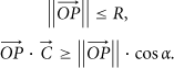
If a point P meets the above two conditions simultaneously, it is covered.
There are two concepts that should be distinguished well.
(1) “Effective sensing area”: fan-shaped region of OAB shown in Figure 2 can be calculated by measure of area.
(2) “FOV”: sensor's field of view is the angle of effective sensing area and can be depicted by the dimension of angle.
2.3. Perceptive Radius Theory
Here, two conceptions of perceptive radius are proposed.
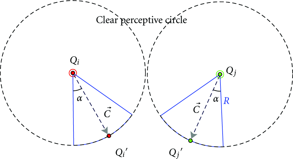
(1) “Radius of clear perception”: in range of this radius, an image sensor node can clearly identify any object accessing into its FOV. The scope of clear perceptive radius is [0, R]. The perceptive ability of an image sensor remains constant in the range of clear perceptive radius as shown in Figure 3.

Perceptive ability and perceptive radius.
(2) “Radius of fuzzy perception”: in range of this radius, an image sensor node cannot clearly identify the object accessing into its FOV. The requirements of environmental monitoring cannot be well met, but the node can respond to special “video event.” Strong light source is such a typical case of special “video event.” The scope of fuzzy perceptive radius is
One case is presented as follows: there is an image sensor at the starting point of O. Meanwhile, a strong light source is set at an infinite distance away from starting point as shown in Figure 4. The light source lies in the range of the node's fuzzy perceptive radius. The sensor cannot clearly identify the targets near the light source, that is, it also cannot monitor the environment there. But the “video event” of strong light source can be perceived just as the experiment described in Section 2.1.
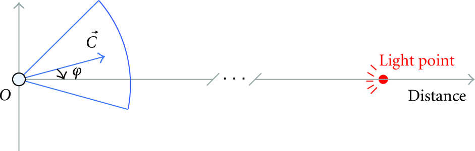
Image sensor node and sensing light source.
The angle between
2.4. Virtual Potential Field
Introducing virtual potential field into WSNs originates from its application in obstacle avoidance [12, 13]. Virtual potential field, due to the simplicity and the characteristic of real time, has been introduced into the coverage problem in WMSNs [8]. In virtual potential field, each node can be considered as a virtual charge, suffers the virtual force from other nearby nodes, and gets the trend of moving towards the region of less node density in networks.
Tao et al. [8] figured out that the focus of each sensor node's effective sensing area would rotate around the node while suffering virtual force from neighboring nodes. Resultant force from all neighboring nodes within the scope of effective communication should be taken into account, which inevitably increased the difficulty of force analysis and the complexity of algorithm. So before FVPTR is executed, the process of pairing between two adjacent nodes should be achieved. The proposed method ignores the influence of most nearby nodes, only focusing on adjusting the two paired nodes' perceptive direction angles in terms of the virtual force between them as reducing the complexity of computation as possible. Moreover, the simulation results prove that FVPTR indeed enhances the perspective coverage of networks.
3. Framework
The fuzzy image recognition and virtual potential field methods are specifically introduced in this section.
3.1. Initialization
Image sensor nodes are randomly and uniformly distributed in a monitored region. Some typical coverage enhancing algorithms often assume that nodes can estimate their locations. Equipping every node with GPS will bring some of the cost, so localization is typically performed by estimating distances between neighboring nodes. In this paper, we focus on application in which localization is unnecessary and possibly infeasible. So we consider that nodes are unaware of their locations.
Strong light source, that causes the “video event,” is set in the center of each boundary in the region. Unfortunately, the coverage of networks is unsatisfactory after initial deployment, and there exists large amounts of “overlapped regions.” “Overlapped region” can be defined as a region that is covered by more than two nodes effective sensing area at the same time.
In fact, how to enhance the coverage and reduce the “overlapped region” has already been the same issue in this paper.
3.2. Virtual Force
The potential field is a model of electrostatic field in physics. Each node can be seen as a point charge in the electrostatic field and has the same energy. In other words, these nodes are identical with the same type of charge and the same equivalent electricity. Taking into account the nature of the homosexual repulsion and heterosexual attraction, it is reasonable to suppose that the virtual force in this potential field is repulsion between two homogeneous nodes. But the repulsion is different from general repulsion between charges.
There are two image sensor nodes, whose clear perceptive radius is R, named as
Nearby unpaired nodes.
Not only the data quantity of WMSNs is larger than that of normal WSNs, but also the integrity of multimedia data is more important than that of scalar sensing data. In order to ensure the quality of communication while avoiding frequent data loss or interruption, reducing the actual distance between nodes becomes a valid method.
Effective communication radius of one node marked with
The Euclidean distance between
“Paired nodes” is a pair of nearby nodes,
As shown in Figure 6, the repulsion between two nodes should be considered when


Force analysis of paired nodes.
The repulsion from
In order to move the force point without changing the direction and the value of force, we suppose that
The perceptive directions of nodes belong to uniform distribution after initial deployment. Hence, there might be some special situations, for example, when
In practice, the value of RSSI (received signal strength indicator) [14, 15] can be used to determine the nearest node away from the current node. The two paired nodes have to interchange messages to inform each other the distance and perceptive direction information. If both
3.3. Perceptive Direction Adjustment
Because of the virtual force between two paired nodes, adjustment of angular magnitude turns out to be a trouble in coverage problem. We propose two calculating methods, that is, one is linear-relation-based algorithm and the other is a mechanism-based approximate algorithm.
3.3.1. Linear-Relation-Based Algorithm (LRBA)
LRBA is used to calculate the angular magnitude marked by Δ φ that needs to be adjusted. Figure 7 is the paradigm based on LRBA.

The paradigm based on LRBA.
In Figure 7,

Equation (3) can generate the following:
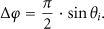
The range of
3.3.2. Mechanism-Based Approximate Algorithm (MBAA)
Because


Relationship of
The range of Δ φ is so wide that it would directly aggravate the energy consumption while adjusting perceptive direction without some constrains. So it will assume that Δt is a fixed value in an adjustment in our proposed methods, regardless of the rotation angle value is very large or very small. And (7) can be simplified into (8).
In (8), Δ
φ
is affected by
Relationship between
Equations (4) and (8) are consistent with the needs of practical application and will be elaborated in Section 4.2.
4. Implementation
4.1. Detailed Steps
The FVPTR method proposed in this paper follows steps below with the premise of the network is connected.
(I) deploy N sensors randomly in the monitored region. The sink broadcasts the hop-explored packet. After receiving it, each sensor node records the hop information and adds one to current hop value then rewrites the packet and sends it out. Finally, each sensor node sends packet back to the sink to notify the hop information. Then the sink chooses those sensor nodes, with the largest hop value, records them as boundary nodes and sends “video event” searching command to them.
(II) sensor nodes that accept video event searching command start up video event searching algorithm. It is described as in Algorithm 1.
γ is the value of rotation;
ε
is a given tiny value;
β
is a value that is larger than
ε
(we assume that
β
=10
ε
); “M” is defined as half of the pixel width value of current image. A current captured image is scanned by the node. The node generates a random number marked with RAND in the range of [−1, +1]. } Calculate the current ACV; } The perceptive direction of node is counterclockwise adjusted for
γ
; Counterclockwise rotates for
γ
; }
Algorithm 1
(III) the nodes that do not accept video event searching command start virtual-potential-based paired repulsion algorithm as in Algorithm 2.
range of RSSI value (inversely proportional to the distance), then marks it as target node; target node. It responses the request and marks the sender as its paired node, then sends back confirmation-paired packet to the current node; so the target node becomes the paired node of current node; } The target node is in the process of pairing with other nodes; the current node will wait for the time slot of
τ
then select another target node with the second largest RSSI value and continue pairing process with reference to a. } Repeat the above procedure until the current node finds its all neighbors are paired with others or the time domain is over. { A NUMBER is generated randomly in the range of [−1, +1] by the node sent the request-paired packet. The perceptive direction is clockwise adjusted for
π
/6; Taking inverse operation to NUMBER value, the sensor obtains paired node. Then, the paired node does the same operation as follows: The perceptive direction is clockwise adjusted for
π
/6; calculates
θ
, then computes Δ
φ
according to(4) and (8) respectively;
Algorithm 2
(IV) each nonboundary node adjusts its perceptive direction in terms of Δ φ .
4.2. Remark
The result of step I can effectively distinguish boundary nodes from nonboundary nodes. No doubt that it is the foundation and prerequisite for adjusting perceptive direction of two different kinds of nodes.
Step II elaborates the whole process of video event searching algorithm. It is important for initialization, since actual testing should be done to make sure that image sensor nodes can effectively keep sensitive to “video event” such as strong light source without responding to general event.
In step III, if the current node cannot receive confirmation-paired packet from target node within the given time slot τ, it will search for another node nearby in the range of
From the perspective of optimizing overall coverage, two improved algorithms based on (4) and (8) will be further proved in Section 5.
5. Simulation
5.1. Single-Time Adjustment
The value of FOV is π /3 in line with actual test in Section 2.2, and α is π/6. N nodes are distributed in a square region of 500 m * 500 m. Their perceptive directions are subject to uniform distribution in the range of [0, 2 π ]. Different equations are used to calculate Δ φ of each node. All simulation data listed below are the average value of numerous (100 times) test results.
The results of simulation for LRBA, MBAA, and mixed superposition algorithm are shown in Table 1. The calculation on Δ
φ
of mixed superposition algorithm can be depicted as follows:
Comparison of different algorithms (
α
= π/6, R = 60 m,
Obviously the enhancement of mixed superposition algorithm seems to be better than two other methods. However, owed to the stochastic character, mixed superposition algorithm reduces the complexity of computation and the degree of enhancement.
Whatever any algorithm, single-time adjustment fails to gain enhancement more than 6%, which cannot meet the actual demands.
5.2. Multiple-Time Adjustment
After the first successful pairing, each node starts the second pairing. For each node, it neglects the node that has paired with itself in the first time and searches for another node in the range of 
It is significant for three-time adjustment to use different algorithms. In the second pairing, the current node searches for another node that has the shortest distance from it. Nonetheless, the distance should be longer than that of the first paired node from the current node, as similarly in the third adjustment. According to (2), the farther the distance between two paired nodes is, the less the force between them should be. Moreover, the less the force is, the smaller Δ φ is. So the farther the distance is, the smaller the adjusting angle value is. The relation of the average value of each algorithm's Δ φ can be arranged that LRBA in the first adjustment > MBAA in the second adjustment > mixed subtraction algorithm in the third adjustment.
We examine the effect of the number of adjustment. In the condition that α = π /6, R = 60 m, and N is set 100, 200, and 300, respectively, as shown in Figure 10, with the increase of the number of adjustment, the coverage increases linearly until the number of adjustment reaches 3 and then becomes saturated when the number of adjustment is above 3. So we assume the number of adjustment is 3 in the following simulation.

The effect of the number of adjustment.
In the condition that
α
=
π
/6, R = 60 m, and

The results of three-time adjustment.
The boundary nodes are colored with green, while nonboundary nodes are blue. The coverage of networks is enhanced evidently as shown in Figure 11(d). The detailed values are listed in Table 2.
Results of algorithm that adjusts for three times corresponding to Figure 11.

In the premise of initial deployment, coverage is 72.13%, by 100 times tests, Table 3 displays the comparative average results on adjusting for five times with the parameters
α
=
π
/4, R = 60 m, and
Average results of algorithm that adjusts for five times with other parameter values.

From Tables 2 and 3, after three adjustments, the coverage improves nearly twice that of the single-time adjustment. By actual tests, there is only little difference between the results of three-time adjustment and adjusting for more times. However, the unsatisfactory results of declining in coverage occur after adjusting for more than ten times. Because of the random feature of algorithms, the more the times of pairing are, the more difficult to control the final outcome of adjustment is.
5.3. Coverage Enhancing versus Different Parameters
Case 1 (changes in the value of “α”).
As shown in Figure 12, the enhancement gains the optimal value when α = π/4 in all of four algorithms. The worst situation occurs while α is π/3. The changes generated by diversity of α in different algorithm roughly have the same trend which turns out to be Z-shaped discipline in Figure 12.
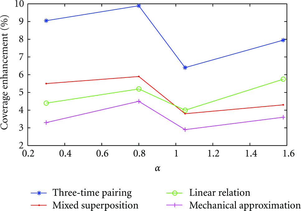
Influence on enhancement caused by α.
Case 2 (changes in the value of “N”).
Coverage comparison of different algorithms is expressed in Figure 13 through changing the number of nodes N, while α = π/6 and R = 60 m.
As shown in Figure 13, the effect on enhancement caused by different algorithms can be sorted that three-time pairing > mixed superposition > linear ration > mechanical approximation. And the following conclusions can be drawn after analyzing the data in Figure 13.
(a) Different algorithms gain different peak position. The peak of three-time pairing and mixed superposition appear in vicinity of 100 nodes while that of two others occur in vicinity of 150 nodes.
(b) In vicinity of 200 nodes, the effect of each algorithm turns out to a certain degree slow-paced.
(c) When the number of nodes is beyond 250, the coverage improvement of each algorithm gradually declines.
The reasonable explanations for those phenomena are as follows.

Influence on enhancement caused by N.
Situation A
The average values of angles that need to be adjusted of three-time pairing and mixed superposition are larger than that of two other algorithms. Meanwhile, once reaching the coverage peak value, required nodes number of three-time pairing and mixed superposition is less than lined relation and mechanical approximation. It is confirmed that there must be some relationship between the peak of enhancement and angles that need to be adjusted.
Situation B
In vicinity of 200 nodes, the NR/NC (quotient of network redundancy dividing network coverage) gains its minimum value. In other words, the network configuration resource is utilized adequately when the number of nodes is about 200. So in this situation, the outcome of adjustment is not remarkable.
Situation C
With the continuous increasing on the number of nodes in a limited area, the coverage enhancement gradually becomes saturated.
Case 3 (changes in the value of “R”).
Figure 14 shows the condition that N is 100, α is π/6, and the value of R is gradually increasing along the horizontal axis direction.
The following conclusions can be drawn.
(A) The peaks of three-time pairing and mixed Superposition occur in vicinity of 60 m while that of linear ration and mechanical approximation do in vicinity of 80 m.
(B) The changes of enhancement of four algorithms keep the same trend, which rises firstly and then falls down after reaching the peak.
(C) Except in vicinity of 80 m and 90 m, the enhancement of algorithms can be sorted that three-time pairing > mixed superposition > linear ration > mechanical approximation.
The trend of changes in Figure 14 can be understood from several aspects.

Influence on enhancement caused by R.
Situation A
Like the situation described in Figure 13, the peaks of different algorithms emerge at different positions. From the macropoint of view, the impact on coverage enhancement caused by average value of angle adjusted shows that the peak position of linear ration and mechanical approximation lags behind two other algorithms.
Situation B
When the radius of nodes tends to zero, analysis of coverage cannot be set up and coverage enhancement cannot be realized as well. When the radius tends to infinite the complete coverage can be achieved after initial deployment. In practice, the enhancement would be conspicuous only in a certain range of radius.
Situation C
As shown in Figure 14, ignoring the effect of peak value, the three-time pairing algorithm shows its advantage mainly due to taking into account the impacts of other neighboring nodes.
6. Conclusion
In this paper, based on virtual potential field, the paired tangent point repulsion for nonboundary sensor nodes and fuzzy image recognition for boundary sensor nodes realize the enhancement of perspective coverage, together with LRBA, MBAA, and mixed superposition algorithm for rotation angle adjustment. Furthermore, through simulation experiments based on the above algorithms, three-time adjustment method gains better performance than single one and more satisfactory cost-efficacy ratio than more-time adjustment method.
However, there exists defects in the algorithm execution of FVPTR, for example, some nodes could not find their respective paired partner such as those with only one neighbor or the remaining one alone from the odd numbers of total. This is the emphasis in the further research, and meanwhile coverage issue on video or audio sensors networks will be developed in the next work.
Footnotes
Acknowledgments
The subject is sponsored by the National Natural Science Foundation of China (nos. 60973139, 61003039, 61170065, and 61171053), Scientific and Technological Support Project (Industry) of Jiangsu Province (nos. BE2010197, BE2010198), Natural Science Key Fund for Colleges and Universities in Jiangsu Province (11KJA520001), the Natural Science Foundation for Higher Education Institutions of Jiangsu Province (10KJB520013, 10KJB520014), Academical Scientific Research Industrialization Promoting Project (JH2010-14), Fund of Jiangsu Provincial Key Laboratory for Computer Information Processing Technology (KJS1022), Postdoctoral Foundation (1101011B), Science and Technology Innovation Fund for Higher Education Institutions of Jiangsu Province (CXZZ11-0409), the Six Kinds of Top Talent of Jiangsu Province (2008118), Doctoral Fund of Ministry of Education of China (20103223120007, 20113223110002), and the Project Funded by the Priority Academic Program Development of Jiangsu Higher Education Institutions (yx002001).