More Benefits of Adding Sparse Random Links to Wireless Networks: Yet Another Case for Hybrid Networks

Abstract

We theoretically and experimentally analyze the process of adding sparse random links to random wireless networks modeled as a random geometric graph. While this process has been previously proposed, we are the first to prove theoretical bounds on the improvement to the graph diameter and random walk properties of the resulting graph as a function of the frequency of wires used, where this frequency is diminishingly small. In particular, given a parameter k controlling sparsity, any node has a probability of $1/k^{2}n{r}^2$ for being a wired link station. Amongst the wired link stations, we consider creating a random 3-regular graph superimposed upon the random wireless network to create model $G_1$ , and alternatively we consider a sparser model $G_2$ as well, which is a random 1-out graph of the wired links superimposed upon the random wireless network. We prove that the diameter for $G_1$ is $O\left(k+\log \hspace{0.17em}\hspace{0.17em}\left(n\right)\right)$ with high probability and the diameter for $G_2$ is $O\left(k\log \hspace{0.17em}\hspace{0.17em}\left(n\right)\right)$ with high probability, both of which exponentially improve the $\mathrm{\Theta }(\sqrt{n/\text{log}n})$ diameter of the random geometric graph around the connectivity threshold, thus also inducing small-world characteristics as the high clustering remains unchanged. Further, we theoretically demonstrate that as long as k is polylogarithmic in the network size, $G_1$ has rapidly mixing random walks with high probability, which also exponentially improves upon the mixing time of the purely wireless random geometric graph, which yields direct improvement to the performance of distributed gossip algorithms as well as normalized edge connectivity. Finally, we experimentally confirm that the algebraic connectivities of both $G_1$ and $G_2$ exhibit significant asymptotic improvement over that of the underlying random geometric graph. These results further motivate future hybrid networks and advances in the use of directional antennas.

1. Introduction

Ever since the first observation of “six degrees of separation” by Milgram [1], small-world phenomea have been noted in numerous diverse network domains, from the World Wide Web to scientific coauthor graphs [2]. The pleasant aspect of the small-world observations is that, despite the high clustering characteristic of relationships with “locality,” these various real-world networks nonetheless also exhibit short average path lengths as well. This is surprising because purely localized graphs such as low-dimensional lattices have very high average path lengths and diameter, whereas purely nonlocalized graphs such as random edge graph models of Erdos and Renyi [3] exhibit very low clustering coefficient. With intuition consolidating these two extremal graph types, the first theoretical and generative model of small-world networks was proposed by Watts and Strogatz [4]: start with a one-dimensional k-lattice, and re-wire every edge to a new uniformly at random neighbor with a small constant probability. They showed that even for a very small but constant rewiring probability, the resulting graph has small average path lengths while still retaining significant clustering.

Despite the prevalence of small-world phenomenon in many real-world networks, wireless networks, in particular ad hoc and sensor networks, do not exhibit the small average path lengths required of small-world networks despite the evident locality arising from the connectivity of geographically nearby nodes. Although taking a high enough broadcast radius r clearly can generate a completely connected graph of diameter one, this is a nonrealistic scenario because energy and interference also grow with r. Rather, from a network design and optimization perspective, one must take the smallest reasonable radius from which routing is still guaranteed. To discuss such a radius in the first place, we must employ a formalization which is common in all theoretical work on wireless networks [5, 6]; namely, we fix the random geometric graph model of wireless networks. Given parameters n, the number of nodes, and r, the broadcast radius, the random geometric graph $𝒢(n,r)$ is formed by uniformly at random dispersing the n nodes into the unit square (which is a normalized view of the actual space in which the nodes reside) and then connecting any two nodes if and only if they are within distance r of each other. Note that due to the normalization of the space, r is naturally viewed as a function of n. Given such a model, it is a seminal result of Gupta and Kumar [6] that the connectivity property exhibits a sharp threshold for $𝒢(n,r)$ at critical radius $r_{\text{con}}=\sqrt{\log \hspace{0.17em}n/\pi n}$ , which also corresponds to an average degree of $\log \hspace{0.17em}n$ . As connectivity is a minimal requirement for routing, $r_{\text{con}}$ is the reference point to take for analysis of $𝒢(n,r)$ , and yet, as we shall see, such a radius still yields average path lengths of $\mathrm{\Theta }(\sqrt{\pi n/\log \hspace{0.17em}n})$ with high probability. Note that a result stated with high probability means probability approaching 1 as n approaches infinity.

This serves as a first motivation for the following question: In the spirit of small-world generative models [4] that procured short average path lengths from a geographically defined lattice by adding random “long” edges, can we obtain significant reduction in path lengths by adding random “shortcut” wired links to a wireless network? The first to ask this question in the wireless context was Helmy [7] who experimentally observed that even using a small amount of wires (in comparison to network size n) that are of length at most a quarter of the physical diameter of the network yields significant average path lengths reduction. Another seminal work on this question is that of Cavalcanti et al. [8] which showed that introducing a fraction f of special nodes equipped with two radios, one for short-range transmission and the other for long-range transmission, improves the connectivity of the network, where this property is seen to exhibit a sharp threshold dependent on both the fraction f and the radius r. Other works yet include an optimization approach with a specified sink, in which the placement of wired links is calculated to decrease average path lengths in the resulting topology [9]. The existing body of literature authored by practitioners in the field of wireless networks on inducing small-world characteristics (particularly shortened average path lengths) into wireless networks by either introducing wired links or nodes with special long-range radios or directional antennas yields that such hybrid scenarios are eminently reasonable to consider for real networks. Among the literature dealing with this small-world hybrid wireless networks, the closest in spirit to our work, and indeed the only theoretical work to our knowledge on hybrid wireless networks is that of [10]. In [10], both deterministic and randomized wiring schemes are given, and bounds are proven on path lengths and energy efficiency under a model in which (i) a designated sink is specified, (ii) routing is based on greedy geographic forwarding only, and (iii) the frequency of wires can be controlled with a parameter $l(n)$ . In contrast, in this work, whereas we do allow the wiring frequency to be controlled by a sparsity parameter k, we do not assume a designated sink, nor that routing is necessarily greedy geographic forwarding. As such, we obtain very contrasting results to that of [10], in that we find the benefits of totally random wiring, while the totally random wiring exhibited the worst performance under their model and assumptions. Having said this, we now introduce our precise model and assumptions.

In particular, we consider the following models of adding new wired edges: divide the normalized space into bins of length $k(r/2\sqrt{2})\times k(r/2\sqrt{2})$ , given that the radius is on the order required to guarantee asymptotic connectivity. For each bin, choose a bin-leader. Let the $G_1$ new wiring be such that we form a random cubic graph amongst the bin-leaders and superimpose this upon the random geometric graph. Let the $G_2$ new wiring be such that we form a random 1-out graph amongst the bin-leaders and superimpose this upon the random geometric graph. We prove that the diameter for $G_1$ is $O(k+\log \hspace{0.17em}(n))$ with high probability, and the diameter for $G_2$ is $O(k\log \hspace{0.17em}(n))$ with high probability, both of which exponentially improve the $\mathrm{\Theta }(\sqrt{n/\log \hspace{0.17em}n})$ diameter of the random geometric graph, thus also inducing small-world characteristics as the high clustering remains unchanged. Our results on resulting average path lengths are also stable in comparison to using a constant fraction of wire lengths, as that in the work of Helmy [7]. To see this note that, for example, using a maximum wire length of one-quarter the maximum distance can be simulated by subdividing the unit square into 16 parts and applying results to the parts separately and then combining them into a maximum average path length that is still at most 16 of that within each part.

Whereas the first part of this work concerns bounding the average shortest-path lengths of modifications of random geometric graphs, the second part concerns bounding the efficacy of random walks on such graphs. When speaking of a random walk, we connote the natural random walk process which is formed by starting from an arbitrary vertex and continuing each step by picking a neighbor uniformly at random from the set of neighbors of the current vertex. If shortest paths may be viewed as optimizing routes under global information, the trace of a random walk can be viewed as a path the node takes under total uncertainty and only local information. Whereas this may not be an optimal source-destination routing method, it can prove useful for general information collection, sampling, gossiping, and discovery of alternate paths when the optimal ones suffer failure [11–14]. The usefulness of random walk based methods depends entirely on the properties of the underlying graph and can be measured via different metrics dependence on the intent of the method. Two such metrics are the cover time, which is the expected time (as in number of steps) in which the random walk visits all nodes of the network, and mixing time, which is the maximum time (measured as number of steps starting from an arbitrary node) in which the random walk is within ε distance to the stationary distribution [15].

To give a perspective on what constitutes good cover time properties and what constitutes good mixing time properties, consider that the optimal values for these two properties are exhibited on a clique, the worst case asymptotic cover time is exhibited on a lollipop graphs, and the worst case asymptotic mixing time is exhibited on a barbell graph. The clique has cover time $\mathrm{\Theta }(n\log \hspace{0.17em}n)$ and constant mixing time, whereas a lollipop graph has $\mathrm{\Theta }(n^3)$ cover time, and the barbell graph has polynomial mixing time. Accounting for the degree of a graph, as the clique has maximal degree, for graphs whose degrees are $O(\text{poly}\hspace{0.17em}\log \hspace{0.17em}(n))$ , the optimal mixing time is also $\mathrm{\Theta }(\text{poly}\hspace{0.17em}\log \hspace{0.17em}(n))$ whereas the optimal cover time remains $\mathrm{\Theta }(n\log \hspace{0.17em}n)$ . Therefore, graphs with polylogarithmic mixing time are referred to as rapid mixing [16, 17]. Previous work [14] showed that whereas the cover time of a random geometric graph about the connectivity threshold is optimal, such graphs are far from being rapid mixing. In fact, it was shown that only for radius $r=\mathrm{\Omega }(1/\text{poly}\hspace{0.17em}\log \hspace{0.17em}n)$ , which is exponentially larger than the critical radius required for connectivity $r_{\text{con}}$ , can the random geometric graph be rapid mixing whp [14, 18, 19].

In this work, in addition to establishing bounds on resultant path lengths upon sparse random edge additions in the first part, we are the first to consider both theoretically and experimentally the improvement in the resultant mixing time and algebraic connectivity, in comparison to that of the random geometric graph. Although short average path lengths are necessary for a graph to exhibit optimal random walk sampling properties, it is far from sufficient (the barbell graph being a notable counterexample). As a strange omission, the small-world literature thus far has primarily ignored spectral gap as a measure in their analyses and generative models despite the known expansion of random edge graph models [20, 21]. It is well established that the mixing time is intrinsically related to the node expansion, edge expansion [22], algebraic connectivity, and random walk properties of the given graph [15–17].

Our motivation is as follows: Yet another limitation of random geometric graphs in comparison to random edge graph models that is especially problematic for oblivious routing, sampling, and gossiping applications [11–13] is that whereas sparse random regular graphs as well as random connected Erdos-Renyi graphs are expanders with excellent mixing properties, connected random geometric graphs $𝒢(n,\mathrm{\Theta }(r_{\text{con}}))$ are far from being rapidly mixing. In general, additional edges need not improve the mixing time of the resulting graph. Fortunately, in this work, we are able to show that sparse additional edge additions, when done randomly as in models $G_1$ and $G_2$ , do indeed yield exponentially improve mixing time. In fact, for this improvement in mixing time, a weaker model of edge additions than that required for $G_1$ and $G_2$ suffices. We show these results for $G_1$ using a conductance argument and for both models using experimental calculation of the resultant spectral gap of the normalized Laplacian, which is a normalized measure of algebraic connectivity [23]. More recently, algebraic connectivity has been noted by network scientists to be an intrinsic measure of the robustness of a complex network to node and link failures [24], thus giving even stronger motivation for our present study.

In terms of related work, we must note the work [25] of Abraham Flaxman, which is an excellent related work in which the spectra of randomly perturbed graphs have been considered in a generality that already encompasses major small-world models thus far. [25] demonstrates that, no matter what is the starting graph $G_0$ , adding random 1-out edges at every node of $G_0$ will result in a graph with constant spectral gap (the best possible asymptotically). The work also presents a condition in which a random Erdos-Renyi graph superimposed upon the nodes of $G_0$ would yield good expansion, whereas without that condition the resulting graph may have poor expansion. Despite the apparent generality of the work in terms of the arbitrariness of the underlying graph that is considered, unfortunately the results do not generalize to situations in which not all edges are involved in a wired linkage. Notably, the small-world models thus far also require such a high probability of new random links. In contrast, in this work, we focus on adding sparse random wires and presenting general bounds on mixing time dependent on the frequency of wired link stations. In particular, the fraction of nodes involved in a wired link will be no more than $O(1/\log \hspace{0.17em}n)$ and in general shall be $O(1/k^2\log \hspace{0.17em}n)$ , both of which are asymptotically diminishing fractions.

Finally, we note that this work is a significant extension to the author's conference paper [26].

2. Theoretical Preliminaries

The results can be divided logically into those concerning average path lengths and those concerning random walk sampling properties. Therefore, the preliminaries are also so divided.

2.1. Random Geometric Graph Preliminaries

Random geometric graphs above the connectivity threshold exhibit certain “smooth lattice-like” properties including uniformity of node distribution and regularity of node degree that are useful in their analysis. As introduced in [14], we utilize the notion of a geo-dense graph to characterize such properties, that is, a geometric graph (random or deterministic) with uniform node density across the unit square. It was shown that random geometric graphs are geo-dense and for radius $r_{\text{reg}}=\mathrm{\Theta }(r_{\text{con}})$ all nodes have the same order degree [14]. We formally present the relevant results from [14] in this section, as well as the notion of bins, namely, the equal size/areas that partition the unit square. Such “bins” are the concrete link between lattices and random geometric graphs, essentially forming the lattice backbone of such graphs.

Formally, a geometric graph is a graph $G(n,r)=(V,E)$ with $n=|V|$ such that the nodes of V are embedded into the unit square with the property that $e=(u,v)\in E$ if and only if $d(u,v)\le r$ (where $d(u,v)$ is the Euclidean distance between points u and v). In wireless networks, r naturally corresponds to the broadcast radius of each node. The following formalizes geo-denseness for geometric graphs.

Definition 1 (see [14]).

Let $G(n,r(n))$ be a geometric graph (either random or deterministic). For a constant $\mu \ge 1$ one says that such a class is μ -geo-dense if every square bin of size $A\ge r^2/\mu$ (in the unit square) has $\mathrm{\Theta }(nA)$ nodes (Note that if a geometric graph is ${\mu }_1$ -geo-dense then it is also ${\mu }_2$ -geo-dense for any ${\mu }_2<{\mu }_1$ . That is, if a distribution is smooth for some granularity x, it can only be smoother for a coarser granularity y.)

The following states the almost regularity of geo-dense geometric graphs [14].

Lemma 2.

Let $G(n,r)$ be a 2-geo-dense geometric graph with V the set of nodes and E the set of edges. Let $\delta (v)$ denote the degree (i.e., number of neighbors) of $v\in V$ . Then (i) for all $v\in V\mathrm{\hspace{0.17em}\hspace{0.17em}}\delta (v)=\mathrm{\Theta }(n{r}^2)$ and (ii) $m=|E|=\mathrm{\Theta }(n^2{r}^2)$ .

Recall that the critical radius for connectivity $r_{\text{con}}$ is s.t $\pi r_{\text{con}}^2=(\log \hspace{0.17em}n)/n$ [6]. The following is the relevant lemma that states that random geometric graphs with radius at least on the order of that required for connectivity are indeed geo-dense [14].

Lemma 3 (geo-density of $𝒢(n,r)$ ).

For constants $c>1$ and $\mu \ge 2$ , if $r^2=(c\mu \log \hspace{0.17em}n/n)$ , then w.h.p. $𝒢(n,r)$ is μ-geo-dense. That is, w.h.p. (i) any bin area of size $r^2/\mu$ in $𝒢(n,r)$ has $\mathrm{\Theta }(\log \hspace{0.17em}n)$ nodes and (ii) for all $v\in 𝒢(n,r)$ , $\delta (v)=\mathrm{\Theta }(n{r}^2)$ and $m=|E|=\mathrm{\Theta }(n^2{r}^2)$ . Further, note that increasing the radius r can only smoothen the distribution further, maintaining regularity.

Both geo-denseness and other results both in this paper and in previous work on random geometric graphs follows from a “folk theorem” often referred to as coupon collection (due to the example process given), so we state this before continuing the characterization of random geometric graphs [15].

Theorem 4 (Coupon Collection).

Assume that there are a total of n types of coupons, and one attempts to collect all types by picking m coupons independently and uniformly at random. Upon this process, let $x_i$ denote the number of coupons of type i that have been collected. Then if $m=\mathrm{\Omega }(n\log \hspace{0.17em}n)$ , for all types of i and j, $x_i=\mathrm{\Theta }(x_j)$ with high probability. In particular, the probability concerned is very high as $1-O(1/n)$ .

This process and the corresponding folk theorem is also alternatively referred to as “balls in bins”.

Given that geo-denseness of connected random geometric graphs is established, we wish to utilize the “binning” directly for its lattice-like properties. As such, for the sake of notational convenience, we shall introduce the notion of a lattice skeleton for geo-dense geometric graphs, including random geometric graphs above connectivity.

Definition 5.

Let $G(n,r(n))$ be a μ -geo-dense geometric graph for some constant $\mu \ge 1$ . Define the μ -lattice skeleton for $G(n,r)$ to be $LS(G(n,r))=(L,B_{i,j})$ such that $L=(B,E_B)$ is the $\sqrt{\mu }/r\times \sqrt{\mu }/r$ two-dimensional lattice on $\mu /r^2$ bin-points, whereeach vertex set $B_{i,j}$ represents the set of nodes of $G(n,r)$ that lie in lattice location $\{i,j\}$ of L. Further, for a node $v\in G(n,r)$ with Cartesian coordinates $(x,y)\in {[\mathrm{0,1}]}^2$ , denote by $B(v)$ the lattice-bin containing v, namely, the bin $B_{i,j}$ such that $i=\text{ceiling}(x\sqrt{\mu }/r)$ and $j=\text{ceiling}(y\sqrt{\mu }/r)$ .

We note, before proceeding, that such ideas of geometric bins in representing random geometric graphs are not new to this work (hence, they appear as preliminaries), but rather have arisen naturally in a number of theoretical works on wireless networks above the connectivity regime. The idea of the random geometric graph as a global lattice skeleton composed of local cliques in particular as appears here has been formalized via the global-local decomposition representation of such graphs introduced in the author's thesis [27].

What is directly clear by geo-denseness is that there is not much variance in the sizes of the bins.

Remark 6.

Let $LS(G(n,r))=(L,B_{i,j})$ be the μ -lattice skeleton of a μ -geo-dense geometric graph $G(n,r)$ . Then, for all $i,j,|B_{i,j}|=\mathrm{\Theta }(n{r}^2)$ .

Further, utilizing the choice of $\mu \ge 5$ , we may make the stronger statement that the connectivity of the lattice is inherited in the nodes of the overall graph. The justification is simply that r becomes the length of the diagonal connecting the farthest points of adjacent bins, and we formalize a combination of Remark 6 and Lemma 3.

Lemma 7.

Let $LS(G(n,r))=(L,B_{i,j})$ be the 5-lattice skeleton of a 5-geo-dense geometric graph $G(n,r)$ . Then, for all i, j,  $k$ , l if $((i,j),(k,l))\in L$ , then for all $v\in B_{i,j}$ , $u\in B_{k,l}$ , $(v,u)\in G(n,r)$ .

In particular, for $c>1$ if $r^2\ge (5c/\pi )r_{\text{con}}^2$ , then the 5-lattice skeleton $LS(𝒢(n,r))=(L,B_{i,j})$ of random geometric graph $𝒢(n,r)$ satisfies the following:

• (i)

for all $i,j|B_{i,j}|=\mathrm{\Theta }(n{r}^2)$ w.h.p.,

(ii)

for all i, j if $v,u\in B_{i,j}$ , then $(v,u)\in 𝒢(n,r)$ ,

(iii)

for all i, j, k, l if link $((i,j),(k,l))\in L$ , then for all $v\in B_{i,j}$ , for all $u\in B_{k,l}$ , $(v,u)\in 𝒢(n,r)$ ,

(iv)

for all i, j, k, l if $\min \hspace{0.17em}\{|i-k|,|j-l|\}\ge 4$ , then for all $v\in B_{i,j}$ , for all $u\in B_{k,l}$ , $(v,u)\notin 𝒢(n,r)$ .

From (ii) it is clear that each bin $B_{i,j}$ forms a clique (namely, all pairs of nodes within are connected directly by paths of length one). From (iii) it follows that a path in the lattice L yields a path in the graph $𝒢(n,r)$ as well, while (iv) bounds the converse situation in that nodes that lie in bins at least 4 lattice hops away cannot be directly connected in the graph $𝒢(n,r)$ either. In particular, (iii) and (iv) yield that pairwise distances between points in the graph $𝒢(n,r)$ inherit the shortest paths (Manhattan) distances in the corresponding lattice bins of the lattice skeleton, up to constant factors. We formalize with the following corollary.

Corollary 8.

For $c>1$ if $r^2\ge (5c/\pi )r_{\text{con}}^2$ , then the 5-lattice skeleton $LS(𝒢(n,r))=(L,B_{i,j})$ of random geometric graph $𝒢(n,r)$ satisfies the following w.h.p.: for all $u,v\in 𝒢(n,r)$ , ${\text{dist}}_{𝒢(n,r)}(u,v)=\mathrm{\Theta }({\text{dist}}_L(B(u),B(v))+1)$ , where the function ${\text{dist}}_G$ indicates shortest-path distances in graph G.

Having established that connectivity and distances for $𝒢(n,r)$ with radius at least a small constant times $r_{\text{con}}$ roughly preserve connectivity and distances in the $\sqrt{\mu }/r\times \sqrt{\mu }/r$ lattice skeleton, let us then consider the number of lattice nodes $N_{d,L}(v)$ that are at lattice distance exactly d away from v in the lattice L: clearly, $N_{d,L}(v)$ grows linearly in d by a simple induction on upper and lower bounds. And, the maximum distance to consider is $d=\mathrm{\Theta }(\mu /r^2)$ . Moreover, due to the smooth distribution of random geometric graph nodes in the lattice bins, we must have that the fraction $f_{d,L}(B(v))$ of lattice bins at lattice distance exactly d away from $B(v)$ must be on the same order as the fraction of random geometric graph nodes $f_{d,𝒢(n,r)}(v)$ at hop distance exactly d away from v. Thus,

$\begin{array}{cc}\hfill f_{d,\mathcal{G}\left(n,r\right)}\left(v\right)& =\Theta \left(f_{d,L}\left(B\left(v\right)\right)\right)=\Theta \left(\frac{N_{d,L}\left(v\right)}{\left|L\right|}\right)\hfill \\ \hfill & =\Theta \left(\frac{N_{d,L}\left(v\right)r^2}{\mu }\right)=\Theta \left(d{r}^2\right).\hfill \end{array}$

(1)

Such fractions represent the probability that a node is at distance d away from a given node v. Thus, we may calculate the average path length APL which is the expectation of that probability distribution on the very function d itself:

$\begin{array}{cc}\hfill & \text{APL}\left(\mathcal{G}\left(n,r\right)\right)\hfill \\ \hfill & \hspace{1em}={{\displaystyle \sum }}_{d=1}^{D\left(\mathcal{G}\left(n,r\right)\right)}d{f}_{d,\mathcal{G}\left(n,r\right)}\left(v\right)=\Theta \left({{\displaystyle \sum }}_{d=1}^{2\sqrt{\mu }/r}d{f}_{d,L}\left(B\left(v\right)\right)\right)\hfill \\ \hfill & \hspace{1em}=\Theta \left({{\displaystyle \sum }}_{d=1}^{2\sqrt{\mu }/r}{d}^2{r}^2\right)=\Theta \left(r^2{{\displaystyle \sum }}_{d=1}^{2\sqrt{\mu }/r}{d}^2\right)\hfill \\ \hfill & \hspace{1em}=\Theta \left(r^2\frac{1}{r^3}\right)=\Theta \left(\frac{1}{r}\right).\hfill \end{array}$

(2)

Thus, the average path length for random geometric graphs above the connectivity threshold is the same as the order of the diameter (maximum shortest-path lengths) for such graphs, which is $\mathrm{\Theta }(1/r)$ . While the dependence on the radius r in that term may seem optimistic at first, noting that r should be kept as low as possible to reduce energy overhead and interference of the ad hoc network represented, a realistic constraint on r becomes $r=\mathrm{\Theta }(r_{\text{con}})=\mathrm{\Theta }(\sqrt{\log \hspace{0.17em}n/n})$ , namely, that achieving degree $\mathrm{\Theta }(\log \hspace{0.17em}n)$ . Thus, APL of reasonable random geometric graphs (of minimal radius guaranteeing connectivity) scales quite badly as $\mathrm{\Theta }(\sqrt{n/\log \hspace{0.17em}n})$ .

2.2. Random Walk and Connectivity Preliminaries

When speaking of a random walk, we connote in particular this natural process: if the random walk is currently at node q, then the simplest probabilistic rule by which one chooses the next node is simply to choose a node uniformly at random from among the set of neighbors of q. And, the Markov chain $𝔐=(\mathrm{\Omega },P)$ corresponding to such a random walk on a graph $G=(V,E)$ is the simple random walk on G. For such G, for any node $v\in V$ , let $\delta (v)$ denote the degree of v, that is, the number of neighbors of v in G, and let $P(v,u)=1/\delta (v)$ for $(v,u)\in E$ and 0 otherwise. In linear algebraic terms, the process is an application of P to the current distribution vector $v_t$ of step t, where the initial distribution vector $v_0$ is concentrated completely at an arbitrary node: $v_t=v_{t-1}P=v_0{P}^t$ .

In such terms, the stationary distribution of 𝔐, if such exists, is the unique probability vector π such that

$\pi P=\pi .$

(3)

The stationary distribution being a fixed point vector that remains unchanged upon operator P is also the distribution to which the random walk converges, regardless of the starting point, given that G is connected and non-bi-partite (which is guaranteed by any odd length cycle):

$\pi =\underset{t\to \infty }{\lim }{v}_0{P}^t,\hspace{1em}\forall v_0.$

(4)

Moreover, when the underlying graph G is regular, then the stationary distribution is the uniform distribution [28], and this statement remains true asymptotically when G is almost regular as well (namely, when the degree of every node is $\mathrm{\Theta }(f(n))$ for the same function f). Therefore, for almost regular graphs, it is clear that the random walk samples efficiently at stationarity, and the faster the random walk on a regular graph converges to stationarity, the greater its load-balancing qualities are. This rate of convergence to stationarity is called the mixing time.

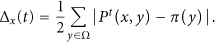
To define mixing time, we must first introduce the relevant notion of distance over time. Let x be the state at time $t=0$ and denote by $P^t(x,·)$ the distribution of the states at time t. The variation distance at time t with respect to the initial state x is defined to be [16]

${\Delta }_x\left(t\right)=\underset{S\subseteq \Omega }{\max }\left|P^t\left(x,S\right)-\pi \left(S\right)\right|.$

(5)

Note that when the state space $\mathrm{\Omega }$ is finite it can be verified that [14]

${\Delta }_x\left(t\right)=\frac{1}{2}{\displaystyle \sum }_{y\in \Omega }\left|P^t\left(x,y\right)-\pi \left(y\right)\right|.$

(6)

Now we may formally define the mixing time as the following function [16]:

${\tau }_x\left(ϵ\right)=\min \left\{t\mid {\Delta }_x\left(t^{\prime }\right)\le ϵ,\mathrm{\hspace{0.17em}\hspace{0.17em}}\forall t\prime \ge t\right\}.$

(7)

A chain 𝔐 is considered rapidly mixing if and only if ${\tau }_x(ϵ)$ is $O(\text{poly}(\log \hspace{0.17em}(n/ϵ)))$ . Clearly, as the name indicates, for a random walk to be used for efficient sampling (according to its stationary distribution), it should be rapidly mixing.

Now, on the way towards proving the rapid mixing property of a random walk, we shall make use of a number of beautiful connections amongst mixing time, the eigenvalues of the Markov chain (in particular the spectral gap, namely, the difference between the first and second eigenvalues), and connectivity properties of the underlying graph as encapsulated by notions called conductance which is a normalized form of expansion. In introducing the connection between expansion and rapid mixing, we note that intuitively graphs with minimal “bottlenecks” have also a lower probability of getting stuck in any particular set of states, and thus a faster mixing time as well. We shall see that the graph-connectivity-based property of “no bottlenecks” is formalized in a continuous manner with the notion of conductance and in a combinatorial manner with expansion. And, then we shall make the relationship between conductance and mixing time precise.

In fact, one of the motivations we have in considering random edge additions to random geometric graphs is precisely based on the nice connectivity properties that random d-regular graphs possess, which we shall see are very much not possessed by random geometric graphs: random d-regular graphs are expanders w.h.p. for $d\ge 3$ . [20, 21]. The combinatorial meaning of this statement is as follows: w.h.p., every subset $S\subset V$ has many edges separating $\text{Cut}(S,\bar{S})$ , particularly $|\text{Cut}(S,\bar{S})|=\alpha d|S|$ for a constant $\alpha >0$ [15]. In general, the expansion of a graph is thus the ratio of the worst case cut divided by the size of the set, and an expander is a graph with constant expansion. Note that the property of a graph being an expander is a much stronger notion than k-connectivity in that it clearly implies an edge connectivity that is at least on the same asymptotic order as the minimum degree, but it further requires that the density of edges separating any set from the rest of the graph is proportional to the size of the set. In fact, being an expander is an extremal property and also much stronger than both the properties of having logarithmic diameter and being rapidly mixing. As such, unsurprisingly, we will not be able to prove that our graphs resulting from random edge additions are expanders. Nonetheless, we will be able to prove sufficient expansion so as to guarantee that the random walk is rapid mixing. We will do so by bounding the conductance.

The conductance of a reversible Markov chain 𝔐 is defined by [17]

$\Phi =\Phi \left(\mathfrak{M}\right)=\underset{S\subset \Omega ,0<\pi \left(S\right)\le 1/2}{\min }\frac{Q\left(S,\overline{S}\right)}{\pi \left(S\right)},$

(8)

where $\bar{S}=\mathrm{\Omega }-S$ , $\pi (S)$ is the probability density of S under the stationary distribution π, and $Q(S,\bar{S})$ is the sum of $Q(v,u)=\pi (v)P(v,u)$ over all $(v,u)\in S\times \bar{S}$ .

In graph-theoretic terms, the conductance of 𝔐 is the minimum over all subsets $S\subset \mathrm{\Omega }$ of the ratio of the weighted flow across the cut $\text{Cut}(S,\bar{S})$ to the weighted capacity of S and as such is clearly a continuous measure of “the degree of no bottlenecks” property. For almost regular graphs of degree $\mathrm{\Theta }(d)$ , we may simplify the expression for conductance as follows:

$\varphi \left(G\right)=\underset{S\subset V}{\min }\frac{\left|\text{Cut}\left(S,\bar{S}\right)\right|}{d\left|S\right|}.$

(9)

And, for this case, it is clear that conductance is a type of normalized measure of expansion where the degree is taken into account as well. Now that we have defined expansion and conductance, we must soon relate these measures to the rapid mixing property. We do this by connecting both conductance and mixing time to the spectral gap.

As the stationary distribution π is defined to be such that $\pi P=\pi$ , it corresponds to the eigenvalue ${\lambda }_0=1$ of P. Let the rest of the eigenvalues of P in decreasing order of absolute value be $1={\lambda }_0\ge |{\lambda }_1|\ge \cdots \ge |{\lambda }_{n-1}|\ge -1$ . For a finite, connected, non-bipartite Markov chain as the one in this work, the rate of convergence to π, which as you may recall is captured by the mixing time, is governed by the difference between the first and second eigenvalues, namely the spectral gap which is $1-{\lambda }_1$ [16]. And, here are the theorems establishing these relationships.

Theorem 9.

For an ergodic Markov chain (ergodicity is guaranteed by the chain being finite, connected, and non-bipartite, as in this work.), the quantity ${\tau }_x(ϵ)$ satisfies

• (i)

${\tau }_x(ϵ)\le {(1-{\lambda }_{\max \hspace{0.17em}})}^{-1}({\ln \hspace{0.17em}\pi (x)}^{-1}+\ln \hspace{0.17em}{ϵ}^{-1})$ ,

(ii)

${\max \hspace{0.17em}}_{x\in \mathrm{\Omega }}{\tau }_x(ϵ)\ge \frac{1}{2}{\lambda }_{\max \hspace{0.17em}}{(1-{\lambda }_{\max \hspace{0.17em}})}^{-1}\ln \hspace{0.17em}{(2ϵ)}^{-1}$ .

And, to relate conductance explicitly to mixing time, it thus suffices to bound the spectral gap with the conductance.

Theorem 10 (see [16]).

The second eigenvalue ${\lambda }_1$ of a reversible Markov chain 𝔐 satisfies

$1-2\Phi \le {\lambda }_1\le 1-\frac{{\Phi }^2}{2}.$

(10)

Combining, as in [14] one has the following.

Corollary 11 (see [17]).

Let 𝔐 be a finite, reversible, ergodic Markov chain with loop probabilities $P(x,x)\ge 1/2$ for all states x. Let $\mathrm{\Phi }$ be the conductance of 𝔐. Then, for any initial state x, the mixing time of 𝔐 satisfies

${\tau }_x\left(ϵ\right)\le 2{\Phi }^{-2}\left({\ln \pi \left(x\right)}^{-1}+\ln {ϵ}^{-1}\right).$

(11)

In particular, the following is immediate too.

Remark 12.

For a random walk to be rapid mixing, it is necessary and sufficient that the conductance be inverse poly-logarithmic.

Finally, we must speak of the mixing properties of the random geometric graph above the connectivity threshold as shown in [14, 18, 19].

Theorem 13.

Given $r=\mathrm{\Omega }(r_{\text{con}})$ , $\varphi (𝒢(n,\mathrm{\Theta }(r)))=\mathrm{\Theta }(r)$ . Similarly, ${\lambda }_2(𝒢(n,r))$ is $\mathrm{\Omega }(r^2)$ and $O(r)$ .

In particular at $\mathrm{\Theta }(r_{\text{con}})$ , ${\lambda }_2(𝒢(n,r))$ is $\mathrm{\Omega }(\log \hspace{0.17em}n/n)$ and $O(\sqrt{(\log \hspace{0.17em}n/n)})$ . This gives a mixing time of $\mathrm{\Omega }(n^{ϵ})$ for $ϵ>0$ . Compare to a rapid mixing Markov chain which requires only $O(\text{poly}\hspace{0.17em}\log \hspace{0.17em}(n))$ steps: possible in wireless network only for very large radius $r=\mathrm{\Theta }(1/\text{poly}\hspace{0.17em}\log \hspace{0.17em}(n))$ , exponentially larger than $r_{\text{con}}$ . Restating, from [14] one has the following

Corollary 14 (mixing time of RGG).

Radius $r=\mathrm{\Omega }(1/\text{poly}(\log \hspace{0.17em}n))$ is w.h.p. necessary and sufficient for $𝒢(n,r)$ to be rapidly mixing.

On the other hand, recall that Even sparse random regular graphs are rapid mixing.

Remark 15.

It is well-known that the random 3-regular graph $G_{R,1}(k)$ is an expander with high probability [20, 22]. Therefore, $G_{R,1}(k)$ also exhibits diameter and average path lengths asymptotically at most logarithmic in its vertex set $|V_R(k)|$ , with high probability.

3. Models of Random Edge Additions

As we start to consider the business of adding random edges to a given initial graph $G_0=(V_0,E_0)$ , note that the set of additional edges $E_R$ and the existing nodes connected by them $V_R\subset V$ form a graph $G_R$ such that the resulting graph $G=(V,E)=G_0+G_R$ has $V=V_0\ge V_R$ and $E=E_0+E_R$ (Such a notation is also consistent with [25].). That is, it is also convenient to view the additional random edges as a new graph $G_R$ superimposed upon the original graph $G_0$ .

Given such a characterization, let us be given a 5-geo-dense geometric graph $G_0=(V_0,E_0)=G(n,r)$ with 5-lattice-skeleton $(L,B_{i,j})$ . In particular, note from Lemma 3 that results apply to any $G_0=𝒢(n,\mathrm{\Omega }(r_{\text{con}}))$ . Given parameter $k\ge 1$ , let vertex set $V_R(k)$ be generated as follows: for any $i,j\le \sqrt{5}/\sqrt{k}r$ , pick a node $v_{i,j}$ uniformly at random from the nodes in the set of bins ${ℬ}_{i,j}={\cup }_{ki\le i^{\prime }\le (k+1)i,kj\le j^{\prime }\le (k+1)j}{B}_{i^{\prime },j^{\prime }}$ (This bin union is simply the formalization of a single contiguous bin $k\times k$ as large as the original bins.), and set $v_{i,j}\in V_R(k)$ . For the case $k=0$ , let $V_R(0)=V_0$ . We now define the various types of random edge sets $E_{R,i}$ for graphs $G_{R,i}(k)=(V_R(k),E_{R,i})$ whose superimpositions upon $G_0$ we shall consider in this work: let $E_{R,1}$ be generated as follows: for every node $v\in V_R(k)$ , pick 3 neighbors in $V_R(k)$ uniformly at random, discarding situations in which any node has degree greater than 3. Thus, the resulting graph $G_{R,1}(k)=(V_R(k),E_{R,1})$ is the random 3-regular Erdos-Renyi graph defined on vertex set $V_R(k)$ . Let $E_{R,2}$ be generated as follows: for every node $v\in V_R(k)$ , pick 1 neighbor in $V_R$ uniformly at random. Thus, the resulting graph $G_{R,2}(k)=(V_R(k),E_{R,2})$ is the random 1-out graph defined on vertex set $V_R(k)$ .

Similarly to the above, let us define the resulting graphs as follows: let $G_1=G_0+G_{R,1}$ . Let $G_2=G_0+G_{R,2}$ Essentially, k controls the frequency of special nodes which shall serve as wired link stations. For $k=\mathrm{\Theta }(1)$ , the frequency is in line exactly with the bins, and thus the occurrence of such wired link stations is 1 in every $\mathrm{\Theta }(n{r}^2)$ . For $r=\mathrm{\Theta }(r_{\text{con}})$ that frequency becomes $\mathrm{\Theta }(1/\log \hspace{0.17em}n)$ , and for larger broadcast radius it is sparser.

Remark 16.

Given $k\ge 1$ , the frequency of wired link stations $|V_R(k)|/|V_0|$ is $\mathrm{\Theta }(1/k^{2}n{r}^2)$ . Namely, the total number of such stations is $|V_R(k)|=\mathrm{\Theta }(1/k^2{r}^2)$ . (Note that clearly k cannot exceed $\mathrm{\Theta }(1/\text{r})$ ).

Before proceeding to prove results on average path lengths for $G_1=G_0+G_{R,i}$ , we note that the manner in which $V_R(k)$ is generated can be simulated approximately by simply choosing a total of logarithmically more wired link stations uniformly at randomly from the original set $V_0$ . This too follows from Coupon Collection.

Remark 17.

For any k, if every $v\in V_0$ is chosen to be a wired link station with probability $\mathrm{\Theta }((\log \hspace{0.17em}(1/k^2{r}^2))/n{k}^2{r}^2)$ , then, with high probability, for every $k^2$ -bin ${ℬ}_{i,j}={\cup }_{ki\le i^{\prime }\le (k+1)i,kj\le j^{\prime }\le (k+1)j}{B}_{i^{\prime },j^{\prime }}$ , there exists a vertex $v^{\prime }\in {ℬ}_{i,j}$ such that $v^{\prime }$ is a wired link station. Moreover, all of the vertices in any $k^2$ bin are almost-equiprobable and almost-independent whp.

Now, we note that the maximum distance of any node in a $k^2$ bin to the corresponding wired link station in the $k^2$ bin is simply bounded by the hop-diameter of the $k^2$ bin.

Remark 18.

Every node is within $\mathrm{\Theta }(k)$ hops of the wired link station in its $k^2$ -bin since the $k^2$ -bin simply stretches the Manhattan distances of the original 5-lattice-skeleton by k.

This remark shall prove relevant in relating inter-node distances in the graph $G=G_0+G_R$ to internode distances in $G_R$ .

As we stated in the introduction, our results regarding mixing time, conductance, and spectral gap will hold for even weaker models of edge addition (or rather link station placement) than those of $G_1$ . However, unlike some of our results for general radius r for diameter and APL, we only lose some generality for conductance results by restricting ourselves to consideration of radius $r=\mathrm{\Theta }(r_{\text{con}})$ in this regime. We present the precise modifications of such models in the section on mixing time bounds.

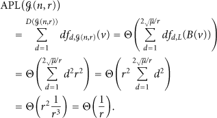
4. APL and Diameter Bounds

4.1. APL and Diameter Bounds for $G_1$

Thus, we now proceed concerning inter-node distances for the first model $G_{R,1}$ .

Combining Remarks 16, 18, and 15, we obtain our first bounds on the resulting average and worst-case path lengths.

Theorem 19.

The diameter and average path lengths for $G_1(k)$ are as follows:

$\begin{array}{cc}\hfill & \text{APL}\left(G_1\left(k\right)\right)\hfill \\ \hfill & \hspace{1em}=O\left(\text{Diam}\left(G_1\left(k\right)\right)\right)=O\left(\min \left\{2k+\log \left(\frac{1}{k^2{r}^2}\right),\frac{1}{r}\right\}\right)\hfill \\ \hfill & \hspace{1em}=O\left(\min \left\{k+\log \left(n\right),\frac{1}{r}\right\}\right).\hfill \end{array}$

(12)

Proof.

Let $s,t\in V$ be arbitrary. s is within k hops to a node $v\in V_R(k)$ and t is within k hops to a node $w\in V_R(k)$ . Moreover, $\mathrm{dist}\hspace{0.17em}(v,w)=O(\log \hspace{0.17em}(|V_R(k)|))$ , making the maximum distance at most $2k+\log \hspace{0.17em}(|V_R(k)|)$ . If r happens to be large, making paths in the original graph (without taking short cuts in $E_{R,1}$ more convenient, then the maximum distance is the diameter of $G_0$ which is $\mathrm{\Theta }(1/r)$ .

For any broadcast radius r, it is clear that when $k=\mathrm{\Theta }(1/r)$ , which is the maximum allowable k and corresponds to the situation of placing a constant number $\mathrm{\Theta }(1)$ wired stations, there is no asymptotic improvement in diameters and average path lengths. However, for any other intermediate k and the lowest reasonable broadcast radius $r=\mathrm{\Theta }(r_{\text{con}})$ , the following may be noted.

Corollary 20.

For $k=O(\log \hspace{0.17em}(n))$ and $G_0=𝒢(n,\mathrm{\Theta }(r_{\text{con}}))$ , $\text{APL}(G_1(k))=O(\text{Diam}(G_1(k)))=O(\log \hspace{0.17em}(n))$ . On the other hand, for intermediate k such that $k=o(n/\log \hspace{0.17em}(n))$ but $k=\omega (\log \hspace{0.17em}(n))$ , one still obtains asymptotic improvement upon the hop lengths in $G_0$ as $\text{APL}(G_1(k))=O(\text{Diam}(G_1(k)))=O(k)=o(\text{Diam}(G_0))$ .

4.2. APL and Diameter Bounds for $G_2$

The case for the second model $G_2$ is not quite as straightforward as that for the first model due to the fact that the random graph $G_{R,2}(k)$ has a positive probability of being disconnected. So, what can we say? It turns out that a lot can be said the moment that $G_{R,2}(k)$ is superimposed directly upon the nodes of any connected graph $G_{\text{init}}$ .

Theorem 21 (expansion of $G_{\text{connected}}+R_{1\text{-out}}$ ; see [25]).

Let $G_0$ be any connected graph. Then $G=G_0+R_{1\text{-out}}$ , which is the graph formed by adding random 1-out edges to every vertex of $G_0$ , is an expander with high probability. In particular, the diameter of G is logarithmic in the vertex set.

Despite the similarities to the situation for $G_1$ , there is the technical issue that the vertex set for $G_{R,2}(k)$ is not identical to the vertex set for $G_0$ but rather asymptotically sparser than such. Therefore, we must understand precisely which graph is an expander, and what that yields for the graph $G_2$ . In particular, we need to extract a connected graph $G_{\text{base}}=(V_{\text{base}},E_{\text{base}})$ that is both a relevant function of the original graph $G_0$ and such that there is a one-to-one meaningful correspondence between the vertex set $V_{\text{base}}$ and $V_R(k)$ to allow application of Theorem 21.

Visually, if we could just contract the lattice subskeleton formed from the $k^2$ -bins into just a $|V_R(k)|$ node lattice, and preserve the meaning of such a contraction for paths in the original graph $G_0$ , then we could apply Theorem 21 to our contraction and then reverse the contraction. We may lose the property of constant expansion upon reversing our contraction for some k, but we will still preserve a bound on path lengths. First, let us state the result, then the proof along the idea above.

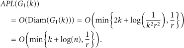
Theorem 22.

The diameter and average path lengths for $G_2(k)$ are as follows:

$\begin{array}{cc}\hfill & \text{APL}\left(G_2\left(k\right)\right)=O\left(\text{Diam}\left(G_2\left(k\right)\right)\right)\hfill \\ \hfill & \hspace{1em}=O\left(\min \left\{k\log \left(\left|V_R\left(k\right)\right|\right),1/r\right\}\right)=O\left(k\log \left(1/r\right)\right).\hfill \end{array}$

(13)

Prior to the theorem proof, let us note the immediate corollary for low broadcast radius, which again notes an exponential improvement in diameter and average path lengths for polylogarithmic k.

Corollary 23.

For $k=\mathrm{\Theta }(1)$ and $G_0=𝒢(n,\mathrm{\Theta }(r_{\text{con}}))$ , $\text{APL}(G_2(k))=O(\text{Diam}(G_2(k)))=O(\log \hspace{0.17em}(n))$ . On the other hand, for intermediate k such that $k=o(n/{\log \hspace{0.17em}}^2(n))$ but $k=\omega (1)$ , one still obtains asymptotic improvement upon the hop lengths in $G_0$ as $\text{APL}(G_2(k))=O(\text{Diam}(G_2(k)))=O(k\log \hspace{0.17em}n)=o(n/\log \hspace{0.17em}(n))=o(\text{Diam}(G_0))$ .

Now let us introduce the theorem proof.

Proof (Proof of Theorem 22).

Consider the graph of node-contractions $G_{\text{contract}}=(V_{\text{contract}},E_{\text{contract}})$ such that each vertex $v_{i,j}\in V_{\text{contract}}$ , is precisely the set of vertices in $k^2$ bin ${ℬ}_{i,j}$ and the edge set $E_{\text{contract}}$ is the two-dimensional lattice appropriately defined on $V_{\text{contract}}$ . We know from Theorem 21 that upon adding random 1-out edges from every $v_{i,j}\in V_{\text{contract}}$ we obtain a graph $G^{\prime }=G_{\text{contract}}+R_{1\text{-out}}$ with diameter logarithmic in $V_{\text{contract}}$ . What does this mean?

Consider any two nodes $s,t\in G_0$ , say that $s\in {ℬ}_{i,j}$ , $t\in {ℬ}_{i^{\prime },j^{\prime }}$ . Let $l=〈v_1,v_2,v_3,\dots ,v_{p-1},v_p〉$ be the shortest path between $v_{i,j}$ and $v_{i^{\prime },j^{\prime }}$ in $G_{\text{contract}}$ (with $v_1=v_{i,j},v_p=v_{i^{\prime },j^{\prime }}$ ). First of all, there is an obvious one-to-one correspondence between the vertex sets $V_{\text{contract}}$ and $V_R(k)$ which does not change the incidence of the random short-cut edges. The only issue occurs when paths in the contracted graph include a lattice edge, and in that case there is a factor $O(k)$ blow-up in the hop number for the original graph. Thus, for any path l in $G_{\text{contract}}$ , we may inductively construct the following path $l^{\prime }$ in $G_{R,2}$ by a sequence of valid subpath replacements in the place of contracted nodes and the edges between them until no contracted nodes and no contracted edges remain (meaning all nodes are actual vertices of our original graph):

• (i)

Base: in accordance with Remark 18, replace $v_1$ in l with the $O(k)$ length shortest path from s to $v_{i,j}$ in $G_0$ . Similarly, replace $v_p$ in l with the $O(k)$ length shortest path from $v_{i^{\prime },j^{\prime }}$ to t in $G_0$ .

(ii)

Inductive case I: for $1<t<p-1$ , let $v_t$ and $v_{t+1}$ be adjacent nodes in the path l that also remain thus far in our path construction. Uniquely define $v_{x,y}\in v_t,v_{x^{\prime },y^{\prime }}\in v_{t+1}$ for $v_{x,y}$ , $v_{x^{\prime },y^{\prime }}\in V_R(k)$ . Either edge $(v_t,v_{t+1})$ is a lattice edge or a random edge. If it is a random edge, then replace $(v_t,v_{t+1})$ of l with the valid wired edge $(v_{x,y},v_{x^{\prime },y^{\prime }})$ . Otherwise, if it is a lattice edge, then there exists a $O(k)$ length shortest path P between $v_{x,y}$ and $v_{x^{\prime },y^{\prime }}$ in $G_0$ from Lemma 7 and Remark 18. Thus, in that case, replace $(v_t,v_{t+1})$ with path P between $v_{x,y}$ and $v_{x^{\prime },y^{\prime }}$ .

(iii)

Inductive case II: let node $v_{x,y}$ be the node following initial wired station $v_{i,j}$ in the construction thus far. Due to the construction, it must be that $v_{i,j}\in v_1$ , $v_{x,y}\in v_2$ . Therefore, similar to inductive case I, either there exists a random wired edge between $v_{i,j}$ and $v_{x,y}$ , or there is a length $O(k)$ path between the two in $G_0$ so replace accordingly. Operate similarly in making the valid replacement for the node $v_{x^{\prime },y^{\prime }}$ preceding final wired station $v_{i^{\prime }{j}^{\prime }}$ .

Clearly, the above construction is valid, replacing contracted edges with valid subpaths at each step. Moreover, at every step, the replacement path is at most a $O(k)$ blow up of a contracted edge. Therefore, the constructed valid path in $G_{R,2}$ is also at most a $O(k)$ multiple of the diameter of $G_{\text{contract}}$ , which we know by Theorem 21 to be logarithmic in $|V_R(k)|$ , which finalizes the proof.

5. Mixing Time and Connectivity Bounds

5.1. Theoretical Bounds on the Mixing Time of $G_1$

Whereas the primary results for this paper concern sparse random edge additions to random geometric graphs, along the way to proving such results, a more general result on the mixing time for sparse random edge additions to arbitrary connected graphs of at most polylogarithmic degree was also found. Further, surprisingly, results on rapid mixing of modifications of random geometric graphs are valid on the weaker model ${\widehat{G}}_1$ in comparison to $G_1$ , thus giving stronger results as well. Let us clarify what we mean by these weaker models before stating formally our results.

To begin with, we only lose some generality for conductance results by restricting ourselves to consideration of radius $r=\mathrm{\Theta }(r_{\text{con}})$ in this regime. Thus, let ${\widehat{G}}_0=𝒢(n,r)$ , where $r=\mathrm{\Theta }(r_{\text{con}})$ such that $r\ge c\sqrt{5/\pi }{r}_{\text{con}}$ for some constant $c>1$ , guaranteeing a 5-geo-dense random geometric graph with high probability. Let k be a given integer parameter. What will differ primarily is not the edge selection mechanism, but rather the node selection mechanism. So, in slight contrast to $V_R(k)$ , let ${\widehat{V}}_R(k)$ be generated as follows: for every node u in $V_0$ , let u belong to ${\widehat{V}}_R(k)$ independently with probability $1/k^2\log \hspace{0.17em}n$ . And, again, for the sake of notation, for $k=0$ , let ${\widehat{V}}_R(0)=V_0$ . The edge selection mechanism is similar to the previous subsection. Let ${\widehat{E}}_{R,1}$ be generated as follows. For every node $v\in {\widehat{V}}_R(k)$ , pick 3 neighbors in ${\widehat{V}}_R(k)$ uniformly at random, discarding situations in which any node has degree greater than 3. Thus, the resulting graph ${\widehat{G}}_{R,1}(k)=({\widehat{V}}_R(k),{\widehat{E}}_{R,1})$ is the random 3-regular Erdos-Renyi graph defined on vertex set ${\widehat{V}}_R(k)$ . For notational convenience, we simply write ${\widehat{G}}_1$ in place of ${\widehat{G}}_{R,1}(k)=({\widehat{V}}_R(k),{\widehat{E}}_{R,2})$ . From Remarks 16 and 17 it is clear that ${\widehat{G}}_1$ is a weaker probabilistic model than $G_1$ , and thus the results concerning them correspond stronger for the most relevant case of $r=\mathrm{\Theta }(r_{\text{con}})$ . In the proof of the results on ${\widehat{G}}_1$ , we will also utilize the following related process: Pick $n^{\prime }=\mathrm{\Theta }(n/k^2\log \hspace{0.17em}n)$ nodes u.a.r from the plane, and these shall constitute ${\widehat{V}}_R(k)$ . It is clear that this node selection process corresponds to the above selection with high probability, as the processes approximate each other as $n\to \infty$ .

Finally, before proceeding to our main results, we present a more general model for $G_1$ , namely, $G_{1}2$ , in the sense that the underlying graph need not be a random geometric one but merely it must be connected and of at most polylogarithmic almostregular degree d and that the edge additions be of any sparse regular expander graph. Let $G_0^{\prime }=(V_0^{\prime },E_0^{\prime })$ be any connected graph such that for $n=|V_0^{\prime }|$ as usual, there exists a function $f(n)=O(\text{poly}\hspace{0.17em}\log \hspace{0.17em}(n))$ for every node $v\in V_{0}2$ the degree $\delta (v)=\mathrm{\Theta }(f(n))$ . Aside from this, as the node set of any graph is identical except for renaming and it is really the edge set that defines a graph, map $V_0^{\prime }$ to ${\widehat{V}}_0$ above, namely, independently at random with identical probability proportional to $1/k^2\log \hspace{0.17em}n$ . And, let the vertex $V_R^{\prime }(k)$ set of the additional random graph be selected from $V_0^{\prime }$ in an identical manner to the selection of ${\widehat{V}}_R(k)$ from ${\widehat{V}}_0$ . Upon this vertex set, we shall superimpose the edges of any given sparse (meaning of constant degree) regular expander $G_{\exp \hspace{0.17em}}=(V_{\exp \hspace{0.17em}},E_{\exp \hspace{0.17em}})$ . So, let $E_{R,1}^{\prime }(k)=E_{\exp \hspace{0.17em}}$ . Note that the edges of $E_{R,1}$ also satisfy the condition of $E_{\exp \hspace{0.17em}}$ by Remark 15. So, it is clear that this model is more general since ${\widehat{G}}_0$ , which is a random geometric graph around the connectivity threshold, clearly satisfies being connected and almost uniform of at most poly-logarithmic degree as required of $G_0^{\prime }$ .

Note that for all variations of $G_1$ (i.e., $G_1$ , ${\widehat{G}}_1$ , and $G_1^{\prime }$ ), the resulting graph is almost regular with high probability, and thus the stationary distribution is almost uniform as well. We now formally state our main theoretical results.

Theorem 24.

The conductance of ${\widehat{G}}_1$ is $\mathrm{\Omega }(1/k^2{\log \hspace{0.17em}}^{2}n)$ with high probability.

From this main theorem this corollary follows immediately from Remark 12.

Corollary 25.

For $k=\mathrm{\Theta }(\text{poly}\hspace{0.17em}\log \hspace{0.17em}(n))$ , ${\widehat{G}}_1$ is rapidly mixing with probability.

In fact, somewhat surprisingly, another more general corollary also follows from the proof of Theorem 24, the consequence of which we shall mention while presenting the main proof shortly.

Corollary 26.

For $k=\mathrm{\Theta }(\text{poly}\hspace{0.17em}\log \hspace{0.17em}(n))$ , $G_1^{\prime }$ is rapidly mixing with probability.

We present the proof of Theorem 24 now and indicate the point to which the arguments apply to Corollary 26 as well.

Proof.

In describing how ${\widehat{V}}_R(k)$ was chosen from amongst $V_0$ , recall that the expected number of selected nodes will be $n/k^2\log \hspace{0.17em}n$ . Let the nodes selected to be in ${\widehat{V}}_R(k)$ be called the red set, and let the remaining nodes constitute the blue set.

From introductory remarks, we may restrict ourselves to this process w.l.o.g.: pick $n^{\prime }=\mathrm{\Theta }(n/k^2\log \hspace{0.17em}n)$ nodes u.a.r from the plane, and make this set the red set. By Theorem 4, any predetermined region of area A such that $nA\ge \log \hspace{0.17em}{n}^{\prime }$ has the same density of red nodes $\mathrm{\Theta }(n^{\prime }A)$ . We can rewrite the condition as follow:

$A\ge \frac{\log n^{\prime }}{n^{\prime }}.$

(14)

The same thing is true for the blue nodes: any predetermined region of area A s.t. $nA\ge \log \hspace{0.17em}n$ has the same density of blue nodes $\mathrm{\Theta }(nA)$ ; this condition means

$A\ge \frac{\log n}{n}.$

(15)

Combining the two conditions, let us first consider areas A that satisfy the following: $A\ge \max \hspace{0.17em}\{\log \hspace{0.17em}n/n,\log \hspace{0.17em}{n}^{\prime }/n^{\prime }\}$ meaning $A\ge \log \hspace{0.17em}n\prime /n\prime \ge \log \hspace{0.17em}n{k}^2\log \hspace{0.17em}n/n\Rightarrow$ meaning

$⟹A\ge \frac{k^2{\log }^{2}n}{n}.$

(16)

We will indicate when we consider what happens for smaller areas.

We note that the above statements are not dependent on the edge set of the underlying graph $G_0$ and thus remain true in the general model too. It should not confuse the reader that the nodes appear to be embedded in the space, as one can always throw any vertex set into the unit square post facto independently.

Now, from Definition  3 consider the conductance measure $\mathrm{\Phi }$ restricted to a given set $X\subset V$ , which we will refer to as ${\mathrm{\Phi }}_X$ , defined as

${\Phi }_X=\frac{\left|\text{Cut}\left(X,V\setminus X\right)\right|}{d\left|S\right|}$

(17)

so that the conductance $\mathrm{\Phi }$ can be naturally defined as follows:

$\Phi =\underset{X\subset V}{\min }{\Phi }_X.$

(18)

Similarly, let $\widehat{X}$ be the set X such that $\mathrm{\Phi }={\mathrm{\Phi }}_{\widehat{X}}$ .

By Coupon Collection Theorem 4 and (16), it follows that if $\widehat{X}\ge k^2{\log \hspace{0.17em}}^{2}n$ , then with high probability $\widehat{X}$ contains $|\widehat{X}{n}^{\prime }/n|\ge k^2{\log \hspace{0.17em}}^{2}n*(n/k^2\log \hspace{0.17em}n)/n\ge \log \hspace{0.17em}n$ red nodes. In general, for such a sufficiently large set $\widehat{X}$ , a frequency $1/k^2\log \hspace{0.17em}n$ of the $\widehat{X}$ nodes is red. Note that we still have not made any use of any geometric property of the edge set except that the combined edge set is almost regular and of at most poly-logarithmic degree. Thus all statements up till now continue to remain true for the general models $G_0^{\prime }$ , $G_1^{\prime }$ , and $G_2^{\prime }$ .

It follows from the construction of $G_1^{\prime }$ that the linked edges expand. In particular, by definition, w.h.p.

$\exists c>0_{\ni }\left|\text{Cut}\left(\widehat{X},V\setminus \widehat{X}\right)\right|\ge \frac{c\left|\widehat{X}\right|}{k^2\log n}.$

(19)

This bound follows from the $E_{\exp \hspace{0.17em}}$ -linked additions alone, and applies to the situation of sufficiently large sets satisfying (16). Thus, the conductance follows from (9) in this case as

${\Phi }_{\widehat{X}}\ge \frac{c}{d_{\text{ave}}{k}^2\log n}$

(20)

with high probability, for average almost uniform degree $d_{\text{ave}}$ .

What happens for small sets $\widehat{X}$ of size less than $k^2{\log \hspace{0.17em}}^{2}n$ ?

Recall that the minimum requirement given for the base graph of the general model $G_1^{\prime }$ was that it be connected and of almost regular polylogarithmic degree $d=\mathrm{\Theta }(\text{poly}\hspace{0.17em}\log \hspace{0.17em}(n))$ . Due to connectivity alone, any cut must have at least one edge. Thus, for such small sets $\widehat{X}$ , we have for both models that

${\Phi }_{\widehat{X}}\ge \frac{1}{d_{\text{ave}}{k}^2{\log }^{2}n}.$

(21)

Substituting polylogarithmic functions for $d_{\text{ave}}$ and k and combining the two cases (20) and (21) yield Corollary 26 for the general case.

For the specific case of the base graph being our relevant model of random geometric graphs about the connectivity threshold, a tighter result can be obtained as small sets exhibit good expansion in such graphs.

For modifications of random geometric graphs in particular, let us guarantee for ${\widehat{G}}_1$ that when $\widehat{X}$ is not sufficiently large, namely, when $\widehat{X}<k^2{\log \hspace{0.17em}}^{2}n$ , that $\widehat{X}$ exhibits sufficient expansion. We show this via the underlying random geometric graph conductance argument itself. In [14], it is noted that in a geo-dense random geometric graph, the worst case conductance for a given set size $|S|$ occurs via the cut with the boundary convex ball, approximated by the convex square, of area A such that $nA=|S|$ . In the situation of small sets, this translates to the square of area A such that $nA<k^2{\log \hspace{0.17em}}^{2}n$ , which gives a side length s such that $s<k\log \hspace{0.17em}n/\sqrt{n}<k\sqrt{\log \hspace{0.17em}n{r}_{\text{con}}}$ . By the same argument for geo-denseness and the lattice skeleton given in the preliminaries as well as in [14], we know that a complete bipartite matching of $\log \hspace{0.17em}n\times \log \hspace{0.17em}n$ edges cuts across every section of length $r_{\text{con}}$ . This means that the size of the cut across side s is approximately $\text{cu}{\text{t}}_s\approx {\log \hspace{0.17em}}^{2}n(s/r_{\text{con}})$ which makes the conductance for such a small set S as follows:

$\begin{array}{c}{\Phi }_S=\Theta \left(\frac{{\log }^{2}ns}{r_{\text{con}}n{s}^2\log n}\right)==\Theta \left(\frac{r_{\text{con}}}{s}\right),\end{array}$

(22)

which by the upper bound on s given above can be lower bounded as follows:

${\Phi }_S\ge \frac{1}{k\sqrt{\log n}}.$

(23)

Returning to the case of large sets $\widehat{X}$ to complete the proof, we need to only substitute $d_{\text{ave}}=\mathrm{\Theta }(\log \hspace{0.17em}n)$ in (20), as the conductance of the larger set will be the dominating factor (in the sense of minimality), obtaining $\mathrm{\Phi }=\mathrm{\Theta }(1/k^2{\log \hspace{0.17em}}^{2}n)$ .

5.2. Experimental Bounds on the Algebraic Connectivity

Experiments were conducted for networks of 100 to 1620 nodes. The networks were constructed in a way that is consistent with the models $G_1$ and $G_2$ of the theoretical section, the parameter k was chosen to be 2, and the radius was chosen to be $r_{\text{con}}$ exactly, with nodes thrown uniformly at random into the unit square and the edge selections generated in accordance with the described random models. Disconnected $𝒢(n,r)$ were discarded from consideration. A caveat in our simulations is that we guaranteed a node in the exact center of each bin, because otherwise there were too many discarded geometric graphs due to lack of connectivity. This problem would not be an issue for sufficiently large networks due to the asymptotic theoretical connectivity guarantee, and anyway comparative results are dominated by how edges are chosen rather than precise node locations.

The results can be seen in Figure 1, where the Y-axis is the spectral gap of the normalized Laplacian, namely, the normalized algebraic connectivity. Notably, the spectral gap for the random geometric graph approaches zero quickly, whereas the spectral gap for $G_1$ and $G_2$ appear to diminish very slowly after 500 nodes. Moreover, note that the number of wired nodes in comparison to the network size n for n values of 100, 300, 800, 1000, 1300, and 1620 are, respectively, as follows: 36, 64, 196, 256, 256, 324. The fraction of wired nodes for the network size of 1620 was just $1/5$ .

Figure 1

Spectral gap comparison for $G_1$ (red), $G_2$ (yellow), and $𝒢(n,r)$ (blue) for network size from 100 to 1620 nodes, radius $r_{\text{con}}$ , and k parameter of 2.

5.3. Observations on Experimental Results

Since we are considering the normalized Laplacian spectral gap, automatically all results must be between 0 and 1. Note that we considered the normalized spectral gap because we want to avoid the scaling problem that could arise if we compared the non-normalized spectra for graphs with very different degrees. Further, we consider the Laplacian instead of simply taking the adjacency matrix, because the Laplacian is symmetric, making faster computations while giving comparable bounds. That all results are less than 0.1 in particular should not be bothersome as well, for two reasons: first, even if we were taking the strong property of being an expander into account, a graph family whose normalized spectral gap never falls below a given constant (e.g., 0.01) would be satisfactory, regardless of the constant. But, we are not attempting to show such a strong property anyway. We are concerned with sufficient expansion, in terms of rapid mixing, which does not even require a constant lower bound, but merely that the rate at which the spectral gap falls is slow (in particular, inverse poly-logarithmic).

In fact, as theoretical result Theorem 24 already demonstrates that $G_1$ is indeed rapid mixing, what is notable in the experimental results is that the (yellow) pattern for $G_2$ is extremely similar to the (red) pattern of $G_1$ . On the other hand, the spectral gap for the underlying random geometric graph $𝒢(n,r)$ , which is theoretically known to have bad expansion [14], falls to zero far more quickly. As we discarded disconnected cases, it is notable that the spectral gap for $𝒢(n,r)$ cannot be zero exactly, although it clearly gets arbitrarily close to zero. What these experimental results reveal in particular is that, similarly to what we have proven above for $G_1$ and also seen now experimentally, $G_2$ also appears to be rapid mixing for k that is not too large.

6. Conclusion

We have presented theoretical bounds on the diameter, APL, conductance, and mixing time of sparse random edge additions onto random wireless networks around the connectivity regime, where our bounds are expressed as functions of the wiring frequency. We have also shown experimental results comparing the normalized algebraic connectivities of the underlying random geometric graph to the hybrid models. In particular, we have shown that when the wiring frequency is at least inverse poly-logarithmic, then the subsequent hybrid network exhibits polylogarithmic diameter and mixing time, both of which are exponential improvements to the wireless network about the connectivity regime. We have also shown that there is correspondingly significant asymptotic improvement to the normalized algebraic connectivity which is known to govern network robustness. Taking broadcast radius on the order of the connectivity threshold is particularly important in the case of sensor networks where energy must be preserved and interference diminished and thus comprises the relevant base graph model as used in much theoretical work on such networks. Nonetheless, the results regarding bounds on diameter and APL are also expressed for general broadcast radii. The mixing time bounds in particular are relevant for distributed gossip applications where it is well established that the performance is dominated by this value. Taken as a whole, this work provides a strong support for hybrid sensor networks.

From a practical standpoint, one may ask how such random wired links should be established atop a wireless sensor network in order that the hybrid model presented be of true relevance. In this regard, we note that the analyses presented is sufficiently general to include an existing sparse wired network atop which a wireless network resides. A benefit of theoretical bounds is precisely this lack of restriction of how the network details are established. In fact, the random edges of the superimposed links need not even be wired, but may be generated via a sufficiently sharply angled and long-ranged directional antenna model as well, as long as the problem of the side lobe may be solved. We point the reader to the existing literature on small worlds for hybrid networks stated in the introduction, as many proposals are given towards the practical aspects of hybrid network creation.

We reiterate that this is the first theoretic graph work to establish solid theoretical foundations of the improvement to graph diameter and mixing time of sparse totally random links (of a nonbroadcast nature) upon a random wireless network above and around the connectivity threshold. The two most relevant works with which to compare and contrast results would be those of [10, 25]. The results of [25] take the base graph to be arbitrary but the wiring probability to so high as to rewire every edge on average. Moreover, that work is concerned with the extremal property of the resulting graph being an expander or not, rather than general expressions of the degree of expansion or mixing time. The arguments used are beautiful and tight, but are neither sufficiently general to take diminishing random wiring probability, nor sufficiently relevant for the base graph being the random wireless domain in particular. The work of [10], in contrast to [25] does consider asymptotically diminishing wiring probability and restricts to the relevant model of wireless base graph around connectivity. However, in that case, base station is fixed and a particular type of greedy forwarding is assumed for the routing protocol, so that they actually obtained the worst results for the case of totally random links. Moreover, they do not discuss the mixing time at all. Thus, our work may be considered to be a positive complementation to that work in the sense that we obtain positive results when routing is both shortest paths-based and random.