A Hole-Tolerant Redundancy Scheme for Wireless Sensor Networks

Abstract

Maximizing network lifetime while not sacrificing coverage and connectivity in wireless sensor networks (WSNs) has attracted many researches during the past few years. One common approach is node scheduling which dynamically schedules some redundant nodes to shut down and keeps alive some necessary nodes to preserve network performance. Previous researches focus either on guaranteeing coverage and connectivity or sacrificing coverage and connectivity to conserve energy. In this paper, we introduce a new hole-tolerant redundancy scheme (HRS) which can prolong network lifetime while maintaining coverage and connectivity performance. This HRS scheme can tolerate some coverage holes when determining redundancy eligibility, so it shuts down more nodes when hole tolerance is higher. Our work takes into account both homoradius WSNs and heteroradius WSNs. The simulation results show that (1) the average coverage percentage varies mildly but network lifetime is prolonged as hole tolerance increases; (2) HRS outperforms several existing lifetime maximization schemes.

1. Introduction

Wireless sensor networks (WSNs) are network systems composed of a large number of inexpensive sensor nodes, deployed in a region to provide monitoring or communication capabilities for commercial or military applications. The positions of sensor nodes need not be engineered or predetermined. This allows random deployment in inaccessible terrains or hazardous environments. Some of the most important application areas of sensor networks include military, natural disasters, health, and the home.

The sensors are unreliable, which have short lifetime, limited power, computational capacities, and memory. They must be regularly recharged or replaced. However, a wild distribution in a complicated environment makes this impossible. To extend the lifetime of a sensor network, one common approach is node scheduling which dynamically schedules sensors between sleep and active cycles based on the cooperative communications and computation among adjacent nodes. It alternately shuts down some redundant nodes and keeps alive some necessary nodes to preserve network performance. Hence, node scheduling in WSNs has become a focus of considerable research in the past few years.

Maximizing the network lifetime while maintaining the degree of coverage and connectivity requested by applications has attracted considerable attention during the past few years [1–4]. However, most of these works have such drawbacks as only focusing on the homogenous sensor network, or having high computing complexity. Thus, trying to solve these problems, our contributions in this paper include three parts.

First, we present a node scheduling scheme that renders the network capable of maintaining monitoring performance with a longer network lifetime. This is a surprising result since prior work either guarantees the degree of coverage and connectivity with more nodes than needed or they sacrifice the degree of coverage and connectivity completeness to save energy. The importance of monitored target area changes with time or site, and it may tolerate some uncovered hole like a part of low monitoring significance. Thus, we take hole tolerance into the consideration which allows more nodes to be shut down when its value is higher.

Second, we introduce a redundancy algorithm applicable when different areas request different degree of coverage. Much research assumes a uniform degree of coverage for the whole area that needs to be monitored. However, some parts of the monitored area are more important than others, for example, in a war scenario, the control center of an enemy army is far more important to be monitored than any other areas. If we maintain the same performance level for all areas, there will be a waste of power in less important monitoring zones. It is essential that the redundancy algorithm be appropriate for different degrees of coverage. Each node sets its requested degree of coverage based on the monitoring priority of the area to which it belongs. Then, the actual degree of coverage is calculated by the redundancy algorithm which decides the redundancy of different nodes separately.

Third, we provide another redundancy algorithm which applies in networks in which sensor nodes have different sensing ranges.

The rest of this paper is organized as follows. After surveying the related work in Section 2, assumptions and preliminaries are presented in Section 3. Section 4 illustrates the proposed node scheduling scheme HRS whose effectiveness is shown by simulation results in Section 5. Finally, we conclude the paper in Section 6.

2. Related Work

We now summarize the typical work that proposes distinctive node scheduling schemes to prolong network lifetime and maintain a good performance.

In [5], the sensor nodes are divided into disjoint sets which are activated successively to perform the area monitoring tasks individually. At any one time, there is only one set active, all nodes in other sets are in a sleep mode. The goal of this approach is to maximize the number of disjoint sets, as this has a direct impact on prolonging the network lifetime. The solution of the problem which is called the SET-K COVER problem is centralized and has been proven to be NP-complete in [6]. In [7], Berman makes an improvement on [5] by not demanding each node belong to only one single set, that is to say some nodes can be in more than one set. Abrams [8] gives another variation of the SET-K COVER problem. It aims to make as many regions as possible to be covered by as many sets as possible, rather than requiring each set to fully cover the monitored area.

In PEAS [9], each node broadcasts a probe message after sleeping for a random period and enters the on-duty mode only if it receives no replies from neighbors within transmission range; otherwise, it will stay in the sleep mode. Though this method is decentralized, offering high scalability and low cost, it cannot guarantee the degree of coverage. When a node goes to sleep, it may cause a coverage hole.

Paper [10] proposes a distributed scheduling mechanism which, called TIAN hereinafter, can preserve sensing coverage. The mechanism allows a sensor to turn off only if its sensing area is completely covered by its neighbors' sensing areas. The neighbors are called this node's off-duty sponsors, and the sector that a neighbor covers with its sensing area is called a sponsored sector. However, this mechanism only considers those neighbors located within a node's sensing area to be potential off-duty sponsors, while other neighbors are ignored even if their coverage may overlap with this node's sensing area, so this solution may underestimate the number of sensors that can be turned off. Besides, it only guarantees 1-degree coverage which reduces scalability.

Some work is done to give a sufficient and necessary condition to find out off-duty eligible nodes. Huang et al. [11] and Liu et al. [12] propose perimeter coverage algorithms, by which they calculate the coverage degree of every arc on a node's sensing circle to judge if the node is redundant or not. The conditions proposed in these algorithms are sufficient and necessary, but the computing complexity is too high. Paper [13] proposes a protocol called CCP which is able to configure itself to any feasible degree of coverage and connectivity in order to support different applications and environments with diverse requirements. This flexibility allows the network to self-configure for a wide range of applications and environments. But this mechanism has a quite high computing complexity of $O(n^3)$ , where n denotes the number of neighbors of the sensor. Paper [14] extended to arbitrary region. Zhang and Hou [15] propose a distributed mechanism, optimal geographic density control (OGDC), to maximize the number of sleeping sensors while ensuring that the working sensors provide complete 1 coverage and 1 connectivity. OGDC tries to minimize the overlapping area between the working sensors. OGDC's protocol is quite similar to that of the sponsored sector mechanism, except that they use different on-duty/off-duty eligibility rules and the sponsored sector mechanism is more conservative when turning off sensors.

To sum up, existing work on node scheduling has the following characteristics. (1) They cannot achieve a good balance between prolonging the network lifetime and guaranteeing the degree of coverage and connectivity with low computing complexity. (2) Much research assumes a uniform coverage degree for the area that needs to be monitored. (3) They focus on WSN whose nodes have the same sensing and transmission radius (we call it homoradius WSNs). We will try to solve these problems in this paper.

3. Network Model and Preliminary

3.1. Network Model

We consider a WSN consisting of a set S of n static sensor nodes. Each node $u\in S$ can sense events of interest in its sensing range and communicate with nodes in its transmission range. We make the natural assumption that there are no two sensors at the same location. The sensors are distributed over the monitoring area, a large 2-dimensional area that we are interested in monitoring. The monitoring area is typically significantly larger than the sensing range of a single sensor.

For any sensor node u whose sensing radius and communication radius are $\text{Rs}(u)$ and $\text{Rc}(u)$ , its sensing area $S(u)$ and transmission area $T(u)$ are open discs, centered at u, with radius $\text{Rs}(u)$ and radius $\text{Rc}(u)$ , respectively, and we assume $\text{Rc}(u)>2\text{Rs}(u)$ under which condition, network coverage implies network connectivity. Each point in $S(u)$ is said to be covered by node u. Any two sensor nodes u and v are termed adjacent or neighbors if they are located within the transmission area of each other. If a point in monitored area is covered by and only by k different nodes (neighbors), we call this point is k-covered, and the coverage degree of this point is k. For any area, if it requests all the points in this area having a coverage degree no less than k, we call this area has a requested coverage degree of k. For any node u, if its sensing range can guarantee its requested coverage degree by its neighbors, u is a redundant node and can be turned off.

3.2. Preliminary and Problem Statement

In this paper, we focus on the hole-tolerant scheme in both homoradius and heteroradius WSNs. A WSN is a homoradius WSN if all its sensors have the same sensing and transmission radius. Otherwise, it is a heteroradius WSN.

In hole-tolerant scheme, the WSN can tolerate coverage hole(s) in the monitor area to some extent. For a monitor area with a requested coverage degree of k, one of its subarea is called a coverage hole if this subarea is less than k-covered. The percentage of the subarea whose coverage degree is at least k to the whole monitor area is called coverage percentage. In hole-tolerant WSN, the network can fulfill normal monitor when the coverage percentage is no less than a specific value. We define a parameter hole tolerance which indicates the biggest coverage hole a WSN can withstand before normal monitoring operation is impaired.

Before we state the problem, let us give two necessary definitions, namely, contributing node and contribution angle. Suppose nodes u and v are neighbors in Figure 1, v is a contributing node (to node u) if v's coverage to $S(u)$ is taken into consideration in the redundancy decision phase (shown in Section 4.2). Suppose both sensing areas $S(u)$ and $S(v)$ intersect at points $P_1$ and $P_2$ , then angle α is defined as the contribution angle of node v to node u, $L_{uv}$ and $R_{uv}$ are the left bound and right bound of this contribution angle between node u and v.

Figure 1

Contributing angle.

With the definition above, the problem this paper tries to solve lies in the following. (1) Similar to TIAN, how to provide a redundancy decision scheme by explore the relationship among contributing angles of different neighbors. (2) How can this scheme achieve high performance without underestimation or overestimation as well as possible? (3) How can this scheme provide configuration of different requested coverage degree and can be used in hole-tolerant WSNs?

4. Lifetime-Extending Scheme HRS

Our scheme consists of three parts: initialization, redundancy decision, and status transfer. The initialization phase randomly distributes the sensors, informing each sensor of some parameters. In the redundancy decision phase, each sensor node runs the redundancy algorithm to decide its eligibility to turn off. If it is eligible, then the node shifts to the status transfer phase which puts the node into a sleep mode properly. The following sections will describe them in detail.

4.1. Initialization

An initialization phase is executed at the beginning of the network operation. During the initialization phase, each sensor acquires the following local information: location, sensing range, initial status, remaining energy, and requested coverage degree.

If the whole monitoring area in our network model is composed of subareas with different requested coverage degree, how can we set the requested coverage degree for a sensor u when judging its off-duty eligibility. If the sensing area of u is within one subarea, u's requested coverage degree is equal to the requested coverage degree of this subarea. If the sensing area of u is divided by more than one subareas, we use the demanded coverage degree of the sub-area which is the nearest to a sensor u as u's requested coverage degree when judging its off-duty eligibility.

4.2. Redundancy Decision

4.2.1. Redundancy Decision in Homoradius WSN

In the redundancy decision phase, a sensor node runs the redundancy algorithm to figure out if it is eligible to go to the sleep mode. Algorithm 1 provides the redundancy decision algorithm in homoradius WSN.

Algorithm 1: The redundancy algorithm in homoradius WSN.

Begin

Input Kr(n), Rs(n), toler

   /* Kr(n) are the demanded coverage degrees for all nodes

   /* Rs(n) are the sensing radius for all nodes

   /* toler is hole tolerance of the WSN.

(1) $D_1$ = 0

(2) $D_2$ = $\text{Rs}(u)$

(3) while $D_2\le (1+\sqrt{\text{toler}})\text{Rs}(u)$ do

(4)   for each node v of u's neighbors

(5)   if $D_1<d(u,v)\le D_2$   then

(6)    calculate the left bound ${\alpha }_L$ (u,v) and right bound ${\alpha }_R$ (u,v) of the contribution angle

(7)   end if

(8)   end for

(9)   calculate the coverage degree of each bound point to get the minimum coverage degree $K_{\min \hspace{0.17em}}(u)$

(10) if $K_{\min \hspace{0.17em}}(u)\ge \text{Kr}(u)$  then

(11)   Return eligible =1/* node u is eligible to be turned off

(12) else

(13)    $D_1$ = $D_2$

(14)    $D_2$ = $D_1$ + Δd/*Δd is the step size

(15) end if

(16) end while

(17) Return eligible = 0/* node u is not eligible to be turned off

End

Consider two sensors u and v located in $(x_u,y_u)$ and $(x_v,y_v)$ , respectively. Denote the distance between u and v by $d(u,v)=\sqrt{{|x_u-x_v|}^2+{|y_u-y_v|}^2}$ .

As shown in Figure 1, we take the contribution angle α as an approximation of the sector (denoted by $S_{u,P_1\to P_2}$ ) bounded by radius $u{P}_1$ , radius $u{P}_2$ , and inner arc $P_1{P}_2$ . That is to say, we assume the sensing area of node v with a contribution angle α (to sensor node u) covers $S_{u,P_1\to P_2}$ . Though there is a coverage hole in $S(u)$ , with the tolerance parameter toler, we know that this assumption will not affect monitoring operation too much, which can be seen from the simulation results in Section 5.

We gradually increase the contributing nodes loop by loop as illustrated in Figure 2 (by step 14 in Algorithm 1). Initially, the contributing nodes are within area 1, then, we add nodes in loop area 2 as contributing nodes, next, loop area 3, and so on. Obviously, there will be an increase in coverage holes as contributing nodes are added, and this is where the flexibility of our intelligent algorithm comes into its own.

Figure 2

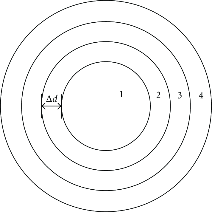
Increase of contributing nodes.

The algorithm operates as follows: we define a contributing node v as one whose distance to u is within $(D_1,D_2$ ], where $D_1=0$ , $D_2=\text{Rs}(u)$ for initialization.

Step 1.

For each contributing node v, we determine the left bound $L_{uv}$ and right bound $R_{uv}$ of the contribution angle.

Step 2.

Place all the points $L_{uv}$ and $R_{uv}$ on the line segment $[\mathrm{0,2}\pi ]$ which is considered end-to-end, and mark them with node $id$ and the flag L or R.

Step 3.

Determine the coverage degree of each point gotten in Step 2. In Figure 3, a coverage degree of a point, P, demonstrates the coverage degree of the angle range bounded by P and its nearest left neighbor on the segment. For example, coverage degree of point $L_{u3}$ demonstrates the coverage degree of the angle $[R_{u7},L_{u3}]$ . Operation is as follows.

For each point on the line segment $[\mathrm{0,2}\pi ]$ , if it is marked as “R”, then visit points from right to left starting from its first left neighbor until meeting the point with the same node $id$ as itself, increase the coverage degree of all the nodes covered during the traverse, respectively, by 1 degree.

If the minimum coverage degree of all the angle ranges is not smaller than the demanded coverage degree of $S(u)$ , then u is redundant, end the process. Else, go to Step 4.

Figure 3

Line segment coverage diagram.

Step 4.

Let $D_1=D_2$ , $D_2=D_2+\mathrm{\Delta }d$ ( $\mathrm{\Delta }d$ is a small step size to increase the range), if $D_2\le (1+\sqrt{\text{toler}})\text{Rs}(u)$ ; then, add neighbors whose distance to u is within $(D_1,D_2]$ into contributing nodes, and go to Step 1; else, end the process.

We now explain more about the parameters in the algorithm. First, we can set $D_1=0$ , $D_2=\mathrm{\hspace{0.17em}\hspace{0.17em}}(1+\sqrt{\text{toler}})\text{Rs}(u)$ directly as we do in heteroradius WSN in Section 4.2.2, then all nodes whose distance to u are within $(0,(1+\sqrt{\text{toler}})\text{Rs}(u)]$ are taken into computation of the coverage degree. The reason why we bother to increase the contributing nodes loop by loop is that, when the nodes are densely scattered, the algorithm can finish the computation earlier to get a higher efficiency.

Second, the value of $\mathrm{\Delta }d$ influences the performance of the algorithm, for example, convergence rate. We can adjust it according to the nodes density, whether there exists a best value for each density needs a further study.

With the hole tolerance parameter, toler, we achieve a tradeoff between network performance and lifetime. From the condition: $d(u,v)\le (1+\sqrt{\text{toler}})\text{Rs}(u)$ , we can see that the larger toler is, the more contributing nodes are used and a greater number of coverage holes occur which also means poorer network performance. However, at the same time, more nodes will be determined to be redundant, so we will achieve a longer network lifetime.

Let us explain the condition $d(u,v)\le (1+\sqrt{\text{toler}})\text{Rs}(u)$ .

In Figure 4, we see node v is a distant contributing node of node u, both have a sensing range of $\text{Rs}(u)$ . The circle centered at u with radius $(d(u,\mathrm{\hspace{0.17em}\hspace{0.17em}}v)-\text{Rs}(u))$ is a definite coverage hole. Without lose of generality, we assume the area of coverage holes in other areas of $S(u)$ is ε ( $\epsilon \ge 0$ ), then

$\frac{\pi {\left(d\left(u,v\right)-\text{Rs}\left(u\right)\right)}^2+\epsilon }{\pi \text{Rs}{\left(u\right)}^2}=\text{toler}.$

(1)

Figure 4

Condition explanation.

So we get $d(u,\mathrm{\hspace{0.17em}\hspace{0.17em}}v)\le (1+\sqrt{\text{toler}})\text{Rs}(u)$ .

Now, we will show how the algorithm works by an example. Suppose node u has 8 neighbors as shown in Figure 5(a), and the demanded coverage degree is 1.

Figure 5

Example of the algorithm.

First, for each contributing node directly within our sensing range, 1, 3, 5, and 7, calculate the left and right bounds, and mark them with node $id$ and flag L or R as in Figure 5(b).

Second, mark the covered areas on a line segment coverage diagram as shown in Figure 3.

Third, calculate the coverage degree of each point. In Figure 6, we visualize the coverage for each section of the line segment coverage diagram. We can see that the minimum coverage degree is 1, which is the demanded coverage degree, so node u is determined to be redundant. If the required coverage degree is 2, we would have to add more neighbors as contributing nodes by increasing the radius of our comparison loop.

Figure 6

Line segment with coverage degree.

4.2.2. Redundancy Decision in Heteroradius WSN

In heteroradius WSN, the redundancy algorithm is provided in Algorithm 2 and shares most of the characteristics of the homoradius WSN, so next we only describe the different parts.

Algorithm 2: The Redundancy Algorithm in heteroradius WSN.

Begin

Input $\text{Kr}(n)$ , $\text{Rs}(n)$ , toler

   /* $\text{Kr}(n)$ are the demanded coverage degrees for all n nodes

   /* $\text{Rs}(n)$ are the sensing radius for all n nodes

   /* toler is hole tolerance of the WSN.

(1) for each node v of u's neighbors

(2) if   $\text{Rs}(u)>\text{Rs}(v)$ && $d(u,v)<\text{Rs}(u)-\text{Rs}(v)$  then

(3) continue

(4) end if

(5) if $\text{Rs}(u)<\text{Rs}(v)$ && $d(u,v)<\text{Rs}(u)-\text{Rs}(v)$  then

(6) add 1 coverage degree to each existing bound point

(7) else

(8) if $d(u,v)\le \text{Rs}(v)+\sqrt{\text{toler}}\text{Rs}(u)$  then

(9) Calculate the left bound ${\alpha }_L$ (u,v) and right bound ${\alpha }_R$ (u,v) of the contribution angle

(10) end if

(11) end for

(12) Calculate the coverage degree of each bound point to get the minimum coverage degree $K_{\min \hspace{0.17em}}(u)$

(13) if $K_{\min \hspace{0.17em}}(u)\ge \text{Kr}(u)$  then

(14) Return eligible = 1/* node u is eligible to be turned off

(15) else

(16) Return eligible = 0/* node u is not eligible to be turned off

End

Suppose the sensing radius of node u and v meets $\text{Rs}(u)<\text{Rs}(v)$ , their relative position is shown in Figure 7. Though $0<d(u,v)\le \text{Rs}(u)$ , we cannot calculate the left and right bounds of the contribution angle, $L_{uv}$ and $R_{uv}$ , since there is no such angle. In this case, we add 1 coverage degree to each existing coverage line segment.

Figure 7

A different case between heteroradius WSN and homoradius WSN.

4.3. Status Transfer

Each node determines its redundancy using the redundancy algorithms (See Algorithms 1 and 2) and may switch status dynamically when its redundancy eligibility changes. Redundant nodes should enter sleep mode, while nonredundant ones are working. However, if more than one node goes to sleep simultaneously, it may cause coverage hole; or if they turn active at the same time, network energy may be wasted. To resolve this problem, different collision prevention mechanisms or scheduling schemes are introduced into this field [10, 11]. But this is still an open issue. Thus, in this paper, we also introduce a different mechanism. But the main contribution of this paper is that it proposed algorithms for nodes to acquire their off-duty eligibility (i.e., to determine if they are redundant or not). Also, our algorithms are independent to the collision prevention mechanisms. So, in the analysis and simulation part, we only focus on evaluating the performance of Algorithms 1 and 2. Evaluating and further research on the collision prevention mechanism are our future work.

Now, we describe in detail this mechanism. Each sensor at any moment is in one of the following five states: ACTIVE, that is, the sensor monitors its monitoring region and communicates with other sensors; SLEEP, that is, the node is put into a low power mode to save energy; JUDGE: the sensor collects information of its neighbors and runs the redundancy decision algorithm; OFF-DELAY: the sensor waits for a period before going to SLEEP; ON-DELAY: the sensor waits for a period before going to ACTIVE.

• (1)

When a node is in ACTIVE state: we trigger a timer $T_a$ , if the sensor is going to run out of energy, it sends a Drop message and then goes to SLEEP, else, if $T_a$ expires, it switches to the OFF-DELAY state.

(2)

When nodes being in SLEEP state: when a sensor goes sleep, we start a timer $T_{\text{sp}}$ which makes each sleep node wake up after a certain period of time. When it expires, the sensor transfers its state to the JUDGE state.

(3)

When nodes being in JUDGE state: in this state, the sensor does two things. First, it broadcasts a Hello message to regenerate its neighbor table and learn their positions from its neighbors' reply messages. Then, it runs the redundancy decision algorithm to determine whether it is redundant or not. It transfers to the ON-DELAY state if it is not redundant; else it enters the OFF-DELAY state.

(4)

When nodes being in ON-DELAY state: we set a timer $T_{\text{ond}}$ , if the sensor receives a Join message, then it goes back to the JUDGE state. If $T_{\text{ond}}$ expires, the sensor switches to ACTIVE and sends a Join message.

(5)

When nodes being in OFF-DELAY state: set a timer $T_{\text{offd}}$ . If the sensor receives a Drop message, then it goes back to the JUDGE state. If $T_{\text{offd}}$ expires, the sensor sends a Drop message and goes to SLEEP.

The values of the timers will affect the responsiveness of HRS. $T_a$ and $T_{\text{sp}}$ should be considerably greater than $T_{\text{ond}}$ and $T_{\text{offd}}$ , otherwise nodes may spend too much time in decision states and thus no long enough time for sleep. But they must not be too much greater, otherwise the decisions cannot be made timely, and thus there may be many coverage holes appear or additional unnecessary redundancy may occur. Moreover, these timers are related to the remaining energy. For example, a node with more remaining energy should increase $T_a$ to balance energy consumption of the network. In addition, the density of nodes in the network has an effect on the timers. For example, for a denser network where a node has more neighbors, $T_{\text{ond}}$ and $T_{\text{offd}}$ should be long enough for a node to collect all the Join or Drop messages from its neighbors. Whether there exist any optimal values for these timers is left as our future work.

Figure 8 provides a useful visualization of the status transfer in an FSM.

Figure 8

Status transfer FSM.

5. Analysis and Simulation

Now, we evaluate the performance of HRS by simulations. Similar with CCP and TIAN, we also let each node decide whether to turn off or not in a random sequence, and the decision of each node is visible to all the other nodes. Namely, according to this random sequence, after calculating its actual coverage degree by HRS, CCP, or TIAN, each node compares this degree with the requested coverage degree. If the former is no less than the later, this node turns itself off.

We have taken monitored area as $20\hspace{0.17em}\times \hspace{0.17em}20$ units, demanded coverage of 1. We experimented with 50 to 600 sensor nodes, with sensing and transmission ranges of 2 and 5 units, respectively. All sensor nodes are positioned according to uniform random distribution. We uniformly assigned initial energy of 300 units to each sensor node. According to the research about the energy consumption in paper [16], we assume that the energy each node consumes for redundancy decision (including in the temporary status as ON-DELAY and JUDGE), SLEEP and ACTIVE are 0.5, 1, and 10, respectively. In our simulations, the toler for each node set ranges from 0 to 0.8, increasing by 0.1 each time. We do two sets of simulations. The first one tests the impact of hole tolerance on network coverage and lifetime, and the second one evaluates the performance of HRS. In all of our simulations, we assume the sensing network is alive until the network coverage percentage is less than 50% (including the simulation of CCP and TIAN in this paper).

5.1. The Impact of Hole Tolerance

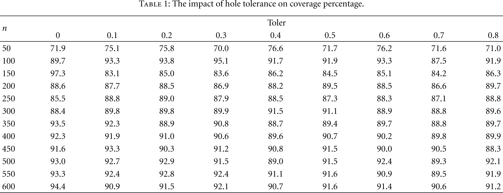
All nodes run HRS independently. We compute the network coverage percentage at every time slot until the coverage percentage of the network is lower than a demanded limit (we set it as 50% here) and then figure out the average coverage percentage. The results are shown in Table 1 and Figure 9. We can see that, for a certain number of nodes, the average coverage percentage does not appear to be much affected by the hole tolerance level.

Table 1

The impact of hole tolerance on coverage percentage.

n	Toler
	0	0.1	0.2	0.3	0.4	0.5	0.6	0.7	0.8
50	71.9	75.1	75.8	70.0	76.6	71.7	76.2	71.6	71.0
100	89.7	93.3	93.8	95.1	91.7	91.9	93.3	87.5	91.9
150	97.3	83.1	85.0	83.6	86.2	84.5	85.1	84.2	86.3
200	88.6	87.7	88.5	86.9	88.2	89.5	88.5	86.6	89.7
250	85.5	88.8	89.0	87.9	88.5	87.3	88.3	87.1	88.8
300	88.4	89.8	89.8	89.9	91.5	91.1	88.9	88.8	89.6
350	93.5	92.3	88.9	90.8	88.7	89.4	89.7	88.8	89.7
400	92.3	91.9	91.0	90.6	89.6	90.7	90.2	89.8	89.9
450	91.6	93.3	90.3	91.2	90.8	91.5	90.0	90.5	88.3
500	93.0	92.7	92.9	91.5	89.0	91.5	92.4	89.3	92.1
550	93.3	92.4	92.8	92.4	91.1	91.6	90.9	89.5	91.9
600	94.4	90.9	91.5	92.1	90.7	91.6	91.4	90.6	91.2

Figure 9

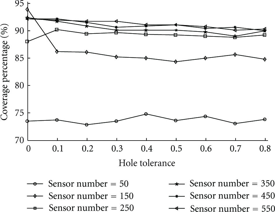
Coverage percentage affected by hole tolerance.

Next, we examine how hole tolerance affects network lifetime. Figure 10 shows a 3D surface plot of the network lifetime for different hole tolerance values. We can see that increasing the hole tolerance of the network results in a longer network lifetime. To have a clearer view, we calculate the average lifetime of WSNs with different number of nodes (say 200, 400, or 600 in our simulations) and different hole tolerance (say from 0.1 to 0.8 in our simulations). As shown in Figure 11, it is clear that the increase in hole tolerance from 0 to 0.4 has a great effect after which its performance increase is much less. We can also get the information that gives a certain network (obviously the node number is certain), then network lifetime will be increased as tolerance increases.

Figure 10

The impact of hole tolerance.

Figure 11

Hole tolerance versus network lifetime.

From Figure 11, we can easily observe that the curves representing the results gotten from WSNs with more nodes are steeper than those gotten from WSNs with fewer nodes. This is because of the little coincidence phenomena. That is to say, when the number of nodes is small, the nodes are sparsely scattered so that there is little or no coincidence of any two sensing area. In this case, the increase of toler has little effect on the network lifetime. Thus, our HRS scheme fits denser network better. Since WSN is normally composed of a large number of sensor nodes by definition, our scheme fits WSN very well.

From the above two experiments, we see that average coverage percentage varies moderately and the hole tolerance does not have obvious effect on it. However, network lifetime is increased to a certain degree by increasing hole tolerance, though, after 0.4, the increase is much less. So we can achieve a longer network lifetime when using our hole tolerance mechanism.

5.2. The Performance of HRS

This experiment compares the performance of our HRS to two very popular protocols TIAN and CCP. Similar to HRS, TIAN and CCP are decentralized protocols designed to preserve coverage by turning off redundant nodes to conserve energy in a sensor network. The eligibility rules in the TIAN protocol, CCP, and HRS are different. The main advantage of HRS lies in its ability to configure the network to a specific hole tolerance level, which is not supported in TIAN and CCP protocols.

We perform the same experiment as before with HRS using tolerance levels of 0, 0.4, and 0.8. The experiment results, displayed in Figure 12, show that, even when hole tolerance is 0.8 (toler = 0.8), HRS gets close to the same average coverage percentage as TIAN and CCP. When toler = 0, the curve of HRS and TIAN almost coincide, which means, through the tolerance modulation, HRS can achieve the same coverage performance as TIAN. We then compare the average number of alive nodes gotten by different schemes. As can be seen from Figure 13, when the hole tolerance is greater than 0 (toler > 0), HRS has a considerably smaller number of active nodes and hence leads to more energy conservation than the other two protocols do. We subsequently draw a picture of the lifetime comparison in Figure 14 from which we clearly see that HRS gets longer lifetime than others as we expect.

Figure 12

Average coverage percentage comparison.

Figure 13

Average alive node number comparison.

Figure 14

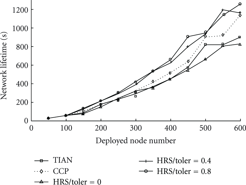
Network lifetime comparison.

5.3. Complexity Analysis

Now, we analyze the communication complexity and computing complexity of these three algorithms. For the communication complexity, since HRS, CCP and TIAN all need and only need to collect neighbor nodes to determine the off-duty eligibility by communication, their communication complexity is similar.

For the computing complexity, as can be seen from the steps HRS follows, the step to calculate the coverage degree of each bound point to get the minimum coverage degree takes the longest time. This step has a computing complexity of $O(n\log \hspace{0.17em}n)$ to sort all the left and right bounds of contribution angles by Quicksort, while all the other steps with the computing complexity of or less than $O(n)$ . Thus, the total computing complexity of HRS is $O(n\log \hspace{0.17em}n)$ , which is much lower than CCP of $O(n^3)$ . Since our work focuses on the redundant WSNs where the number of nodes is large and each node may have enough neighbors, this decrease is significant in entire networks. The computing complexity of TIAN is similar to that of HRS, while HRS performs better than TIAN.

6. Conclusion and Future Work

In this paper, we have designed a hole-tolerant redundancy scheme, HRS, for WSNs. This scheme introduces a parameter, called hole tolerance, which renders the network capable of varying from 100% strict coverage performance to moderately poorer ones to achieve longer network lifetime. It allows different areas to set different requested coverage degrees, and it is applicable in both homoradius networks and heteroradius networks.

Our experiments show that hole tolerance has no remarkable impact on average coverage percentage and that network lifetime will be extended as hole tolerance is increased. We also compare the performance of HRS with another two famous schemes, TIAN and CCP. HRS achieves a similar average coverage percentage to TIAN and CCP, and using hole tolerance can reduce the number of active nodes resulting in a considerable increase in network lifetime.

For future work, on the one hand, we will evaluate and do more research on the collision prevention mechanism proposed in this paper. On the other hand, HRS is a hole-tolerant scheme, the network can fulfill normal monitor task when the coverage percentage is not less than a specific value. We demonstrated how the hole tolerance affects the coverage percentage. But we did not give the mathematical relationship between hole tolerance and coverage percentage. This would be our future work.