Sage Journals: Discover world-class research

Abstract

Neighbor discovery is a component of communication and access protocols for ad hoc networks. Wireless sensor networks often must operate under a more severe low-power regimen than do traditional ad hoc networks, notably by turning off radio for extended periods. Turning off a radio is problematic for neighbor discovery, and a balance is needed between adequate open communication for discovery and silence to conserve power. This paper surveys recent progress on the problems of neighbor discovery for wireless sensor networks. The basic ideas behind these protocols are explained, which include deterministic schedules of waking and sleeping, randomized schedules, and combinatorial methods to ensure discovery.

1. Introduction

In the decade following the introduction of Wireless Sensor Networks (WSNs) to the lexicon, the technical landscape of applications, network protocols, and research problems has shifted somewhat. The early focus on basic communication issues enabled more applications to be deployed, and the catalog of available WSN platforms increased to include many types of radio and processor features. Experience with applications and platforms showed that early perceptions of power challenges and solutions to power management were perhaps misinformed. For example, the lifetime of a sensor node running on battery was not significantly extended by attenuating transmission power. Rather, the most effective means of power conservation consists in powering off components entirely, including sensors and the radio. The appendix of this paper has a small example illustrating how the lifetime of a battery-powered sensor node could vary from days to years depending on effective use of sleep modes. Scheduling operations across a WSN, for example, selectively powering on and off nodes, is a problem of distributed control. Indeed, a fundamental balance is needed to minimize power utilization on one hand, yet facilitate application data forwarding through the WSN on the other hand. The situation is yet more challenging if the network topology is dynamic, nodes are mobile, or nodes depend on harvesting devices to scavenge sufficient power for radio operation.

This paper surveys the literature of one facet of power management in sensor network protocols, namely the problem of neighbor discovery. Informally, the problem is to devise an efficient protocol whereby sensor nodes learn of the presence of other nodes within communication range even as they adhere to low-power operation, with the radio mostly off. The crux of the problem is as follows.

A sensor node p needs to communicate with some neighbor q, but that is only possible when both p and q have their radios powered on at the same time.

This problem is particularly relevant to ad hoc or mobile deployments where the set of (communication) neighbors of a node is unpredictable or dynamic. The parameters of the problem are many: design choices for power schedules, constraints of processor (resources and timing facilities), hardware features of the radio, and application requirements control what is the set of conceivable solutions. Though several techniques from the literature on neighbor discovery have some combinatorial flavor, the dependence on problem parameters makes framing neighbor discovery as a purely algorithmic problem somewhat difficult. To give the survey context, we examine some related problems, technology and older results from areas of networks and distributed computing. The survey then explains prominent techniques for neighbor discovery, metrics for analysis, and several important results from the literature. We have also simulated representative protocols for neighbor discovery, to illustrate for the reader how different design choices affect performance metrics.

Organization. For readers unfamiliar with the problem of neighbor discovery, Section 2 discusses a brief motivating scenario. The paper then presents historical background, sensor node and radio platform considerations before presenting protocols in Section 5 (eager readers may wish to start with Section 5). After reviewing some background concepts from distributed computing in Section 3, considerations that constrain and affect evaluation of protocols are discussed in Section 4. Material in Section 5 organizes neighbor discovery protocols thematically, grouping them by their basic discovery techniques (which mostly repeat historical themes mentioned in Section 3). Section 6 is devoted to performance metrics for neighbor discovery protocols. Final remarks are in Section 7. Some details about hardware and protocols considerations are deferred to the appendix.

2. Motivating Scenario

Protocols for low-power operation in sensor networks turn the radio off between communications. Schedules for turning radio on and off could be periodic, random, or some hybrid of these approaches. Figure 1 shows a scenario for four nodes, (1)–(4). The top part of the figure shows the communication network, which is a linear structure (node (1) is out of range of node (3)). Each of these nodes uses the same periodic awake schedule, waking once every five time intervals. Unfortunately, their schedules are not coordinated in the figure; hence no two nodes are unable to communicate, because their radios are not on at the same time. This unfortunate situation could be the result of improper initialization, crash and restart events at unpredicted times, or the normal dynamic arrival of nodes in an ad hoc WSN.

Figure 1

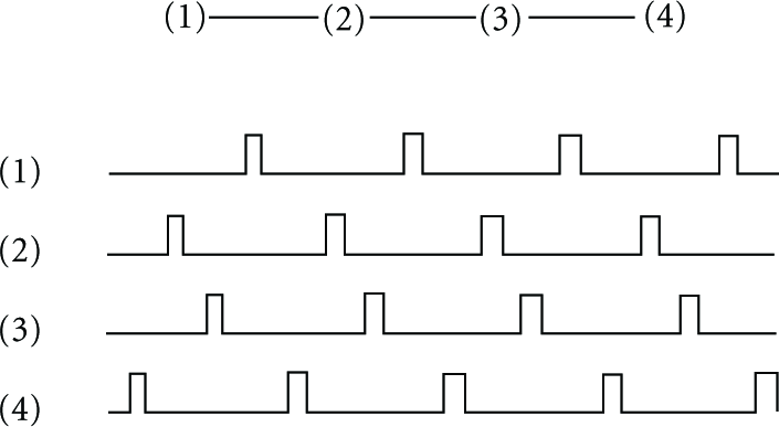
An uncoordinated node schedule.

Some MAC protocols arrange to have nodes occasionally sample radio activity during sleeping periods, with the aim of learning what other nodes are in the vicinity and what are their schedules; the appendix cites papers on low-power MAC protocols for WSNs that use sampling. These sampling techniques depend on a radio feature for channel sampling that is fast and consumes very little power. By contrast, the discovery protocols surveyed in Section 5 do not depend on extra radio features. If sampled neighboring node schedules are predictable (i.e., periodic), then some additional waking time can be scheduled. Figure 2 shows a modification to the scenario of Figure 1 in which node (3) has learned the schedules of (2) and (4), and then added to its waking times to facilitate communication. Note that in addition to enlarging its waking time to accommodate (2) and (4), node (3) retains its original schedule as well, in case any other nodes that have learned about (3) depend on its schedule.

Figure 2

Node (3) accommodates its neighbors.

Does learning of neighboring nodes then accommodating their schedules solve the problem of neighbor discovery? Yes, however, one would hope to have a power-optimal solution to neighbor discovery rather than adding additional waking times to accommodate neighbor schedules. Remarkably, protocols (surveyed in Section 5), by careful arrangement of their schedules, are able to learn of neighbors without extra sampling of the radio during their sleeping periods. It should be possible for a WSN to overcome improper initialization or ad hoc network formation, so that eventually all schedules are coordinated, as shown in Figure 3. Having all nodes move to a common, coordinated schedule (analogous to TDMA) will result in lower power consumption.

Figure 3

Coordinated node schedule.

For more traditional, mobile ad hoc networks (MANETs) where power conservation is not so critical, neighbor discovery is the simpler problem of continuously detecting that mobile stations come into range—converging to a common schedule like that shown in Figure 3 is not important. Many WSN applications are either event-driven (and nodes cannot wait long to transmit data) or the power requirements are not so stringent. For these applications, learning of and accommodating to neighbor schedules is adequate.

3. Wakeup in Distributed Systems

A sensor node saves power by turning off its radio. While the radio is off, that sensor neither receives messages nor responds to queries or commands. It is dormant as far as other nodes in range of communication are concerned. We thus say that a node is asleep when its radio is off, and awake when the radio is on. Two nodes are (communication) neighbors if they can communicate when both are awake.

Results from the WSN literature on neighbor discovery explore arbitrary communication topologies that have bidirectional communication links. That is, if p and q are neighbors, then p can hear q's messages and vice versa; in reality, the neighbor relation could be asymmetric, so that p could hear from q, whereas q would be unable to receive from p presentation. In WSN deployments, it could be possible that a link is asymmetric; the papers surveyed in this paper generally presume bidirectional links. The assumption of symmetry simplifies analysis and protocol research. In our opinion, neighbor discovery with unidirectional links is an open problem. We suggest in Section 7 some considerations regarding unidirectional links in research. Note, however, if a network can be connected using bidirectional links, then unidirectional links could be ignored or discarded for routing or other applications; whether or not the case of unidirectional communication really matters depends on empirical properties of WSNs in practice.

Other simplifying assumptions about timing are introduced later in the article. Generally, we shall ignore the possibility of failures, including message corruption, radio interference, and frame collision during transmission. Because discovery is an ongoing protocol, engineered to cope with dynamic, ad hoc WSNs, the consequence of simplyfing assumptions is that the latency for discovery is prolonged by communication failures. So long as communication succeeds with sufficient probability, discovery eventually occurs. Even when more realistic models are used, the techniques and themes surveyed in this article would be valid starting points for design and implementation of neighbor discovery protocols.

The neighbor discovery problem has a trivial solution if nodes are given the ability to “wake up” sleeping neighbors. It is common in wired local area networks to have a special wakeup command, which causes sleeping nodes to become awake. This feature turns out to be difficult or prohibitively expensive for sensor nodes at the current level of technology. There is one commonly used exception, passive RFID technology, where nodes receive not only a message but also the power needed to compute and respond, from an electromagnetic signal. Limitations on range and the power needed for signaling (plus the cost of extra components) rule this option out for WSN deployments, so the trivial solution of transmitting a wakeup command and hearing acknowledgments is not considered to be a satisfactory neighbor discovery protocol. However, wakeup considered in a broader context is sufficiently important, yielding many interesting and relevant techniques, as mentioned briefly in the following paragraphs.

Among the well-studied problems for distributed algorithms are variants of the wakeup problem. Perhaps the oldest of these is the firing squad problem [1]: a multihop network is given with all nodes initially asleep; one node is selected to spontaneously wake up, and the goal is to have all nodes perform some action only once, and simultaneously. Algorithms for this task thus rely on the initiator node sending messages to neighbors, which are propagated to their neighbors, and so on, to wake up the entire network; superimposed on this wakeup scheme, there needs to be a timing strategy so that nodes only perform the desired action at the same instant all their neighbors do (transitively, the entire network). Metrics for optimization include the number of messages, the size of messages, the latency period between initial activation and the firing of the action, and the overhead (memory, program size) of the algorithm. Obviously, a sleeping node cannot know when the initiator will wake up, and this resembles one of the fundamental difficulties of the neighbor discovery problem: a node cannot know (except for very specific deployments) when another node enters into its neighborhood and is capable of being awake.

Theoretical study of wakeup in a shared communication medium network starts with [2]. The network there is single-hop (i.e., a clique topology) and messages are unicast, unlike the wireless model where a single message can be received by all neighbors. Despite such differences from the WSN model, an important observation is relevant to neighbor discovery in a sensor network: the timing of when a node sends a message (or engages in some higher-layer multicast protocol) is important. The schedule of transmitting messages can be deterministic or random, and the choice of a schedule is crucial to efficiency. One schedule described in [2] gives each node in the system a different schedule, based on periodically transmitting after some silent period. The length of the period is chosen to be a prime number so that each node has a different prime, and this turns out to guarantee certain synchronization properties. We will see in Section 5.4 that such a technique has been exploited in several investigations of the neighbor discovery problem.

Another perspective on discovery, again from the literature of distributed computing, is found in [3], which shows how to match up servers and clients in a distributed, message-passing system. With n servers and n clients, it turns out that $O (\sqrt{n})$ messages suffice to guarantee a fully distributed rendez-vous between matching parties (a nondistributed solution would be to have one leader node coordinate all of the matching, but it then becomes a single point of failure or contention). The idea is based on an $n \times n$ matrix, with rows representing servers and columns representing clients. The server of row i tells a set of $P (i)$ nodes about itself, whereas the client of column j queries a set of $Q (j)$ nodes for the desired service. Then, by arranging P, Q so that $P (i) \cap Q (j)$ is nonempty, discovery will occur. It turns out that $| P (i) | = ⌈ \sqrt{n} ⌉$ and $| Q (i) | = ⌈ \sqrt{n} ⌉$ effectively load balances the match-making process: a lower bound of $Ω (\sqrt{n})$ is shown in [3] on the average message complexity for discovery between client and server. The view of discovery through a matrix or table with rows and columns representing different parties occurs in the WSN neighbor discovery literature (see intersecting designs in Section 5.3). An earlier reference to such a problem can also be found in the seminal paper [4] on replica control in databases; later, a more sophisticated construction [5] was discovered for mutual exclusion, which achieves $O (\sqrt{n})$ complexity, n being the number of nodes (incidentally, the initial construction depends on finding a prime factor to establish the existence of a particular subset of nodes that guarantee rendez-vous). Finding special arrangements of awake times, rather than node locations, turns out to be similar and useful for neighbor discovery.

4. Platform

This section briefly introduces terminology and facts about sensor nodes used later in descriptions of protocols. More detail on platform issues can be found in the appendix. Most of the protocols are based on discrete models of time and communication, so a slotted model of time is a reasonable discipline for protocols and a convenient analysis abstraction. The appendix discusses some of the concerns of the slot abstraction as well as duty cycle, processor, clock, and radio facilities relevant to neighbor discovery.

The Slot Model

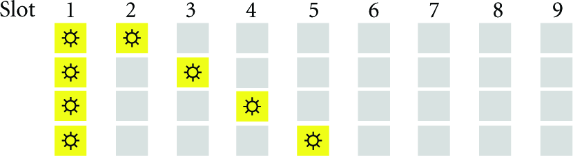
Before delving into the details of protocols, it is helpful to explain some terminology found in the literature of neighbor discovery. Time is modeled in discrete units called slots, which are supposed to be intervals of real time of sufficient length to permit communication. A node can either be awake or asleep in any given slot. Discovery protocols use schedules of awake and asleep intervals, most of them based on slots, with the objective of keeping the ratio of awake slots to total slots to a suitably low duty cycle (see appendix for details and motivation of duty cycles). During operation, we can refer to a node's current slot by some fictional counter value, so that a protocol or schedule may be concisely described. For convenience of presentation and analysis, we further suppose that all nodes commence and terminate their slots in unison: a trace of a WSN execution is thereby depicted by a diagram in Figure 4 where rows are nodes, slot numbers increase left to right, and the starting points for all slots line up vertically. Given such an ideal arrangement of slotted time, the basis for neighbor discovery is easy to define. If p and q are neighbors who have not yet discovered each other, and if they are awake concurrently in some slot k, then they discover each other and the fact of this discovery is retained for slots $k + 1$ and higher. We call the event of p and q discovering each other mutual recognition.

Slots are a convenient abstraction, though time on WSN platforms is not inherently divided into slots. Nodes can approximate being awake and asleep for intervals that would approximate multiples of slot length; also, nodes cannot be expected to have their slots precisely aligned as Figure 4 shows. Assume that a slot is the minimum-length time interval for two nodes to exchange messages, thus adequate for mutual recognition; that is, if neighbors are both awake for the duration of one slot, then each neighbor receives some message from the other. While it would be ideal for nodes to discover each other in one slot time, it is quite improbable in practice that that neighbors would have slots so precisely aligned, starting their slots simultaneously. Therefore, implementations of these slotted protocols may stretch the length of the awake interval, aiming for sufficient overlap even when the slots are not aligned. To see this, consider an awake interval comprising three slots, that is, three times the minimum-length time needed for mutual recognition.

Figure 5 shows awake periods for two nodes, (1) and (2), which do not have aligned slots. Because each interval's length comprises three slots, a sufficient condition is that these two awake intervals satisfy: the center slots of each have some (even small) overlap. That condition guarantees that the two intervals overlap by at least the duration of one slot, indicated, for instance, by the dotted vertical lines in the figure. The condition suggests an approach to designing a neighbor discovery protocol. First, assume that slots are aligned; then design a protocol that guarantees, neighbors eventually are both awake during some slot (the subject of Section 5). Second, when implementing this protocol, prefix any scheduled contiguous sequence of awake slots with one extra awake slot, and similarly add a suffix of one extra awake slot to the sequence. The idea from Figure 5 then overcomes the fact that slots are not aligned in practice. Thus the consequence of using simplistic model of aligned slots is that neighbor discovery protocol results, presented in later sections, will be degraded by some (hopefully constant) factor in an implementation of the protocol. Further motivations for extending the awake periods (due to collisions and other phenomena) are discussed in the appendix. The work of [6] suggests another way to deal with unaligned slots: at the start and end of each slot, a beacon is transmitted, which is enough to trigger discovery. The implementation findings reported in [6] using the slot abstraction state that only in 2% of cases did the actual discovery time exceed that predicted by analysis and simulation based on aligned slots.

Figure 4

Slots for p and q. ☼ denotes awake.

Figure 5

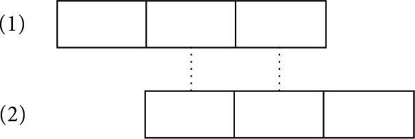
Unaligned slot sequences.

5. Protocols

Protocols for neighbor discovery exploit three basic themes, though a variety of constructions combine the themes and emphasize them differently. First, a sensor node can use randomness to influence behavior. Random choice of which slots are awake or sleeping is a probabilistic method of obtaining mutual recognition. Second, there are patterns of awake slots that guarantee neighbor discovery when all nodes use them. Third, a node can remain awake for a number of consecutive slots to assure neighbor discovery.

Whatever the technique used for obtaining discovery, an important question is what should be done after discovery? Most papers gloss over this question, though it deserves some explanation. Suppose that neighbors p and q achieve mutual recognition in some slot at time t. One design choice would be for both p and q to record the fact of a new neighbor in local state variables and then continue with the discovery protocol after time t, each perhaps discovering other neighbors. If the discovery protocol also exchanges some extra information, then with each discovery a node may also obtain the schedule for each neighbor. Thus, node p would have a table of its neighbors and their sleeping schedules. A different design choice would be for nodes to change behavior following the event of neighbor discovery. Thus, at time t when p and q discover each other, at least one of the two nodes changes its sleeping schedule so that thereafter p and q have identical sleeping schedules. We call this a merge event. If two nodes merge, at least one of them switches its sleeping schedule (or changes its current slot number within the schedule). While this may seem simple, it can be more involved after a history of merge events: perhaps two connected components A and B each contain multiple nodes, that is, $| A | > 1$ and $| B | > 1$ . Now if a node in $p \in A$ and a node in $q \in B$ discover each other, how should a merge event proceed? If p is to adopt q's schedule, then does p “move” from A to B, or should all nodes of A and B merge into one schedule? The latter choice would imply some kind of distributed algorithm to effect the schedule change, which is problematic for a low duty-cycle WSN application. We leave the details of merging questions open in this article, due to the lack of literature on this topic.

Some WSN applications make use of the radio's local broadcast ability: with one transmission, a node can send data to all its neighbors. If this feature is desired, then a merging protocol is superior to a nonmerging protocol, because after merging, all neighbors would be awake to receive a local broadcast (because they would have the same sleeping and awake schedules). For applications that use only unicast, a non-merging protocol could be sensible. A hybrid of these two approaches would be a discovery protocol for single-use deployments, where nodes engage in non-merging neighbor discovery for some fixed time period, and then all nodes switch to a common sleep schedule.

5.1. The Birthday Protocol

The idea of the birthday protocol is dual to the randomization strategy behind CSMA/CA in 802.15.4 for sensor networks. Recall that for CSMA/CA, a node delays for some random interval before attempting transmission. The purpose of delay is to increase the probability of finding a transmission time that avoids collision, that is, neighbors do not transmit simultaneously. In contrast, the goal of the birthday protocol is to use random selection between awake and sleeping states so that neighbors are awake simultaneously. The work of [7] proposed the birthday protocol for low-power communication, based on transitions between three node states. Entering a state amounts to starting either an asleep or awake interval of fixed duration, which is effectively a slot. At the start of each slot, a node chooses with probability $p_{s}$ , $p_{t}$ , and $p_{ℓ}$ whether the state for that slot is to be sleeping, transmitting, or listening. During a transmitting slot, a node broadcasts a discovery message. The work of [7] refines this approach further by arranging for nodes to have different modes, using timing parameters tuned for performance, which tune the frequency of entering a transmitting state.

A notable feature of the birthday protocol is that it does not require neighbor discovery as such. (Though [7] is oriented to neighbor discovery, we observe that it could directly be used as a MAC protocol in which nodes may sleep.) Nodes could use this protocol to send and receive messages, without needing any particular sleeping schedule, because the duration of sleeping is a random variable. An open question is how nodes should behave in birthday protocol following discovery—the argument of the authors of [7] is that the birthday protocol can be memoryless, with no durable consequences of discovering a neighbor. In contrast, other papers [7] as a discovery mechanism do suggest that discovering a neighbor could modify subsequent protocol behavior. We thus consider as an open problem how the randomized technique of the birthday protocol could be used for more durable discovery and scheduling. It seems that merging would be possible, though the behavior of a merged set of nodes should be the same with respect to random choices after the merge. That is, when nodes merge, they should adopt a common seed for a pseudorandom number generator, so that they coordinate sleeping.

Analysis of the essential ideas of the birthday protocol appears in [8, 9] for a 1-hop network (fully connected) with application to ad hoc networks. We did not find analytic results on the birthday protocol for multihop networks. Analysis in [9] derives a time period after which, with high probability, all neighbor discovery is completed (this assumes that all nodes start at approximately the same time). Analysis in [8] compares the energy cost of the simple birthday protocol, of the kind outlined here, to a round-robin birthday protocol.

5.2. Brute Force

The simplest deterministic protocol for neighbor discovery is the periodic schedule of n slots, with the first $⌈ (n + 1) / 2 ⌉$ of these being awake and the remaining slots for sleeping. This can informally be called the “51%” solution, since the idea is to remain on for slightly more than half of a period. No matter how two neighbors are initially offset in where their periods begin, mutual recognition is assured because their awake intervals must overlap. Several papers either explicitly or implicitly use this brute force technique or similar [10– 12]. Let the periodic interval of n slots be called a round. Clearly, neighbors discover each other within one round, which is optimal in terms of the latency of the discovery process. Unfortunately, the duty cycle is at least 50%, which is unacceptable for low-power operation.

A method of reducing the duty cycle below 51% is proposed in [10, 12]. Let $k = ⌈ (n + 1) / 2 ⌉ - 1$ and consider a logical division of the initial $⌈ (n + 1) / 2 ⌉$ awake slots into the first slot and the k subsequent slots. Suppose that r is a divisor of k. Now partition the k slots that follow the first slot of the round into r sequences, labeled $f_{0}, f_{1}, \dots, f_{r - 1}$ . Each interval $f_{i}$ consists of r consecutive slots. With this terminology, we consider a transformation of the 51% solution by letting each round begin with one awake slot, but distributing the intervals $f_{i}$ over r rounds. For example, if $r = 2$ , there are two intervals $f_{0}$ and $f_{1}$ , each having $k / 2$ slots, spread over two rounds: in the first round, we have $1 + k / 2$ awake slots followed by $n - (1 + k / 2)$ sleeping slots; in the second round, there is one awake slot followed by $k / 2$ sleeping slots, then $k / 2$ awake slots, and $n - (1 + k)$ sleeping slots. The schedule for a node is to repeat the pattern of these two rounds. Observe that, except for their first slots, the awake times of the first and second rounds are disjoint.

Figure 6 illustrates an example where $n = 9$ , $k = 4$ , and $r = 1$ , which produces a sequence of four rounds. The figure shows the four rounds as rows of a table, with columns representing slots. The symbol ☼ indicates that a slot is awake. The duty cycle for this schedule is less than half of the 51% approach, $2 / 9$ . To get some intuition why this translation of brute force into multiple rounds is valid, consider two neighbors p and q that have an offset of six slots and the following scenario. Node p starts with the first round at time 0, and node q starts at time 6 with the first round (time and slot numbers are synonymous here). Thus p is awake at times 0 and 1, then asleep until time 9, when its second round begins. Following the patterns of rows for Figure 6 awake times for p are 0, 1, 9, 11, 18, 20, 27, 31, 36, and 37. Node q is awake at times 6 and 7, then asleep until time 15. The awake times for q include 6, 7, 15, 17, 24, 26, 33, 37, 42, and 43. We see that both p and q are awake at time 37, which suffices for discovery. The rationale for the pattern is seen from the table. The “union” of relative awake times for the four rows is the 51% schedule.

Figure 6

Brute force transformed to lower duty cycle.

The translation of brute force to a scheme that spreads awake slots over time does reduce duty cycle, but at a cost: the time needed to guarantee discovery is larger: the discovery time is in the worst case r times greater (see analysis in [10]). This translation partitions a consecutive sequence of slots into an interrupted, irregular pattern of waking and sleeping. In many of the other discovery protocols we see a similar idea, where an irregular sleep pattern is used to obtain low duty cycle. Depending on application constraints, an irregular sleep pattern may not be useful for the application's tasks of sensing, computing, and communicating. At least the first slot of each round in the transformed brute force approach occurs periodically. A hybrid adaptation of the idea, combining the translation and randomized selection, would be a schedule with two awake slots, one at the start of each round and the other randomly selected from the remaining slots in the round.

A different method to reduce the duty cycle, again based on the brute force technique, is used in [11]. The basis for their method is to have one awake slot at the start of every round; however this is augmented by sometimes using the 51% solution in a round. For example, once every n rounds, a node is awake during $⌈ (n + 1) / 2 ⌉$ consecutive slots, this achieves a $2 / n$ duty round, at the cost of increasing the worst-case discovery time of the protocol. Because a node would need to be awake for $n / 2$ consecutive slots, this method might be unsuited to energy-harvesting platforms.

5.3. Intersecting Designs

Finding schedules of awake and sleeping slots to guarantee neighbor discovery has a combinatorial interpretation. The problem is to devise schedules with minimum duty cycle that are self-intersecting with respect to any rotation. Suppose that π denotes the indices of awake slots in an n-slot round. An example of this for $n = 16$ is $π = {0,3, 4,12}$ . A k-rotation of π is obtained by adding k to each index, modulo n, denoted by $π^{k}$ . Thus the 5-rotation of the example produces ${5,8, 9,2}$ . The combinatorial task is to find minimum size π such that $π \cap π^{k} \neq \emptyset$ for $0 \leq k < n$ . Finding such a sequence readily provides a schedule so that no matter how neighbors are offset, a common awake slot is guaranteed within a complete round.

While self-intersection for any k-rotation yields discovery within a round, the neighbor discovery problem in general does not require discovery within one round. Depending on how important discovery is to the application, weaker combinatorial problems, perhaps asking for intersection over a history of rounds, would be satisfactory. The results surveyed in this subsection target guaranteed discovery within one complete round. Also, note that the problem of finding self-intersecting sequences need not be restricted to all nodes using the same sequence. We may distinguish between symmetric solutions, where all nodes use the same sequence, and asymmetric solutions where nodes use different sequences from a set 𝒮 of patterns, such that any $S \in 𝒮$ is guaranteed intersection with $T^{k}$ for $T \in 𝒮$ . We concentrate first on symmetric solutions and return in the next subsection to asymmetric solutions.

Lower bounds on the number of awake slots needed for self-intersection are explored in [13, 14]. The problem requires $Ω (\sqrt{n})$ slots to be awake for discovery. In effect, the solution schedules with $O (\sqrt{n})$ awake slots correspond to the match-making work cited in Section 3. The schemes proposed in [13] are combinatorial designs, which have other applications in discrete mathematics. However, the first paper to explore such schedules for discovery is [15], which used the quorum idea, similar to the work of [5] on mutual exclusion. The works of [13, 14] improve on the quorum construction with lower power and considering multihop topologies and investigating randomized schedules with high probability of self-intersection with rotation.

Designs based on self-intersecting schedules are chiefly of interest to applications that need to minimize discovery latency, while also minimizing power usage. Whereas the brute force approach has a duty cycle of at least 1/2 to minimize latency, the existence of self-intersecting schedules would argue that power can be substantially reduced. However, there are some considerations for using these schedules with low duty cycles. Suppose that a 0.1% duty cycle is needed, and ignore constants in the $O (\sqrt{n})$ bound, for estimation purposes. To obtain the 0.1% duty cycle, we require $\sqrt{n} / n = 1 / 1000$ ; hence $n = 1 0^{6}$ . A deterministic self-intersecting schedule could impose some complex representation challenges for software implementation, depending on platform resource. Also, the schedule will be irregular, which may not be compatible with desired application behavior. Finally, the platform typically puts a practical lower bound on the duration of a slot, typically in tens to hundreds of milliseconds: the duration of a round, and therefore worst-case discovery time, will be on the order of several hours. (This last observation merely illustrates that there is a tradeoff between low duty cycle and discovery latency.)

5.4. Coprime Schedules

The last type of protocol we survey is based on periodic rounds that have relatively prime length with respect to neighbors, reprising an idea mentioned in Section 3. Thanks to the Chinese Remainder Theorem [16] if neighbors p and q have rounds in which the first slot is awake and the rest sleeping, and the two round lengths are relatively prime, then discovery is guaranteed. Put more formally, let $c_{p}$ and $c_{q}$ be the respective number of slots in the rounds of p and q. Numbers $c_{p}$ and $c_{q}$ are coprime if their greatest common divisor is 1. The latency for mutual recognition is, in the worst case over any offset between the two rounds, $c_{p} \cdot c_{q}$ .

Several observations concerning coprime schedules affect its suitability for WSN deployments. First, nodes need individualized programs so that each node has a round length coprime to all its neighbors. This can be done by assigning each node its own prime number; however this adds to deployment cost (and may be error-prone). Second, the duty cycle for a schedule of $c_{p}$ rounds is $1 / c_{p}$ ; if different primes are used, the asymmetry of different duty-cycle rounds in the network will depend on the set of primes chosen (though, after fully merging, all nodes could use a common round). Third, the schedule's arrangement of periodic rounds with one awake slot is a good fit for applications performing periodic sampling, perhaps by extending the one awake slot to an awake interval of slots. Note that in coprime scheduling we see a tradeoff between latency and duty cycle: lower latency is obtained by using smaller primes, but this entails higher duty cycle.

Several papers propose coprime scheduling for neighbor discovery [6, 10, 11], using different techniques that deal with the possibility that neighbors were given the same prime number for their rounds. The choice of a prime can be dynamic, by random selection. That enough does not ensure that neighbor rounds have coprime length, because there remains the possibility of unlucky random choices that deal with the same prime to a pair of neighbors. The technique proposed in [10] is to repeat the random prime selection process. For example, p may start with a randomly selected $c_{p}$ , use that for $k \cdot c_{p}$ rounds, and then choose again randomly another prime value for $c_{p}$ . The value k can be tuned, and random selection is confined to a set of two coprime numbers ${z, z + 1}$ to get an expected discovery latency in $O (z^{2})$ slots. Two deterministic approaches are investigated in [6, 11]. The idea of [6] is to assign a pair of primes ${c_{p}, d_{p}}$ to any node p. The sleeping schedule is modified so that a slot t is awake when either $t \mod c_{p}$ or $t \mod d_{p}$ is zero. Because $c_{p} \neq d_{p}$ , even if neighbors have the same pair of primes, discovery is assured. Tuning the selection of primes for a desired duty cycle, and a refinement using a triple of primes per node is also proposed in [6]. An advantage of multiple primes is that duty cycles can be adjusted at finer grain, because the duty cycle is approximately $1 / c_{p} + 1 / d_{p}$ ; moreover, different nodes can have distinct duty cycles, if an asymmetric schedule is useful to the application. The remaining technique, proposed in [11], to overcome using the same prime at different nodes is the one mentioned at the end of Section 5.2 proposed (a transform of brute force) where one in every $c_{p}$ rounds is a round with the 51% solution.

6. Metrics

Two criteria for evaluating a neighbor discovery protocol are latency and duty cycle. Latency is informally the time taken to discover a neighbor. Formally, latency can be measured in several ways: (i) the {mean, median, maximum} times for two neighbors to mutually recognize, taken over all nodes and all initial configurations (of offsets and protocol parameters, such as prime number assignments) between the nodes; (ii) the mean time for a node to discover all its neighbors, taken over different offsets, nodes, and topologies; and (iii) the mean and maximum time to “termination”, that is, when all nodes have discovered all their neighbors, again taken over all initial conditions and protocol parameters. In addition to these systemic questions of latency, one could ask about time taken for a new node added to a network, or a topology change, to be recognized. We focus on latency in this section, particularly the worst case and distributions of discovery times.

The work of [11] starts with the observation that, for certain worst-case latencies in the class of deterministic protocols, the characteristics of optimal schedules, with respect to the number of awake slots, were shown in [13]. An optimal schedule's number of awake slots can be used as a benchmark for evaluating different protocols. The authors of [11] propose that a combined metric, the power-latency product, be a basis for comparison. Their analysis for power-latency product shows that the quorum protocol [15] and the pair-of-primes protocol [6] are at least a factor of two greater than the optimum, whereas the single prime protocol of [11] is a factor 3/2 greater than the optimum. Another paper [12] suggests that randomizing the choice of which slot is awake (in the transform at the end of Section 5.2) may have better mean time to discovery than [11].

Is the power-latency product a good target for optimization? When either factor, time to discovery, or duty cycle is held constant, the other factor indeed should be minimized. The attractiveness of the power latency product is its neutrality with respect to tradeoffs for the several protocols surveyed: if latency is to be reduced, using several of the techniques explained in this article, it is at the cost of increased power utilization (for an optimal protocol), due to higher frequency of scheduled awake slots. If these two factors are commensurate, then tuning latency does not change the metric. Power-latency as a metric is similar to the delay-power product for design of switching circuits, where higher power can be necessary for faster response. One aspect missed in the power-latency comparisons in [11] is the distribution of discovery latency times, rather than comparing by analysis of the worst-case latency.

6.1. Simulations

The performance behavior of discovery has been evaluated in [6, 11] by simulation and implementations. The Disco paper [6] explores several questions by simulation, but left open the issue of how discovery times are distributed. To better understand how protocols surveyed in Section 5 compare with respect to discovery time distribution, we simulated them. While a number of sensor network simulators are available, for instance, [17, 18], these tools simulate protocols at a low level. How discovery times are distributed is a simpler question, readily answered by a discrete event simulator; we wrote a small simulator in Python for our investigation.

The simulator was constructed as follows. One iteration of the simulator runs a given discovery protocol on a fixed number of immobile nodes from a start state in which nodes have freshly generated random offsets to an end state in which all edges have been discovered. Each protocol evaluated was run through 1000 simulator iterations; the time at which each edge was discovered was recorded. For this set of simulations, we fixed the duty cycle to be approximately 1% on a clique topology of 48 nodes (for those protocols that could not realize a duty cycle of 1% a slightly lower approximation was used). For all the protocols, we chose parameters to get symmetric behavior (the same duty cycles), meaning that we chose a single prime for all nodes for protocol [11] and drew each prime randomly from a set of four candidate primes to simulate Disco [6], following the authors advice to choose for each node one prime near the reciprocal of the duty cycle (100 for the 1% duty cycle) and a second, larger prime to create a duty cycle closer to 1% (e.g., a valid 1% duty cycle prime pair would be (101, 10103)). To achieve the 1% duty cycle for the 51% solution, we used the transformation of one extra slot per round explained in Section 5.2. The initial state of a node, that is, where the node started the simulation with respect to the slot schedule of awake/asleep, was uniformly random for each of the 48 nodes. The resulting edge discovery times, totaled over the 1000 iterations, were then grouped into buckets (each representing 100 consecutive slot times); each bucket is a point in the graph, and lines through the points show the distribution of discovery counts on the y-axis versus slot times on the x-axis. Note that these simulations do not use any kind of merging strategy—each node adheres to its schedule throughout the simulation.

Figure 7 shows the results. The results show how different protocols exhibit different discovery time distributions. Deterministic approaches, quorum and the 51% protocol, end at a certain slot for all simulation runs (this ending slot represents the worst case). The Birthday protocol's distribution confirms the classical combinatoric distribution one would expect (which can be analytically predicted by probability theory). The long tail on Disco is due to the effect of large primes, explained here in after.

Figure 7

Discovery time distributions from simulation.

The 51% protocol differs from the other deterministic protocols by its discovery occurring at a relatively constant rate. This protocol's neighbor-discovery time is directly proportional to the relative initial offset between neighbors. Since the relative offsets are uniformly distributed initially, the discovery times are uniformly distributed (up to the worst case).

The distribution of [11] is relatively flat because all nodes use the same prime number for their schedules. Recall from Section 5 that a node is awake once every p slots (p being the prime), but after $p - 1$ such iterations are awake for $p / 2 + 1$ slots. Hence, a node is awake for short intervals frequently and long intervals infrequently. Due to the uniform distribution of initial states and offsets, the long intervals are uniformly distributed over the simulation. In such a simulation, discovery only occurs when a long interval is involved, hence the distribution follows a flat curve. (We also ran simulations of [11] with many distinct primes, and the resulting distribution had a pronounced downward slope, reflecting the diversity of opportunities for discovery, which reduced over time.)

The Disco distribution [6] shows larger discovery rate in the beginning; the protocol gives an advantage to neighbors with distinct smaller primes. Over the course of the simulation, neighbors with smaller primes are simultaneously awake in numerous slots; however, we only count the first such slot for discovery. Hence, we see more discoveries toward the start of a simulation than later. After the edges discovered through such intersections (driven by smaller primes) are exhausted, we then see the distribution drop to a long tail. In the long tail, neighbors get mutual recognition during a slot governed by at least one larger prime. The distribution's flat long tail is explained by realizing that both of neighboring node's prime pairs and offsets are assigned randomly; once the choice of (large) primes and offset is set at the initial state, the distribution of meeting times between distinct large primes tends to be uniform over the simulation.

Note that the Quorum protocol's distribution is roughly linear, and the downward slope appears to be the same as the initial part of the Disco distribution. The explanation is the same: over the course of the simulation, a given pair of neighbors $(p, q)$ are awake simulataneously at numerous times. The simulation only counts the first intersection of $(p, q)$ for discovery; the total number of opportunities for edge discovery diminishes over time until all edges are discovered.

7. Conclusion

This article collected the ideas prevalent in recent literature on the neighbor discovery problem for wireless sensor networks. The basic methods of randomization and combinatorial sequences appear in several papers, with the most recent papers beginning deeper, hybrid constructions for neighbor discovery. One technique not yet fully explored could be sharing of discovery information with neighbors. If p and q have discovered each other, and then p discovers r, there is some probability that r is also a neighbor of q, and this could be exploited to accelerate a $(q, r)$ discovery. Generally, heuristics suitable to particular topologies or neighbor densities have not been explored in the literature.

In Section 3 it was observed that the case of unidirectional links in neighbor discovery is not explicitly researched in the papers we have surveyed. To give the reader some idea of the considerations involved, suppose that the simple linear topology of Figure 1 is unidirectional, where node (1) cannot receive from any other node, (2) only hears from (1), (3) only hears from (2), and (4) can only receive from (3). In principle, it should be possible for each node except (1) to learn of the upstream neighbor and adapt its schedule accordingly; as a result, all nodes may eventually adopt the schedule of (1). The case of a cyclic network topology with unidirectional links would be more challenging, apparently requiring some way to break symmetry. These considerations suggest that complete solutions to the case of unidirectional communication could be complex and perhaps unsuited to the simple sensor network platforms.

Though protocols surveyed in Section 5 can work for multihop WSNs, we did not find analysis or extensive measurements of behavior for the multihop case. The issue of merging after discovery, relatively simple for a single-hop network, becomes more intricate for multihop networks.

Only two of the papers surveyed [6, 11] report empirical work with implementation. Further practical experience would be most helpful to prioritize research issues in this area. The case study reported in [11] implemented neighbor discovery in the FireFly Badge platform, used in the Sensor Andrew project [19]. The platform was embedded into a key-chain form factor and then used to support a social networking application.

Footnotes

Appendix

References

Moore

E. F.

Moore

E. F.

The firing squad synchronization problem

Sequential Machines 1964

Addison-Wesley

213 214

Gasieniec

Pelc

Peleg

Wakeup problem in synchronous broadcast systems

Proceedings of the 19th Annual ACM Symposium on Principles of Distributed Computing (PODC ’00)

2000

113 121

Mullender

S. J.

Vitányi

P. M. B.

Distributed match-making

Algorithmica 1988 3 1 367 391

2-s2.0-0023828361

10.1007/BF01762123

Gifford

D. K.

Weighted voting for replicated data

Proceedings of the 7th ACMSymposium on Operating Systems Principles (SOSP ’79)

1979

150 162

Maekawa

\sqrt{N}

algorithm for mutual exclusion in a decentralized systems

ACM Transactions on Computer Systems 1985 3 2 145 159

2-s2.0-0022069122

Dutta

Culler

Practical asynchronous neighbor discovery and rendezvous for mobilesensing applications

Proceedings of the 6th International Conference on EmbeddedNetworked Sensor Systems (SenSys ’08)

2008

71 84

McGlynn

M. J.

Borbash

S. A.

Birthday protocols for low energy deployment and flexible neighbor discovery in ad hoc wireless networks

Proceedings of the 2nd ACM Interational Symposium on Mobile Ad Hoc Networking and Computing (MobiHoc ’01)

October 2001

137 145

2-s2.0-0035789555

Fang

Berber

S. M.

Swain

A. K.

Analysis of neighbor discovery protocols for energy distribution estimations in wireless sensor networks

Proceedings of the IEEE International Conference on Communications (ICC ’08)

2008

4386 4390

10.1109/ICC.2008.823

Vasudevan

Towsley

Goeckel

Khalili

Neighbor discovery in wireless networks and the coupon collector's problem

Proceedings of the 15th Annual International Conference on Mobile Computing and Networking (MOBICOM ’09)

September 2009

181 192

2-s2.0-70450235097

10.1145/1614320.1614341

10.

Herman

Pemmaraju

Pilard

Mjelde

Temporal partition in sensor networks

Stabilization, Safety, and Security of Distributed Systems (SSS ’07) 2007 4838 Springer Lecture Notes in Computer Science

11.

Kandhalu

Lakshmanan

Rajkumar

U-connect: a low-latency energy-efficient asynchronous neighbor discovery protocol

Proceedings of the 9th International Conference on Information Processing in Sensor Networks (IPSN ’10)

April 2010

350 361

2-s2.0-77954488910

10.1145/1791212.1791253

12.

Bakht

Kravets

SearchLight: asynchronous neighbor discovery using systematicprobing

Mobile Computing and Communications Review 2010 14 4 31 33

13.

Zheng

Hou

J. C.

Sha

Asynchronous wakeup for ad hoc networks

Proceedings of the 4th ACM International Symposium on Mobile Ad Hoc Networking (MOBIHOC ’03)

June 2003

35 45

2-s2.0-0242612027

14.

Bradonjić

Kohler

Ostrovsky

Near-optimal radio use for wireless network synchronization

Algorithmic Aspects of Wireless Sensor Networks (ALGOSENSORS ’09) 2009 5804 15 28 Springer Lecture Notes in Computer Science

10.1007/978-3-642-05434-1_4

15.

Tseng

Y. C.

Hsu

C. S.

Hsieh

T. Y.

Power-saving protocols for IEEE 802.11-based multi-hop ad hoc networks

Proceedings of the 21st Annual Joint Conference of the IEEEComputer and Communication Society

2002

16.

Niven

Zuckerman

H. S.

Montgomery

H. L.

An Introduction to the Theory of Numbers 1991

New York, NY, USA

John Wiley & Sons

17.

Levis

Lee

Welsh

Culler

TOSSIM: accurate and scalable simulation of entire TinyOS applications

Proceedings of the 1st International Conference on Embedded Networked Sensor Systems (SenSys' 03)

November 2003

126 137

2-s2.0-18844399081

18.

Shnayder

Hempstead

Chen

B. R.

Allen

G. W.

Welsh

Simulating the power consumption of large-scale sensor network applications

Proceedings of the 2nd International Conference on Embedded Networked Sensor Systems (SenSys ’04)

November 2004

188 200

2-s2.0-26644435250

19.

Sensor Andrew http://www.ices.cmu.edu/censcir/sensor-andrew/

20.

nRF24 series data sheet, Nordic Semiconductor, http://www.nordicsemi.com

21.

CC2500 data sheet, Texas Instruments, http://www.ti.com

22.

CC2420 data sheet, Texas Instruments, http://www.ti.com

23.

MSP430 data sheets, Texas Instruments, http://www.ti.com

24.

ATMEGA128 data sheet, http://www.atmel.com

25.

Kohvakka

Suhonen

Kuorilehto

Kaseva

Hännikäinen

Hämäläinen

T. D.

Energy-efficient neighbor discovery protocol for mobile wireless sensor networks

Ad Hoc Networks 2009 7 1 24 41

2-s2.0-53549120933

10.1016/j.adhoc.2007.11.016

26.

Polastre

Hill

Culler

Versatile low power media access for wireless sensor networks

Proceedings of the 2nd International Conference on Embedded Networked Sensor Systems (SenSys ’04)

November 2004

95 107

2-s2.0-26444451023

27.

Silva

Heidemann

Ultra-low duty cycle MAC with scheduled channel polling

Proceedings of the 4th International Conference on Embedded Networked Sensor Systems (SenSys ’06)

November 2006

321 334

2-s2.0-34547398467

10.1145/1182807.1182839

28.

Hui

J. W.

Culler

The dynamic behavior of a data dissemination protocol for network programming at scale

Proceedings of the 2nd International Conference on EmbeddedNetworked Sensor Systems (SenSys ’04)

November 2004

81 94

2-s2.0-22744432612

Survey: Discovery in Wireless Sensor Networks

Abstract

1. Introduction

2. Motivating Scenario

3. Wakeup in Distributed Systems

4. Platform

The Slot Model

5. Protocols

5.1. The Birthday Protocol

5.2. Brute Force

5.3. Intersecting Designs

5.4. Coprime Schedules

6. Metrics

6.1. Simulations

7. Conclusion

Footnotes

Appendix

References