Sage Journals: Discover world-class research

Abstract

Many applications and protocols in wireless sensor networks need to know the locations of sensor nodes. A low-cost method to localize sensor nodes is to use received signal strength indication (RSSI) ranging technique together with the least-squares trilateration. However, the average localization error of this method is large due to the large ranging error of RSSI ranging technique. To reduce the average localization error, we propose a localization algorithm based on maximum a posteriori. This algorithm uses the Baye's formula to deduce the probability density of each sensor node's distribution in the target region from RSSI values. Then, each sensor node takes the point with the maximum probability density as its estimated location. Through simulation studies, we show that this algorithm outperforms the least-squares trilateration with respect to the average localization error.

1. Introduction

The process of determining the physical locations of sensor nodes is known as localization, which is a fundamental problem in wireless sensor networks [1, 2]. The locations of sensor nodes are essential in many applications and protocols. For example, the sensed information about an event without the location where it takes place is often meaningless. Similarly, geographic routing relies on the locations of nodes to forward packets [3].

The locations of sensor nodes can be directly obtained by preconfiguration or global positioning system (GPS). Preconfiguration requires each sensor node being placed at a known location, which is only suitable for the case that sensor nodes are easy to be placed and their number is small. On the other hand, a sensor node equipped with a GPS receiver is costly and does not work indoors. Therefore, both the above two methods are impractical for large-scale low-cost wireless sensor networks. It is desired that the locations of sensor nodes can be induced from their interactions, such as the detections of the distances between neighbors.

Many localization algorithms first use a ranging technique to estimate the Euclidean distances between nodes, and then use the least-squares trilateration to determine the locations of sensor nodes by these estimated distances. Some conventional ranging techniques are received signal strength indication (RSSI), time of arrival (TOA), time difference of arrival (TDOA), angle of arrival (AOA), and so forth [4]. Among them, RSSI ranging technique has the least requirement for hardware, as the radio chip of current sensor node usually has a built-in function of reading RSSI value. But RSSI value is vulnerable to being disturbed by the surrounding environment and the ranging error of RSSI ranging technique may be at most ±50% [5]. Furthermore, the least-squares trilateration is sensitive to ranging errors [2]. If using RSSI ranging technique together with the least-squares trilateration to localize sensor nodes, the average localization error is very large.

To reduce the average localization error, we propose a localization algorithm based on maximum a posteriori. This algorithm uses the probability approach to estimate the location of each sensor node directly from RSSI values. Extensive simulation results have shown that the average localization error of this algorithm is less than that of the least-squares trilateration.

The remainder of this paper is organized as follows. Related work is discussed in Section 2, the network model is defined in Section 3, and our proposed localization algorithm is described in Section 4. Simulation results that illustrate the performance are included in Section 5, and Section 6 is the conclusion.

2. Related Work

Since localization is a fundamental problem in wireless sensor networks, there are many research works focusing on it recently. Localization algorithms can be divided into two categories: anchor-based localization algorithms and nonanchor-based localization algorithms. An anchor is a special node which has a priori knowledge of its location.

In anchor-based localization algorithms, the location of each sensor node is determined only by its distances from anchors. Priyantha et al. developed the cricket location support system which provides localization services for indoor mobile node [6]. Bulusu et al. proposed a GPS-less localization algorithm in which each mobile node localizes itself to the centroid of its adjacent connecting anchors [7]. Niculescu and Nath proposed a family of distributed localization algorithms “adhoc positioning system” (APS) [8, 9]. In these algorithms, each node measures its distances from anchors by performing multihop propagation of distances to anchors throughout the network. Kumar et al. used RSSI-based weighted centroid to improve the localization algorithm proposed by Bulusu et al. [10]. Li and Liu proposed the rendered path (REP) protocol for locating nodes in anisotropic sensor networks with holes [11]. Lederer et al. also studied the problem of localizing a large sensor network having a complex shape, possibly with holes [12].

In nonanchor-based localization algorithms, the location of each sensor node is determined also by the distances between sensor nodes. Doherty et al. proposed a constraint-based localization scheme using semidefinite programming (SDP) to find a solution to the localization problem [13]. Shang et al. proposed an algorithm using classical multidimensional scaling (MDS) technique to calculate the locations of nodes given a set of distances [14]. Kwon et al. proposed a localization algorithm based on least square scaling (LSS) which is a variant of multidimensional scaling technique [15]. Khan et al. proposed a distributed iterative localization algorithm in m-dimensional Euclidean space with a minimal number of $m + 1$ anchors [16]. Ding et al. viewed localization as a (nearest) Euclidean distance matrix (EDM) completion problem and thus gave an EDM approach [17]. Zhu et al. used stress normal property to localize sensor nodes with enough perturbation data [18].

Many of the above-mentioned algorithms [12, 14, 15, 17] have a similar optimization objective as the least-squares trilateration, that is, minimizing the (weighted) sum of all squared differences between each estimated distance and the corresponding distance calculated by the estimated locations of nodes. But when the distances are estimated by RSSI ranging technique, this optimization objective is likely subject to a large average localization error. In this paper, we present another optimization objective with which sensor nodes can be localized more accurately.

3. Network Model

Before describing our proposed localization algorithm, we first assume the model of wireless sensor network as follows. (1)

A wireless sensor network is deployed in a planar region B. Suppose that B is a rectangle, whose length is l and width is w. But later we will see that the proposed algorithm is not dependent on the shape of B. Without loss of generality, we assume that the lower left corner of B is the origin and the coordinate of the upper-right corner of B is $(l, w)$ .

(2)

All sensor nodes are uniformly distributed in B. Anchors have a larger transmission range than sensor nodes. Each sensor node and anchor is denoted by a point in B. Let n denote the total number of anchors, $a_{i}$ denote the ith anchor, and ( $x_{i}, y_{i}$ ) denote the coordinate of $a_{i}$ .

(3)

Initially each anchor broadcasts a beacon containing its location information. Then, each sensor node collects the RSSI values of all its neighbor anchors through these beacons. The RSSI value read by a sensor node obeys the wide log-normal shadowing radio signal propagation model [19]:

\begin{matrix} R (d) = P_{T} - P L (d_{0}) - 10 η lo g_{10} \frac{d}{d_{0}} + X_{σ} . \end{matrix}

(1)

In (1), $R (d)$ denotes the RSSI value when the distance between the receiver and the transmitter is d; $P_{T}$ is the power of the transmitter; $P L (d_{0})$ is a known reference power value at a reference distance $d_{0}$ from the transmitter; η is the path loss exponent that measures the rate at which the RSSI value decreases with distance; $X_{σ}$ is a zero mean Gaussian distributed random variable with standard deviation and it accounts for the random effect of shadowing, that is, $X_{σ} = N (0, σ^{2})$ .

Given these known RSSI values, the locations of sensor nodes can be estimated by a localization algorithm. The major measurement of a localization algorithm is the average localization error, defined as the average distance between the actual location and the estimated location of each sensor node [5]. Because wireless sensor networks often work in unfriendly environments, some anchors may be faulty, which means they have incorrect information about their own locations. Therefore, fault tolerance is also important to a localization algorithm. In this paper, we define it as the ability to maintain a good localization result even if some anchors are faulty. Besides, execution time is also a common measurement of a localization algorithm.

4. Algorithm Description

In this section, we will describe our proposed localization algorithm based on maximum a posteriori. Consider a sensor node s. Let ( $x_{s}, y_{s}$ ) denote the coordinate of s and $r_{k}$ denote the random variable of the RSSI value of $a_{k}$ read by s, where $0 \leq k < n$ . Assume that the values of $r_{1}, r_{2}, \dots, r_{n}$ in a test are $R_{1}, R_{2}, \dots, R_{n}$ , respectively. The basic idea of our proposed localization algorithm is as follows. First, the target region B is divided into small grids of the same size. Next, the probability of s being in each grid is calculated from $R_{1}, R_{2}, \dots, R_{n}$ . Then, the center of the grid with the largest probability is taken as the estimated value of ( $x_{s}, y_{s}$ ). Let g denote the side length of each grid. Without loss of generality, assume that the target region B has exact $l / g$ grids in the horizontal direction and $w / g$ grids in the vertical direction. Let $G_{i j}$ denote the grid locating at the ith row and the jth column, where $0 \leq i < w / g$ , $0 \leq j < l / g$ .

Let $E_{i j}$ denote the event of s being in $G_{i j}$ , whose probability is denoted by $P {E_{i j}}$ . Let the conditional probability $P {r_{k} = R_{k}, 0 \leq k < n | E_{i j}}$ denote the probability that for all $0 \leq k < n, r_{k} = R_{k}$ under the condition of s being in $G_{i j}$ . Now we have the condition that for all $0 \leq k < n, r_{k} = R_{k}$ and want to compute the conditional probability $P {E_{i j} | r_{k} = R_{k}, 0 \leq k < n}$ . That is, to compute the a posteriori probability from priori probability. By the Bayes formula, we obtain $P {E_{i j} | r_{k} = R_{k}, 0 \leq k < n}$ as follows:

\begin{matrix} P {E_{i j} | r_{k} = R_{k}, 0 \leq k < n} \\ = \frac{P {r_{k} = R_{k}, 0 \leq k < n | E_{i j}} P {E_{i j}}}{\sum_{0 \leq u < (w / g), 0 \leq v < (l / g)} P {r_{k} = R_{k}, 0 \leq k < n | E_{u v}} P {E_{u v}}} . \end{matrix}

(2)

Because each sensor node is uniformly distributed in B, s has the same probability in each grid, that is, for all $0 \leq u < w / g$ and $0 \leq v < l / g$ , $P {E_{u v}}$ is equal. So (2) can be simplified as follows:

\begin{matrix} P {E_{i j} | r_{k} = R_{k}, 0 \leq k < n} \\ = \frac{P {r_{k} = R_{k}, 0 \leq k < n | E_{i j}}}{\sum_{u, v} P {r_{k} = R_{k}, 0 \leq k < n | E_{u v}}} . \end{matrix}

(3)

Moreover, because s is also uniformly distributed in $G_{i j}$ , $P {r_{k} = R_{k}, 0 \leq k < n | E_{i j}}$ is equal to the average probability that for all $0 \leq k < n$ , $r_{k} = R_{k}$ under the condition of s being at each point in $G_{i j}$ . Then, we obtain the following equation:

\begin{matrix} P {r_{k} = R_{k}, 0 \leq k < n | E_{i j}} \\ = \frac{\int_{i g}^{(i + 1) g} \int_{j g}^{(j + 1) g} P {r_{k} = R_{k}, 0 \leq k < n | x_{b} = x, y_{b} = y} d x d y}{\int_{i g}^{(i + 1) g} \int_{j g}^{(j + 1) g} d x d y} . \end{matrix}

(4)

When s is at a certain point in B, the RSSI value of each anchor read by s is not interfered with the RSSI values of other anchors. Therefore, under the condition that $x_{b} = x$ and $y_{b} = y$ , the events $r_{1} = R_{1}, r_{2} = R_{2}, \dots, r_{n} = R_{n}$ are independent. Then, we obtain $P {r_{k} = R_{k}, 0 \leq k < n | x_{b} = x, y_{b} = y} = P {r_{1} = R_{1} | x_{b} = x, y_{b} = y} P {r_{2} = R_{2} | x_{b} = x, y_{b} = y}$ ⋯ $P {r_{n} = R_{n} | x_{b} = x, y_{b} = y}$ . Combine it with (3) and (4), and we obtain the following equation:

\begin{matrix} P {E_{i j} | r_{k} = R_{k}, 0 \leq k < n} \\ =  \frac{\int_{i g}^{(i + 1) g} \int_{j g}^{(j + 1) g} \prod_{0 \leq k < n} P {r_{k} = R_{k} | x_{b} = x, y_{b} = y} d x d y}{\sum_{u, v} \int_{u g}^{(u + 1) g} \int_{v g}^{(v + 1) g} \prod_{0 \leq k < n} P {r_{k} = R_{k} | x_{b} = x, y_{b} = y} d x d y} . \end{matrix}

(5)

According to (5), we need to calculate $P {r_{k} = R_{k} | x_{b} = x, y_{b} = y}$ , $0 \leq k < n$ . However, it can be seen from (1) that $r_{k}$ is a continuous random variable, so we cannot directly obtain $P {E_{i j} | r_{k} = R_{k}, 0 \leq k < n}$ through (5). But we can compute the probability of $r_{k}$ being in the interval $[R_{k}, R_{k} + ε)$ under the condition of s being at a point $(x, y)$ , which is denoted by $P {R_{k} \leq r_{k} < R_{k} + ε | x_{b} = x, y_{b} = y}$ . So we can obtain the following equation:

\begin{matrix} \begin{matrix} P {E_{i j} | r_{k} = R_{k}, 0 \leq k < n} \underset{}{= \lim_{ε \to 0} \frac{\int_{i g}^{(i + 1) g} \int_{j g}^{(j + 1) g} \prod_{0 \leq k < n} P {R_{k} \leq r_{k} < R_{k} + ε | x_{b} = x, y_{b} = y} d x d y}{\sum_{u, v} \int_{u g}^{(u + 1) g} \int_{v g}^{(v + 1) g} \prod_{0 \leq k < n} P {R_{k} \leq r_{k} < R_{k} + ε | x_{b} = x, y_{b} = y} d x d y} .} \end{matrix} \end{matrix}

(6)

Let $d_{k}$ denotes the distance between the point $(x, y)$ and $a_{k}$ , that is, $d_{k} = \sqrt{(x - x_{k})^{2} + (y - y_{k})^{2}}$ . Let $β_{k} = R_{k} - P_{T} + P L (d_{0}) - 10 η \log_{10} (d_{0})$ , $0 \leq k < n$ . According to (1), if $r_{k}$ is in the interval $[R_{k}, R_{k} + ε)$ , then $X_{σ}$ is in the interval $[β_{k} + 10 η \log_{10} d_{k}, β_{k} + 10 η \log_{10} d_{k} + ε)$ , whose probability is as follows:

\begin{gathered} P {β_{k} + 10 η lo g_{10} d_{k} \leq X_{σ} < β_{k} + 10 η lo g_{10} d_{k} + ε} \\ = \int_{β_{k} + 10 η lo g_{10} d_{k}}^{β_{k} + 10 η lo g_{10} d_{k} + ε} \frac{1}{\sqrt{2 π}} e^{- (1 / 2) z^{2}} d z . \end{gathered}

(7)

Combine (6) and (7), and we obtain the following equation:

\begin{matrix} \begin{matrix} \begin{matrix} P {E_{i j} | r_{k} = R_{k}, 0 \leq k < n} = \lim_{ε \to 0} \frac{\int_{i g}^{(i + 1) g} \int_{j g}^{(j + 1) g} \prod_{0 \leq k < n} \int_{β_{k} + 10 η lo g_{10} d_{k}}^{β_{k} + 10 η lo g_{10} d_{k} + ε} (1 / \sqrt{2 π}) e^{- (1 / 2) z^{2}} d z d x d y}{\sum_{u, v} \int_{u g}^{(u + 1) g} \int_{v g}^{(v + 1) g} \prod_{0 \leq k < n} \int_{β_{k} + 10 η lo g_{10} d_{k}}^{β_{k} + 10 η lo g_{10} d_{k} + ε} (1 / \sqrt{2 π}) e^{- (1 / 2) z^{2}} d z d x d y} \end{matrix} . \end{matrix} \end{matrix}

(8)

We have $\lim_{ε \to 0} \int_{β_{k} + 10 η lo g_{10} d_{k}}^{β_{k} + 10 η lo g_{10} d_{k} + ε} (1 / \sqrt{2 π}) e^{- (1 / 2) z^{2}} d z = (ε / \sqrt{2 π}) e^{- (1 / 2) {(β_{k} + 10 η lo g_{10} d_{k})}^{2}}$ and substitute it into (8). Then, we obtain the following equation:

\begin{matrix} P {E_{i j} | r_{k} = R_{k}, 0 \leq k < n} \\ = \frac{\int_{i g}^{(i + 1) g} \int_{j g}^{(j + 1) g} e^{- (1 / 2) \sum_{0 \leq k < n} {(β_{k} + 10 η lo g_{10} d_{k})}^{2}} d x d y}{\sum_{u, v} \int_{u g}^{(u + 1) g} \int_{v g}^{(v + 1) g} e^{- (1 / 2) \sum_{0 \leq k < n} (β_{k} + 10 η lo g_{10} d_{k})^{2}} d x d y} . \end{matrix}

(9)

It can been seen from (9) that if $G_{i j}$ has the largest value of $\int_{i g}^{(i + 1) g} \int_{j g}^{(j + 1) g} e^{- (1 / 2) \sum_{0 \leq k < n} (β_{k} + 10 η lo g_{10} d_{k})^{2}} d x d y$ among all grids, then s has the largest probability in $G_{i j}$ among all grids. If the size of grid is small enough, we have $\lim_{g \to 0} \int_{i g}^{(i + 1) g} \int_{j g}^{(j + 1) g} e^{- (1 / 2) \sum_{0 \leq k < n} (β_{k} + 10 η lo g_{10} d_{k})^{2}} d x d y = g^{2} e^{- (1 / 2) \sum_{0 \leq k < n} (β_{k} + 10 η lo g_{10} d_{k})^{2}}$ . Therefore, we can select the point with the smallest value of $\sum_{0 \leq k < n} (β_{k} + 10 η lo g_{10} d_{k})^{2}$ in the target region B as the estimated location of s. We define the function $f (x, y)$ as follows:

\begin{matrix} f (x, y) & = \sum_{0 \leq k < n} [R_{k} - P_{T} + P L (d_{0}) \\ {+ 10 η lo g_{10} \frac{\sqrt{{(x - x_{k})}^{2} + {(y - y_{k})}^{2}}}{d_{0}}]}^{2} . \end{matrix}

(10)

That is for the variable $(x, y)$ whose domain is the target region B, to find a point $(\overset{⌢ ⌢}{x, y}$ ) with the minimum value of $f (x, y)$ . However, the function $f (x, y)$ is relatively complicated, so we cannot obtain the analytic expression of $(\overset{⌢ ⌢}{x, y}$ ) by the partial differential method. Alternatively, we adopt an approximation method described as follows. First, the target region is divided into small grids and the value of $f (x, y)$ at the center of each grid is computed. Then, the center of the grid with the minimum value of $f (x, y)$ is taken as the approximation of $(\overset{⌢ ⌢}{x, y}$ ). If the size of grid is $g \times g$ , then the total number of grids is $l w / g^{2}$ and the time complexity of localizing a node is $O (n l w / g^{2})$ . Obviously, when the target region is fixed, the execution time will become longer as the size of grid become smaller. For large wireless sensor networks, we can use the multi-grid method to reduce the execution time. First, the target region is divided into larger grids and the value of $f (x, y)$ at each grid point is computed. Next, those grids with relatively larger value of $f (x, y)$ are discarded. Then, the remaining grids are repeatedly divided into smaller grids until the size of grid reaches the required accuracy.

Furthermore, we analyze (10). Let ${\hat{d}}_{k}$ denote the estimated distance between s and $a_{k}$ only estimated from $R_{k}$ . It is easy to known that ${\hat{d}}_{k}$ should be equal to d in (1) when $X_{σ}$ is 0:

R_{k} = P_{T} - P L (d_{0}) - 10 η lo g_{10} \frac{{\hat{d}}_{k}}{d_{0}} .

(11)

Combine (10) and (11), and we obtain the following equation:

f (x, y) {= (\frac{10 η}{\ln 10})}^{2} \sum_{0 \leq k < n} {(\ln d_{k} - \ln {\hat{d}}_{k})}^{2} .

(12)

Equation (12) illuminates that the optimum estimated location of s should be the point with the minimum value of $\sum_{0 \leq k < n} {(\ln d_{k} - \ln {\hat{d}}_{k})}^{2}$ in the target region B.

5. Performance Evaluation

5.1. Simulation Environment

To evaluate the performance of our proposed localization algorithm based on maximum a posteriori (MAP), we developed a simulation program realizing MAP algorithm. We compare MAP algorithm with the least-squares trilateration (LST) in which the point with the minimum value of $\sum_{0 \leq k < n} {(d_{k} - {\hat{d}}_{k})}^{2}$ in the target region is taken as the estimated location of a node.

In the simulation, the target region B is a square region of 1000 m × 1000 m. The transmission range of anchors is 1500 m. Sensor nodes and anchors are randomly and uniformly distributed in B. The RSSI value read by a sensor node is simulated according to (1). The value of each parameter is taken from a typical wireless sensor network [19]: $P_{T}$ is set to $4 dBm$ , $d_{0}$ is set to 1 m, $P L$ ( $d_{0}$ ) is set to 55 dB, η is set to 4, and the range of σ is set to [2, 14]. The Gaussian distributed random number $X_{σ}$ is generated by the Box-Muller method. The platform has Intel Dual Core 2.80 GHz CPU and 1 GB memory. To make simulation results more accurate, for each simulation we perform 100 times and take the average result.

5.2. Grid Size

In MAP algorithm, the target area is divided into small grids to approximately obtain the point with the maximum probability density. The smaller the grid is, the closer the approximate solution is to the accurate solution, but the larger the amount of calculation is. Therefore, we first need to select the appropriate grid size. In the simulation, σ is set to 5, the number of anchors is set to 20, the number of sensor nodes is set to 100, and the side length of grid varies from 5 m to 100 m. Figure 1 shows the average localization errors of MAP algorithm. It can be seen that when the grid size is relatively large, the average localization error is significantly impacted by the grid size. But when the grid size of grid is small to a certain extent, this impact is almost negligible. In the following, we will take the grid size as 10 m × 10 m.

Figure 1

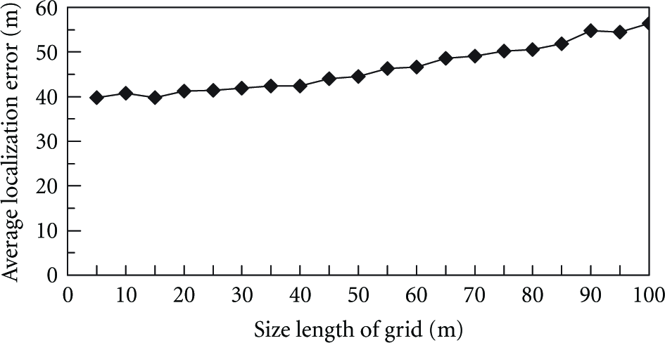
Average localization errors of MAP algorithm under different grid sizes.

5.3. Localization Error

Figure 2 shows a localization result of MAP algorithm and LST algorithm. Both algorithms have the same inputs: σ is set to 5, the number of anchors is set to 20, and the number of sensor nodes is set to 100. It can be seen that the estimated location of most sensor nodes computed by MAP algorithm are closer to their actual locations. Accordingly, MAP algorithm has a smaller average localization error than LST algorithm.

Figure 2

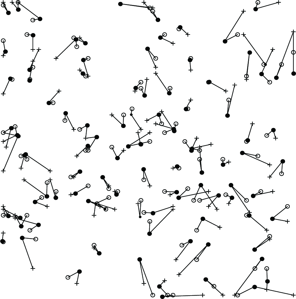
A localization result of MAP algorithm and LST algorithm. In the figure, the solid points represent the actual locations of sensor nodes, the hollow points represent the estimated locations of sensor nodes computed by MAP algorithm, and the cross points represent the estimated locations of sensor nodes computed by LST algorithm.

Next, we test how the localization error is impacted by the number of anchors. In the simulation, σ is set to 5, the number of sensor nodes is set to 100, and the number of anchors varies from 5 to 25. It can be seen from Figure 3 that with the number of anchors increasing, the average localization errors of both algorithms are reduced. But MAP algorithm can achieve a smaller average localization error, which is reduced by nearly 34.8% compared with the least-squares trilateration.

Figure 3

Average localization errors of MAP algorithm and LST algorithm under different numbers of anchors.

Then, we test how the location error is impacted by the layout of anchor nodes. In the simulation, σ is set to 5, the number of sensor node is set to 100, the number of anchors varies among 4, 9, 16, 25, 36, and 49, and anchors are placed by the random layout and the grid layout, respectively. Figure 4 shows the average location errors of MAP algorithm under these two layouts. The average location error under the grid layout is nearly 87.8% of that under the random layout. Therefore, anchor nodes should be placed by the grid layout in practice.

Figure 4

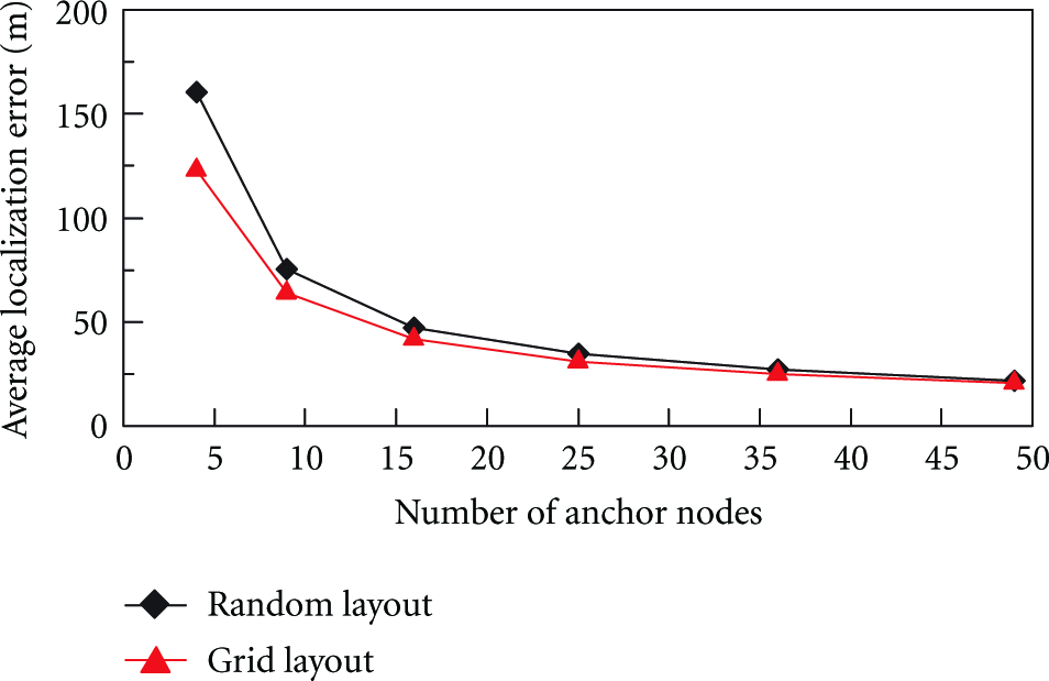
Average localization errors of MAP algorithm under the random layout and the grid layout of anchor nodes.

The ranging error is a primary cause of the localization error, which depends on σ: the larger σ is, the larger the ranging error is. In the simulation, the number of anchors is set to 20, the number of sensor nodes is set to 100, and σ varies from 2 to 14. Figure 5 shows the average localization errors of MAP algorithm and LST algorithm. It can be seen that the average localization errors of both algorithms are approximately proportional to σ.

Figure 5

Average localization errors of MAP algorithm and LST algorithm under different values of σ.

5.4. Fault Tolerance

In MAP algorithm, the location of each sensor node is determined by all its neighbor anchors. If only a small number of anchors are faulty, the estimated location of each sensor node cannot have a big change. In the simulation, σ is set to 5, the number of anchors is set to 20, the number of sensor nodes is set to 100, and the number of faulty anchors varies from 0 to 10. Figure 6 shows the average location errors of MAP algorithm and LST algorithm. It can be seen that when less than 25% of anchors are faulty, the average localization error of MAP algorithm increase less than 85%.

Figure 6

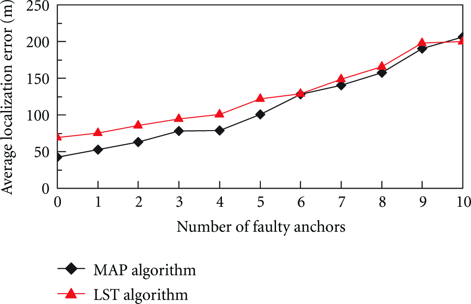
Average localization errors of MAP algorithm and LST algorithm under different numbers of faulty anchors.

5.5. Execution Time

Finally, we analyze the average execution time of MAP algorithm by simulation. In the simulation, the number of sensor nodes is set to 100. Figure 7 shows the average execution times of the two algorithms under different numbers of anchor nodes when the size of grid is 10 m × 10 m. Figure 8 shows the average execution times of the two algorithms under different grid sizes when the number of anchors is 20. It can be seen that the execution times of both algorithms are approximately proportional to the number of anchor nodes and are approximately inversely proportional to the acreage of grid. This result is consistent with the analysis in Section 4. In a general case, MAP algorithm can localize a sensor node in a short time. Since MAP algorithm has a more complicated calculation than LST algorithm, the execution time of MAP algorithm is longer.

Figure 7

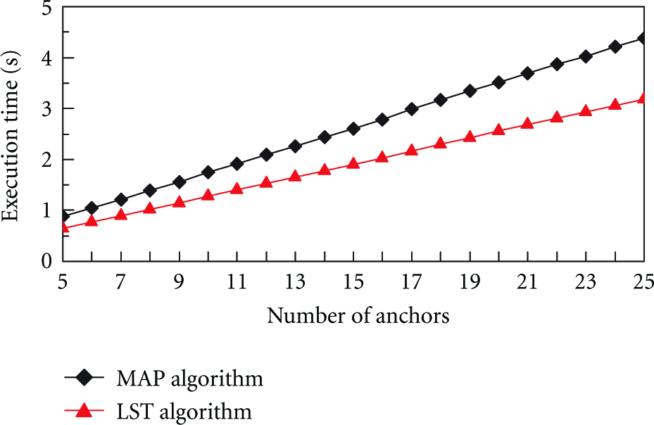
Execution times of MAP algorithm and LST algorithm under different number of anchors.

Figure 8

Execution times of MAP algorithm and LST algorithm under different grid sizes.

6. Conclusion

RSSI ranging-based localization is regarded as a cost-effective solution for sensor node localization. But RSSI ranging technique has a large ranging error, which will bring a large average localization error to the general least-squares trilateration. In this paper, we propose a localization algorithm based on maximum a posteriori probability (MAP). In this algorithm, the point with the maximum probability density in the target region is taken as the estimated location of a sensor node. Extensive simulation results demonstrate the effectiveness of MAP algorithm. This algorithm reduces the average localization error by nearly 34.8% compared with the least-squares trilateration. Even if the number of anchors is small, this algorithm can also achieve a relatively small average localization error. In addition, the execution time of this algorithm is very short.

As a future work, we are currently studying when anchors are absent, how to determine the probability density of the distribution of a sensor node only by the RSSI values of sensor nodes. Moreover, we plan to conduct some practical experiments to confirm the effectiveness of our proposed algorithm.

Footnotes

Acknowledgments

The authors would like to thank the anonymous reviewers for their helpful comments which have significantly improved the quality of the paper. This paper was supported by the National Natural Science Foundation of China (Grant no. 61003272, no. 61033009, no. 61170076, and no. 61103001), the Guangdong Natural Science Foundation (Grant no. 10351806001000000), and the Shenzhen Science and Technology Foundation (Grant no. JC201005280408A and JC2009D3120046A).

References

Akyildiz

I. F.

Vuran

M. C.

Wireless Sensor Networks 2010

John Wiley & Sons

Mao

Fidan

Anderson

B. D. O.

Wireless sensor network localization techniques

Computer Networks 2007 51 10 2529 2553

2-s2.0-34247885928

10.1016/j.comnet.2006.11.018

You

Han

Lieckfeldt

Salzmann

Timmermann

Virtual position based geographic routing for wireless sensor networks

Computer Communications 2010 33 11 1255 1265

2-s2.0-77955273252

10.1016/j.comcom.2009.12.007

Wang

Ghosh

R. K.

Das

S. K.

A survey on sensor localization

Journal of Control Theory and Applications 2010 8 1 2 11

2-s2.0-73549086774

10.1007/s11768-010-9187-7

Zanca

Zorzi

Zanella

Zorzi

Experimental comparison of RSSI-based localization algorithms for indoor wireless sensor networks

Proceedings of the 3rd Workshop on Real-World Wireless Sensor Networks (REALWSN '08)

April 2008

1 5

2-s2.0-62949204512

10.1145/1435473.1435475

Priyantha

N. B.

Chakraborty

Balakrishnan

Cricket location-support system

Proceedings of the 6th Annual International Conference on Mobile Computing and Networking (MOBICOM '00)

August 2000

32 43

2-s2.0-0034539094

Bulusu

Heidemann

Estrin

GPS-less low-cost outdoor localization for very small devices

IEEE Personal Communications 2000 7 5 28 34

2-s2.0-0034291601

10.1109/98.878533

Niculescu

Nath

DV based positioning in Ad Hoc networks

Telecommunication Systems 2003 22 1–4 267 280

2-s2.0-0038703640

10.1023/A:1023403323460

Niculescu

Nath

Ad hoc positioning system (APS) using AOA

Proceedings of the 22nd Annual Joint Conference on the IEEE Computer and Communications Societies (InfoCom '03)

April 2003

1734 1743

2-s2.0-0041973656

10.

Kumar

Kapoor

Range free localization schemes for wireless sensor networks

Proceedings of the 10th WSEAS International Conference on Software Engineering

2011

101 106

11.

Liu

Rendered path: range-free localization in anisotropic sensor networks with holes

IEEE/ACM Transactions on Networking 2010 18 1 320 332

2-s2.0-77249115764

10.1109/TNET.2009.2024940

12.

Lederer

Wang

Gao

Connectivity-based localization of large-scale sensor networks with complex shape

ACM Transactions on Sensor Networks 2009 5 4, article 31

2-s2.0-73349112188

10.1145/1614379.1614383

13.

Doherty

Pister

K. S. J.

El Ghaoui

Convex position estimation in wireless sensor networks

Proceedings of the 20th Annual Joint Conference of the IEEE Computer and Communications Societies (InfoCom '01)

April 2001

1655 1663

2-s2.0-0035013232

14.

Shang

Ruml

Zhang

Fromherz

Localization from connectivity in sensor networks

IEEE Transactions on Parallel and Distributed Systems 2004 15 11 961 974

2-s2.0-8744271199

10.1109/TPDS.2004.67

15.

Kwon

Mechitov

Sundresh

Kim

Agha

Resilient localization for sensor networks in outdoor environments

Proceedings of the 25th IEEE International Conference on Distributed Computing Systems (ICDCS '05)

June 2005

643 652

2-s2.0-27944480938

16.

Khan

U. A.

Kar

Moura

J. M. F.

Distributed sensor localization in random environments using minimal number of anchor nodes

IEEE Transactions on Signal Processing 2009 57 5 2000 2016

2-s2.0-65649092098

10.1109/TSP.2009.2014812

17.

Ding

Krislock

Qian

Wolkowicz

Sensor network localization, Euclidean distance matrix completions, and graph realization

Proceedings of the 1st ACM International Workshop on Mobile Entity Localization and Tracking in GPS-Less Environments (MELT '08)

2008

129 134

18.

Zhu

Gortler

S. J.

Thurston

Sensor network localization using sensor perturbation

ACM Transactions on Sensor Networks 2011 7 4 36

19.

Yedavalli

Krishnamachari

Ravulat

Srinivasan

Ecolocation: a sequence based technique for RF localization in wireless sensor networks

Proceedings of the 4th International Symposium on Information Processing in Sensor Networks (IPSN '05)

April 2005

285 292

2-s2.0-33744918523

10.1109/IPSN.2005.1440937