Sage Journals: Discover world-class research

Abstract

Area coverage is one of the key issues for wireless sensor networks. It aims at selecting a minimum number of sensor nodes to cover the whole sensing region and maximizing the lifetime of the network. In this paper, we discuss the energy-efficient area coverage problem considering boundary effects in a new perspective, that is, transforming the area coverage problem to the target coverage problem and then achieving full area coverage by covering all the targets in the converted target coverage problem. Thus, the coverage of every point in the sensing region is transformed to the coverage of a fraction of targets. Two schemes for the converted target coverage are proposed, which can generate cover sets covering all the targets. The network constructed by sensor nodes in the cover set is proved to be connected. Compared with the previous algorithms, simulation results show that the proposed algorithm can prolong the lifetime of the network.

1. Introduction

With development of wireless communication technology and microelectromechanical system (MEMS) technology, the cost, power, and volume of sensors decrease, while functions increase. Sensors can sense data or events in sensing regions, handle them, communicate with other sensors, and finally transmit the processed data to the base station.

In recent years, wireless sensor networks (WSNs) have been used extensively in many fields, such as monitoring the living environments and behaviors of wild animals [1], detecting the temperature and pressure of craters and earthquakes [2], military supervising, tracking targets, health cares, and vehicular applications [3, 4]. In a WSN, the batteries of sensors are limited and it is not feasible to recharge for large numbers of sensors in many applications. In such an energy-constrained WSN, if sensors are all in the working state simultaneously, excess energy would be wasted and the collected data would be highly correlated and redundant. Therefore, it is critical to make an effective schedule to let one subset of sensors in the working state and the remaining in the sleeping state such that the sensing region can be covered in a long time without recharging. Coverage problems in WSNs have been widely studied [5–8] and can be classified into the following three types [9].

Area coverage [10–13] is to cover a sensing region. Sensors are randomly or deliberately deployed to cover every point in the region.

Target coverage [14–16] is to cover a target set. Sensors and targets are deployed in a region and sensors can cover all the targets in the target set.

Barrier coverage [17, 18] is to cover a long belt region. A belt region is covered if an intruder is detected when crossing the region along any path.

These three kinds of coverage are shown in Figure 1.

Figure 1

Three kinds of coverage.

In this paper, we mainly discuss the area coverage problem, which is similar to the art gallery problem [19] in computational geometry. In the art gallery problem, cameras are placed such that every point in the art gallery is monitored by at least one camera. In area coverage, sensors are deployed and scheduled such that every point in the sensing region can be covered by at least one sensor. Full coverage and connectivity are two important requirements for WSNs. The environment can not be monitored in an accurate way without full coverage and sensor nodes can not communicate with each other to process the sensed data and transmit them to the base station without connectivity.

In recent years, many approaches have been proposed for area coverage problems and target coverage problems, respectively. However, few results integrate them together. In this paper, we study area coverage problems by applying an approach that can solve target coverage problems effectively.

The main contributions of the paper are as follows. (1)

We design an energy-efficient approach for area coverage problems from a new perspective, that is, solving the area coverage problems by transforming the area coverage problem to the target coverage problem.

(2)

We propose two dynamic schemes for the converted target coverage problems to generate cover sets and prove that these cover sets can cover the sensing region completely. Compared with the previous works, our approach can prolong the lifetime of the network significantly by simulations. The two schemes can also be used in the general target coverage problems.

(3)

We prove that as long as the sensing region is completely covered, the network is connected when the communication radius of every sensor node is no smaller than twice of its sensing radius.

The rest of the paper is organized as follows. Section 2 gives the existing results about area coverage, target coverage and connectivity. Section 3 gives the problem statement, some definitions, and assumptions. Section 4 gives the proposed algorithm and two schemes to generate cover sets. In Section 5, we discuss the performance of the algorithm. In Section 6, we show the superiority of our algorithm by simulations. Finally, Section 7 concludes the paper.

2. Related Works

We mainly consider the problem of transforming area coverage to target coverage to maintain coverage and connectivity simultaneously. We now give some related works about area coverage, target coverage, and connectivity in this section.

2.1. Area Coverage

Area coverage is to cover or monitor a region such that every point in it can be covered by at least one sensor node.

In [11], Zalyubovskiy et al. proposed an energy-efficient algorithm for area coverage problems. The locations of sensor nodes are determined and their sensing ranges and communication ranges are adjustable. The algorithm adjusts the sensing radii of sensor nodes and arranges them optimally. In addition, the authors gave two types of coverage models. In the first model, the centers of three neighboring disks with the same sensing radius are connected to be an equilateral triangle. In the second model, the centers of four neighboring disks with the same sensing radius are connected to be a square.

In [12], Misra et al. proposed a coverage algorithm based on Euclidean distance. It requires a cluster head node with high-power, high-computation, and communication capacity for each local region. These cluster heads communicate with common sensor nodes in the same local region, deal with their locations, and generate cover sets independently. A new one will be activated after a cover set finishes its work.

In [13], Kasbekar et al. proposed a polynomial time and distributed k-coverage algorithm to maximize the network lifetime. The algorithm does not require the knowledge of locations of sensor nodes and directional information, but only needs to know the distance between any two communication neighbors and their sensing radii. The algorithm includes two phases, initialization phase and activation phase. In the initialization phase, every node u knows local information including the intersection point set $P_{u}$ covered by it, the set of sensor nodes $T_{u}$ , and $P_{u} ⋂ P_{v}$ , where $T_{u}$ contains sensor nodes covering intersection points in $P_{u}$ and $P_{v}$ is the intersection point set covered by sensor node $v (v \in T_{u})$ . In addition, it also has global information including the number of sensor nodes deployed and the maximum of the initial energy of all sensor nodes. In the activation phase, every sensor node is assigned a weight, called activation preference. Sensor node u competes with the sensor nodes in $T_{u}$ for being an active node according to their activation preferences. A contending sensor node u activates itself once it detects that it has a lower activation preference than all the contending sensor nodes in $T_{u}$ . Once a sensor node u detects that all the intersection points in its sensing range in $P_{u}$ are k-covered by the already active sensor nodes in $T_{u}$ , it enters the sleeping state. The algorithm guarantees that the sensing region is covered completely, whereas it does not consider the tradeoff between energy and coverage. If there is only one intersection point uncovered in the sensing range of a sensor node, the node must be activated, which is against saving energy.

2.2. Target Coverage

Target coverage is to cover a target set such that all the targets in it can be covered by at least one sensor node.

In [14], Cardei et al. proposed a centralized solution based on linear programming (LP) to generate nondisjoint cover sets for the target coverage problem. It takes a high complexity of $O (m^{3} n^{3})$ , where m is the number of cover sets and n is the number of sensor nodes. The authors also proposed a greedy algorithm, with a lower complexity of $O (d k^{2} n)$ , where d is the minimum number of sensor nodes that cover all the targets and k is the number of targets.

In [15], Zorbas et al. proposed an effective coverage algorithm (CCF) for target coverage. CCF divides all the sensor nodes into cover sets, each of which can cover all the targets. These cover sets are disjoint or nondisjoint. The algorithm assigns a weight for each sensor node u, which combines both its monitoring capacity and remaining energy. The authors gave a static-CCF scheme and a dynamic-CCF scheme to produce cover sets, respectively. During the construction of cover sets, the node with a higher weight is preferred to be selected. The static-CCF assigns a weight for every node to describe its relation with Critical Targets. The weight is computed only once at the beginning of the algorithm, and it remains constant until the termination of the algorithm. On the other hand, in the dynamic-CCF scheme, the weight varies dynamically with the set of critical targets during the process of the scheme.

In [16], Shih et al. mainly considered the connected target coverage (CTC) problem in wireless heterogeneous sensor networks with multiple sensing units. The problem can be reduced to a connected set cover problem and further formulated as an integer linear programming (ILP) problem. However, the ILP problem is NP-complete. Therefore, two distributed heuristic schemes, REFS (Remaining Energy First Scheme) and EEFS (Energy Efficiency First Scheme), were proposed. In REFS, each sensor node determines whether it should activate itself such that all targets can be covered and the sensed data can be delivered to the sink, according to its remaining energy and the decisions of its neighbors. The advantages of REFS are its simplicity and reduced communication overhead. To utilize energy of sensor nodes efficiently, EEFS was proposed. In EEFS, the sensor node considers its contribution to coverage and connectivity to make a better decision.

3. Definitions of the Problem

We give some assumptions and definitions before describing the problem.

Assumption 1.

All the sensor nodes are randomly deployed in a sensing region 𝒜, and 𝒜 can be completely covered. If 𝒜 is very large, we divide it into several smaller subregions by following a divide-and-conquer approach [12]. Each of them executes the algorithm independently.

Assumption 2.

All the sensor nodes are static and location-aware. Every node has a unique ID to identify itself, and their locations can be obtained via some localization techniques [20].

Assumption 3.

All sensor nodes have the same sensing radius and the same communication radius; that is, all the sensor nodes are homogeneous.

Assumption 4.

The sensing range of a sensor node u is a disk of radius r, centered at the location of u. A sensor node v located within the sensing range of u is denoted by $v \in SN (u)$ . If the distance between point p in the sensing region and u is less than r, that is, $dist (p, u) < r$ , p is covered by u. The communication range of a sensor node u is a disk of radius R, centered at the location of u. A sensor node w located within the communication range of u is denoted by $w \in CN (u)$ . If the distance between u and w is less than R, that is, $dist (w, u) < R$ , they can communicate with each other.

Assumption 5.

To guarantee the connectivity of the network, the communication radius R of each node must be no smaller than twice of its sensing radius r, which will be proved in Theorem 8. If the network is not connected, the sensed data can not be delivered to the base station and the paper will lose real significance.

Definition 1.

Given a convex region 𝒜, if every point $p \in 𝒜$ is covered by at least one sensor node, then 𝒜 is covered. This kind of coverage is called area coverage.

Definition 2.

Given a target set T, if each target $t \in T$ is covered by at least one sensor node, then T is covered. This kind of coverage is called target coverage.

Definition 3.

The set composed of sensor nodes in the working state and satisfying the requirement of area coverage or target coverage is called cover set. If some sensor nodes belong to different cover sets, these cover sets are called nondisjoint cover sets. If each sensor node belongs to only one cover set, these cover sets are disjoint cover sets. The size of cover sets is an important measurement of the performance of one scheduling algorithm. The smaller a cover set is, the less the energy consumption is.

Definition 4.

Network lifetime is the time interval from the activation of the network until the first time at which a coverage hole appears, or from the point that the network starts operation until the set consisting of all the sensor nodes with nonzero remaining energy is not a cover set any more.

According to the assumptions and definitions above, we can describe the problem as follows.

Given a convex region 𝒜, transform the area coverage to the target coverage and find efficient strategies for target coverage to generate as many cover sets as possible such that nodes in each cover set can cover all the targets in the converted target coverage problem.

4. Algorithm Description

In this section, we propose an algorithm for the area coverage problem with boundary effects (Pseudocode 1). The algorithm includes two phases, transformation phase and cover set generation phase. The former considers how to transform the area coverage problem to the target coverage problem. In this phase, a large sensing region is divided into several smaller subregions, and in each of which, there are some parameters and information of intersection points among disks of sensor nodes or between disks of sensor nodes and boundaries, which can be used as the input of the second phase. These intersection points are the targets in the second phase. In the second phase, we propose two-centralized schemes for the converted target coverage problem obtained from the first phase. Each sub-region executes them independently. The two schemes generate cover sets that can cover all the targets obtained from the first phase. In both of the two schemes, every sensor node is assigned a weight. When selecting a new sensor node for a cover set, the node with a larger weight is preferred. The process operates until the target set is empty. Then a new cover set is generated. Obviously, the two schemes can also be used in the general target coverage problems.

Pseudocode 1: Area coverage algorithm.

Input $S \neq \emptyset$ , $T \neq \emptyset$ , $w > 0$ , $C_{\max} = \emptyset$ , $C_{cur} = \emptyset$ , $C = \emptyset$ ,

$S_{remain} = S$ , $T_{remain} = \emptyset$ , $max_sets = 0$ .

Output $C_{\max}$

Initially, $L_{s_{j}} = w$ , $N_{i} = \emptyset$ , $Q_{j} = \emptyset$ .

/*The following is the transformation phase*/

for all $u \in S$ do

for all $v \in S$ do

if $dist (u, v) < 2 r$ then

$T = T \cup {(u, v, 1), (u, v, 2)}$

end if

end for

for all $u \in S$ do

for all $l \in 𝒜$ do /* for all boundaries of 𝒜*/

if $dist (u, l) < r$ then

$T = T \cup {(u, l, 1), (u, l, 2)}$

end if

end for

for all $t_{i} \in T$ do

for all $s_{j} \in S$ do

if $dist (t_{i}, s_{j}) < r$ then

$N_{i} = N_{i} \cup {s_{j}}$

$Q_{j} = Q_{j} \cup {t_{i}}$

end if

end for

$x = \min {| N_{i} |, t_{i} \in T}$

$max_sets = x \times w$

/* The transformation phase ends*/

/*The following is the cover set generation phase*/

while $S_{remain} \neq \emptyset$ and $| C_{\max} | < max_sets$ do

Algorithm 1 or Algorithm 2

$C_{\max} = C_{\max} \cup {C}$

end while

/* The cover set generation phase ends*/

return $C_{\max}$

4.1. Transformation Phase

If sensor nodes are randomly deployed in a large convex sensing region 𝒜, 𝒜 can be divided into several subregions, that is, $𝒜 = 𝒜_{1} ⋃_{} ‍ 𝒜_{2} ⋃_{} ‍, \dots, ⋃_{} ‍ 𝒜_{k}$ , where k is the number of subregions. Each sub-region has at least one virtual boundary. Given two sensor nodes $w, z \in S$ , where S is the set of sensor nodes deployed in the sensing region 𝒜, if their sensing disks intersect (not tangent), that is, $0 < d (w, z) < 2 r$ , we say w intersects with z. If the distance between a sensor node and one boundary of the region is less than r, we say the node intersects with the boundary. In Figure 2, suppose the sensing region is a rectangle ABCD, we divide it into four smaller subregions and the dotted lines $l_{1}$ and $l_{2}$ are the virtual boundaries: $dist (l_{1}^{'}, l_{1}) = dist (l_{1}^{′′}, l_{1}) = dist (l_{2}^{′′}, l_{2}) = dist (l_{2}^{'}, l_{2}) = 2 r$ . When nodes (such as u and v) are located between $l_{1}^{'}$ and $l_{1}^{′′}$ or between $l_{2}^{'}$ and $l_{2}^{′′}$ , the intersection points ( $t_{1}$ and $t_{2}$ ) among disks of sensor nodes in different subregions can not be ignored. We let the intersection points among disks of sensor nodes or between disks of sensor nodes and boundaries (not including virtual boundaries) be the targets forming a target set used in the second phase, denoted by T, $T = {t_{0}, t_{1}, \dots, t_{m}}$ ; $t_{j}$ is the target and m is the number of targets in T. Each target in T is assigned an ID. If the number of targets in T at the same place exceeds one, we regard them as a single target and assign only one ID for them.

Figure 2

The dotted lines are the virtual boundaries between two subregions.

Theorem 5.

Given a set of sensor nodes $C \subset S$ , if C covers all targets in T, then C is a cover set that can cover the sensing region 𝒜 completely.

Proof.

By contradiction, assume that all targets in T are covered, but there is a small region not covered, denoted by D and p is a point in D. D can be one of the following two cases.

Case 1.

Point p lies in a region D whose boundary is only composed of exterior arcs of a collection of sensing disks (see Figure 3). Since the sensing disks themselves are outside the sensing range of sensor nodes (see Assumption 4 in Section 3), the entire boundary of D, including the intersection points of sensing disks, is not covered. This contradicts the assertion that all targets are covered.

Figure 3

D is bounded by exterior arcs of a collection of sensing disks.

Case 2.

Point p lies in a region D bounded by exterior arcs of a collection of sensing disks and boundaries. As shown in Figure 4, D is in a region bounded by exterior arcs of nodes u, v, x, and the lower boundary. Similarly to Case 1, the entire boundary of D, including the intersection points of nodes u, v, and x and intersection points between nodes v, x, and the lower boundary, is not covered. This contradicts the assertion that all targets are covered.

Figure 4

D is bounded by exterior arcs of a collection of sensing disks and the lower boundary.

In summary, C that covers all the intersection points among disks of sensor nodes or between disks of sensor nodes and boundaries (not including virtual boundaries) can also cover the whole sensing region. Thus, the theorem is true and we can transform the area coverage problem to the target coverage problem.

4.2. Cover Set Generation Phase

In this phase, we propose two dynamic cover set generation schemes (Algorithms 1 and 2) for the converted target coverage problem. Both of them can generate cover sets to cover all the targets in T.

Algorithm 1

Input The target set T.

Output A cover set C

if $T_{remain} \neq \emptyset$ then

$selected = none$

for all $s_{j} \in S_{cur}$ do

$weight (s_{j}) = | Q_{j} |$

end for

$weight (u) = \max {weight (s_{j}), s_{j} \in S_{cur}}$

/*If there is more than one sensor node that

has the largest weight in $S_{cur}$ , the one with

more energy is selected.*/

$selected = u$

if $selected = none$ then

return $C_{\max}$

end if

while $selected \neq none$ and $T_{remain} \neq \emptyset$ do

$L_{selected} = L_{selected} - 1$

$weight (selected) = 0$

if $L_{selected} < 1$ then

$S_{remain} = S_{remain} - {selected}$

end if

$S_{cur} = S_{cur} - {selected}$

$T_{covered} = T_{covered} + Q_{selected}$

$T_{remain} = T_{remain} - Q_{selected}$

$C_{cur} = C_{cur} + {selected}$

for all $t_{i} \in Q_{selected}$ do

for all $s_{j} \in N_{i}$ do

$weight (s_{j}) = weight (s_{j}) - 1$

if $weight (s_{j}) = 0$ then

$S_{cur} = S_{cur} - {s_{j}}$

end if

end for

for all $t_{i} \in Q_{selected}$ do

$S_{avail} = N_{i} ⋃_{} ‍ C N (selected) ⋂_{} ‍ S_{cur}$

end for

if $S_{avail} = \emptyset$ then

$selected = none$

else

$weight (x) = \max {weight (s_{j}), s_{j} \in S_{avail}}$

/*If there is more than one sensor node that

has the largest weight in $S_{avail}$ , the one with

more energy is selected.*/

$selected = x$

end if

end while

output $C = C_{cur}$

end if

Algorithm 2

Input The target set T.

Output A cover set C

if $T_{remain} \neq \emptyset$ then

$selected = none$

for all $s_{j} \in S_{cur}$ do

$W (s_{j}) = | Q_{j} |$

$weight (s_{j}) = a \times (W (s_{j}) / | Q_{j} |) + b \times (L_{s_{j}} / w)$

end for

$weight (u) = \max {weight (s_{j}), s_{j} \in S_{cur}}$

$selected = u$

if $selected = none$ then

return $C_{\max}$

end if

while $selected \neq none$ and $T_{remain} \neq \emptyset$ do

$L_{selected} = L_{selected} - 1$

$W (selected) = 0$

$weight (selected) = 0$

if $L_{selected} < 1$ then

$S_{remain} = S_{remain} - {selected}$

end if

$S_{cur} = S_{cur} - {selected}$

$T_{covered} = T_{covered} + Q_{selected}$

$T_{remain} = T_{remain} - Q_{selected}$

$C_{cur} = C_{cur} + {selected}$

for all $t_{i} \in Q_{selected}$ do

for all $s_{j} \in N_{i}$ do

$W (s_{j}) = W (s_{j}) - 1$

if $W (s_{j}) = 0$ then

$S_{cur} = S_{cur} - {s_{j}}$

$weight (s_{j}) = 0$

end if

end for

for all $t_{i} \in Q_{selected}$ do

$S_{avail} = N_{i} ⋃_{} ‍ C N (selected) ⋂_{} ‍ S_{cur}$

end for

for all $s_{j} \in S_{avail}$ do

$weight (s_{j}) = a \times (W (s_{j}) / | Q_{j} |) + b \times (L_{s_{j}} / w)$

end for

if $S_{avail} = \emptyset$ then

$selected = none$

else

$weight (x) = \max {weight (s_{j}), s_{j} \in S_{avail}}$

$selected = x$

end if

end while

output $C = C_{cur}$

end if

Before executing the two schemes, the following parameters need to be stated.

$N_{i}$ is the set of sensor nodes covering the target $t_{i}$ ; that is, $N_{i} = {s_{j} | dist (s_{j}, t_{i}) < r, j = 1, \dots, n$ , n is the number of sensor nodes}, where $i = 1, \dots, m$ , and m is the number of targets. $| N_{i} |$ is the number of sensor nodes covering target $t_{i}$ .

$Q_{j}$ is the set of targets covered by the sensor node $s_{j}$ , that is, $Q_{j} = {t_{i} | dist (s_{j}, t_{i}) < r, i = 1, \dots, m}$ , where $j = 1, \dots, n$ , and n is the number of sensor nodes.

$C_{cur}$ is a set of sensor nodes that have already been selected into the cover set currently. Initially, $C_{cur} = \emptyset$ .

C is the cover set produced by the two schemes, and $C_{cur} \subset C$ .

$C_{\max}$ is the set of all cover sets. $| C_{\max} |$ is the number of cover sets.

S is the set of sensor nodes deployed.

$S_{remain}$ is the set of sensor nodes with nonzero energy. Initially, $S_{remain} = S$ .

$S_{cur}$ is the set of sensor nodes currently remaining with nonzero energy except the sensor nodes that have been added into the current cover set $C_{cur}$ .

$S_{avail}$ is the set of candidate sensor nodes that have not been added but could be added into the current cover set $C_{cur}$ . Initially, $S_{avail} = \emptyset$ .

T is the set of intersection points obtained in the transformation phase.

$T_{remain}$ is the target set uncovered. Initially, $T_{remain} = T$ .

$T_{covered}$ is the target set including the targets already covered by sensor nodes in the current cover set $C_{cur}$ .

w is the number of cover sets that each sensor can participate in initially.

$L_{s_{j}}$ is the remaining number of cover sets that the sensor node $s_{j}$ can participate in currently. Initially, $L_{s_{j}} = w$ .

$W (s_{j})$ is the number of targets lying in the sensing range of $s_{j}$ but uncovered by other nodes that have been selected for $C_{cur}$ .

$weight (s_{j})$ is the weight of the node $s_{j}$ assigned by the two cover set generation schemes.

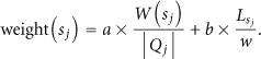
Initially, Algorithm 1 assigns a weight for every sensor node $s_{j}$ , that is, $weight (s_{j}) = | Q_{j} |$ , which means the number of targets lying inside the sensing range of $s_{j}$ but uncovered by other nodes that have been selected for $C_{cur}$ . Afterwards, an initial sensor node that has the largest weight is selected from $S_{cur}$ . If there is more than one sensor node that has the largest weight in $S_{cur}$ , the one with more energy is selected. If there is no sensor node in $S_{cur}$ , Algorithm 1 ends. After selecting a new node, denoted by $selected$ , Algorithm 1 removes it from $S_{cur}$ , adds it into $C_{cur}$ , removes the targets covered by it from $T_{remain}$ , and puts them into $T_{covered}$ . But the targets that have ever been added into $T_{covered}$ will not be added again. For each target $t_{i}$ in $Q_{selected}$ , the weight of each node $s_{j}$ in $N_{i}$ decreases by 1, that is, $weight (s_{j}) = weight (s_{j}) - 1$ , which is to bring down the possibility of being selected. If the weight of a sensor node is 0, which implies the targets covered by it have already been covered by other sensor nodes in $C_{cur}$ , it will be removed from $S_{cur}$ . Afterwards, the sensor nodes with nonzero weights in $N_{i}$ and $CN (selected)$ are put into the set $S_{avail}$ , and the nodes that have ever been added into $S_{avail}$ will not be added again. Then the sensor node in $S_{avail}$ with the largest weight is selected for $C_{cur}$ ; that is, the node that can cover the largest number of targets uncovered by other nodes in $C_{cur}$ until now is selected. Loop until all the targets are covered and $T_{remain}$ is empty or $S_{avail}$ is empty. Then $C_{cur}$ becomes a cover set C.

Initially, Algorithm 2 assigns a weight for every sensor node $s_{j}$ with $weight (s_{j}) = a \times (W (s_{j}) / | Q_{j} |) + b \times (L_{s_{j}} / w)$ , where $a + b = 1$ . a and b are parameters used to decide the percentage of residual energy and the percentage of the number of uncovered targets. a and b are initialized at the beginning of the application and do not change during the application lifetime. $W (s_{j}) / | Q_{j} |$ is used to describe the current coverage contribution of sensor node $s_{j}$ , where $W (s_{j})$ is the number of targets lying in the sensing range of $s_{j}$ but uncovered by other nodes that have been selected for $C_{cur}$ . $L_{s_{j}} / w$ can be used to describe the energy available currently. The process of Algorithm 2 is similar to that of Algorithm 1. When selecting a sensor node for a cover set, Algorithm 1 emphasizes on its coverage contribution, that is to say, selecting the one covering as many targets uncovered as possible in T, while Algorithm 2 considers the tradeoff between energy and coverage contribution.

We prove the correctness of the two cover set generation schemes above now.

Theorem 6.

Both of the two schemes can generate at least one cover set, if there exists one in the network.

Proof.

Assume that $C_{1}$ is a cover set. For

\begin{matrix} \forall t_{i} \in T, \exists s_{j} \in C_{1}, s . t . t_{i} \in Q_{j}, \end{matrix}

(1)

where

C_{1} \subseteq S

C_{1} \neq \emptyset

Q_{j} \subseteq T

, and

Q_{j} \neq \emptyset

By contradiction, suppose that $C_{1}$ does exist, that is to say, sensor nodes in S can cover all the targets in T. However, our schemes can not produce a cover set, which means that there does not exist a sensor node $s_{j}$ in $S_{cur}$ such that $s_{j}$ can cover targets in $T_{remian}$ , for

\begin{matrix} \forall t_{i} \in T_{remain}, \neg \exists s_{j} \in S_{cur}, s . t . t_{i} \in Q_{j} . \end{matrix}

(2)

C_{cur}

is a set of nodes that have already been selected into the cover set, and

\begin{matrix} S = C_{cur} \cup S_{cur}, C_{cur} \cap S_{cur} = \emptyset . \end{matrix}

(3)

Remove all the targets covered by nodes in

C_{cur}

from

T_{remain}

. Then, for

\begin{matrix} \forall t_{i} \in T_{remain}, \neg \exists s_{j} \in C_{cur}, s . t . t_{i} \in Q_{_{j}} . \end{matrix}

(4)

From (2), (3), (4), we have

\begin{matrix} \forall t_{i} \in T_{remain}, \neg \exists s_{j} \in S, s . t . t_{i} \in Q_{j} . \end{matrix}

(5)

In addition,

T_{remain} \subseteq T

C_{1} \subseteq S

, thus (5) contradicts (1), and the initial hypothesis proves to be false. Therefore, our schemes can generate at least one cover set to guarantee full coverage of the sensing region.

5. Algorithm Analysis

In the cover set generation phase, we select sensor nodes for cover sets according to the following three criteria. (1)

The sensor node covering a larger number of targets has a higher priority.

(2)

Minimize the probability of covering a target multiply.

(3)

Promote candidates with more remaining energy.

For (1), Algorithm 1 assigns a weight for every sensor node $s_{j}$ , that is, $weight (s_{j}) = | Q_{j} |$ , and selects a sensor node that has the largest weight.

For (2), in Algorithms 1 and 2, as for every target $t_{i}$ in $Q_{j}$ , the weight of every node in $N_{i}$ decreases to reduce the probability of covering a target multiply after selecting a new node $s_{j}$ for a cover set.

For (3), Algorithm 1 selects a sensor node with more energy when there is more than one node that has the largest weight. When considering the tradeoff between the remaining energy of a sensor node and the number of targets covered by it, we propose Algorithm 2, which combines criterion 1 and 3, and assigns a weight for every sensor node $s_{j}$ as follows.

\begin{matrix} weight (s_{j}) = a \times \frac{W (s_{j})}{| Q_{j} |} + b \times \frac{L_{s_{j}}}{w} . \end{matrix}

(6)

Now, we give the algorithm for solving area coverage problems. The pseudocodes are as follows.

The complexity of the algorithms executed in each sub-region is $O (n^{2} m)$ , where n is the number of sensor nodes in the smaller sub-region and m is the number of targets in the sub-region produced in phase one. Since the number of targets and sensor nodes in sub-region is smaller than those in the whole sensing region, our algorithm is effective.

Since there are many sensor nodes in the sensing region, one target may be covered by multiple sensor nodes. Assume that there are x sensor nodes in the smallest set $N_{i}$ . Initially, each sensor node has the energy with the capability of participating in w cover sets. Thus, the algorithm can produce at most $x \times w$ cover sets, which is an upper bound of the number of cover sets produced and is also a theoretical result, that is, $\max_sets = x \times w$ . When there is no sensor node in $S_{remain}$ or the number of cover sets produced is $\max_sets$ , the algorithm ends and returns $C_{\max}$ . Obviously, the cover sets produced by the algorithm are nondisjoint cover sets.

Both of Theorems 5 and 6 above fit the case in one sub-region, and the proof of coverage in the whole region 𝒜 is as follows.

Theorem 7.

The whole large region 𝒜 can be covered when it is divided into multiple subregions and each of them executes the algorithm independently.

Proof.

We divide a large sensing region 𝒜 into several smaller subregions by following a divide-and-conquer approach in order that our algorithm can be widely used in large sensing regions. In the transformation phase, the intersection points among disks of sensor nodes or between disks of sensor nodes and boundaries (not including virtual boundaries) of subregions are calculated as the targets used in the cover set generation phase. Targets in all these subregions constitute the targets in T. In each sub-region, cover set generation schemes work independently on the targets that also include the intersection points between disks of sensor nodes and virtual boundaries. Thus, the number of targets in all these subregions is more than the number of targets in T. From Theorem 6, the cover sets generated can cover all the targets in each sub-region. Thus, all the targets in T can also be covered. From Theorem 5, if all the targets in T can be covered, the whole region can also be covered. Thus, the theorem is right.

According to the theorem, the proposed algorithm can be applied in large networks with thousands or more nodes.

Theorem 8.

The network constructed by sensor nodes in any cover set is connected when the communication radius of any sensor node is no smaller than twice of its sensing radius.

Proof.

By contradiction, if the network is not connected, there exists a pair of sensor nodes with no path between them. Assume that $(u, v)$ is a pair of nearest (Euclidean distance) sensor nodes that are not connected. Given a disk, denoted by x, which lies on the line segment from u to v, $dist (u, x) = r$ (as is shown in Figure 5).

Figure 5

$(u, v)$ is a pair of nearest sensor nodes that are not connected.

Firstly, we prove that there must be other sensor nodes inside the disk of x. We prove it by contradiction. Assume that there are no other nodes inside the disk. In order to contain another sensor node y, the disk x moves a shortest distance ε along $\vec{u v}$ to the node v and is located at $x^{′′}$ . When the disk moves a distance less than ε along $\vec{u v}$ to the node v and is located at $x^{'}$ , there are still no other nodes inside the disk since $dist (x^{'}, y) > r > dist (x^{′′}, y)$ and $dist (u, x^{'}) > r$ . Thus, the point on the disk center $x^{'}$ is not covered by any sensor node, which contradicts the condition that the whole region is covered completely. Therefore, there must be other sensor nodes inside the disk of x. Assume that a sensor node p is inside the disk of x before moving. Since $dist (p, u) < 2 r$ and $2 r \leq R$ , node u and node p are connected. However, u and v are not connected. Thus, p and v are not connected. Otherwise, u and v are connected. In addition, $dist (u, v) > dist (p, v)$ , for $∠ 1 < π / 2 < ∠ 2$ . This contradicts the hypothesis that $(u, v)$ is a pair of nearest sensor nodes that are not connected. Therefore, the theorem is true.

According to Theorem 8, we can ensure the network connectivity. Then the sensed data can be transmitted to the base station.

6. Simulations

We describe the simulation results from three aspects, the size of cover sets, the number of cover sets, and coverage redundancy. The size of cover sets is the number of working sensor nodes in cover sets. The size of cover sets is inversely proportional to the lifetime of the network. The number of cover sets is the number of cover sets theoretically produced by the algorithm and is directly proportional to the lifetime of the network. When the required coverage degree is 1, the case that every point in the sensing region covered by only one sensor node is hardly achieved for full coverage and the case that many small parts of the sensing region are multicovered is called coverage redundancy. Without considering fault tolerance of the network, coverage redundancy must be reduced when designing an algorithm for coverage problems. The smaller the redundancy is, the longer the lifetime of the network is.

Our algorithm includes two phases, transformation phase and cover set generation phase. The second phase works on the targets generated in the first phase. The schemes in the second phase can also be used in the general target coverage problems. To prove the superiority of our schemes for target coverage problems, we firstly compare our schemes with static-CCF [15]. As shown in Figure 6, t and n are the number of targets and the number of sensor nodes in a $50 m \times 50 m$ region, $a = 0.5$ , $b = 0.5$ in Algorithm 2, $α = β = γ = 1 / 3$ in static-CCF, and $w = 5$ . The sensing radius r of every sensor node is 10 m. Figures 6(a) and 6(c) consider the case that the number of targets t is 500. When the number of nodes increases, the density of nodes increases, and it will generate more cover sets to cover all these targets. Thus, the number of cover sets increases while the average size of cover sets decreases. Figures 6(b) and 6(d) describe the case that the number of sensor nodes n is 400. When the number of targets increases, it will need more sensor nodes to cover all these targets. Thus, the number of cover sets decreases while the average size of cover sets increases. When the number of targets is small, the number of nodes covering them is also small. However, in these three schemes, when the number of targets and the number of sensor nodes is large enough, the average size of cover sets almost the same. From Figure 6, we can conclude that our schemes generate more cover sets than static-CCF, which represents our schemes can prolong the network lifetime compared to static-CCF, since our schemes pay more attention to sensor nodes that can cover more targets uncovered. Therefore, our schemes are energy-efficient.

Figure 6

Compare our schemes with static-CCF.

Figure 6 considers target coverage problems. In the following simulations, we consider area coverage problems. If the sensing region is large, we can divide it into several subregions by following a divide-and-conquer approach. Each sub-region executes the algorithm independently. In the following simulations, we mainly consider one sensing region with the size of $50 m \times 50 m$ and the sensing radius r of every sensor node is 10 m. In the following simulations, the number of cover sets produced by our algorithm is almost the same as the number in theory. When different numbers of sensor nodes are deployed, the number of targets generated differs, and so does the number of cover sets.

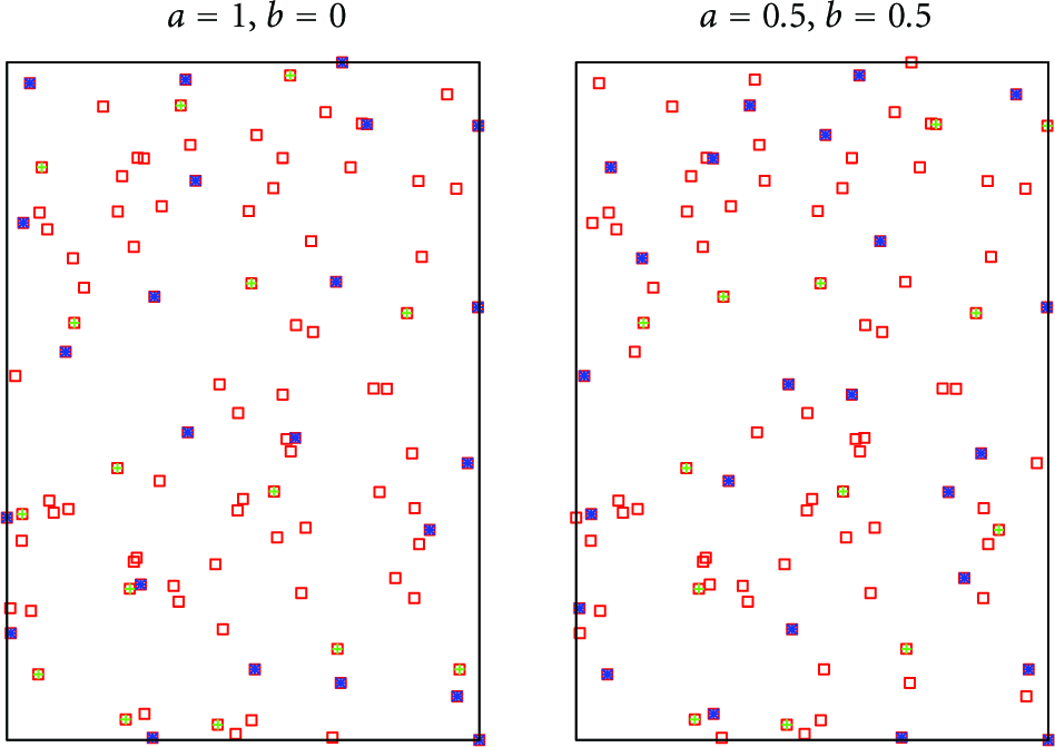
The network topologies under Algorithms 1 and 2 are shown in Figure 7. Only Algorithm 2 considers the values of a and b, and here we only consider the case of $a = 1$ , $b = 0$ and the case of $a = 0.5$ , $b = 0.5$ . In the figure, “ $□$ ” means the sensor nodes deployed, “+” means the working nodes in the cover set generated by Algorithm 1, and “*” means the working nodes in the cover set generated by Algorithm 2. Here, 100 sensor nodes are deployed in a $50 m \times 50 m$ region. Since the first cover set generated by Algorithm 2 remains the same with different values of a and b, we choose the second cover set to describe the network topology.

Figure 7

The network topology.

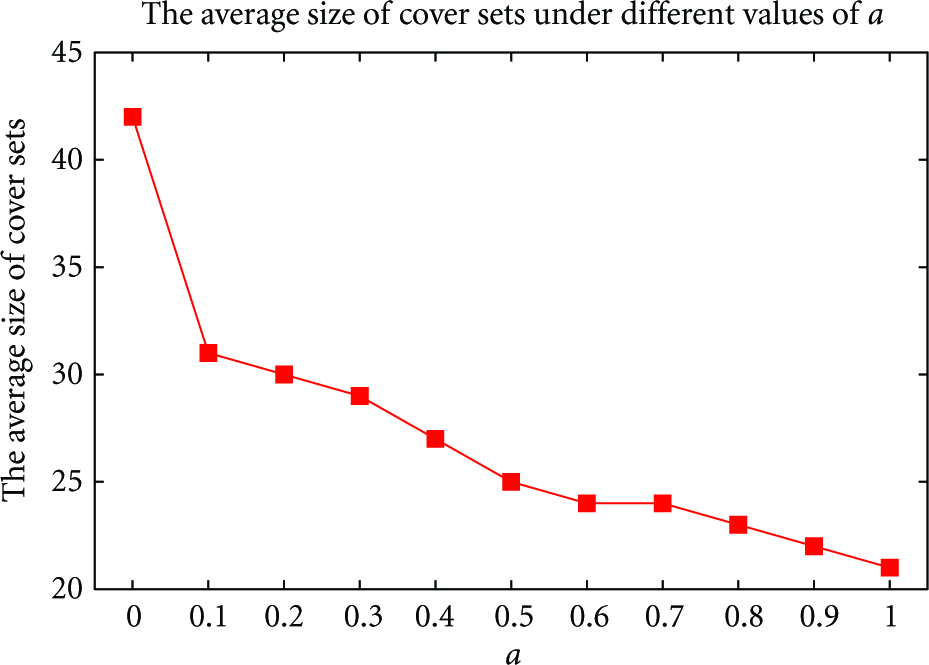
Figure 8 shows the average size of cover sets with $w = 10$ under different values of coefficient a in Algorithm 2. Here, 100 sensor nodes are randomly deployed in the region. When $a = 0$ and $b = 1$ , the remaining energy of sensor nodes is the only factor considered and their coverage contributions are not considered. Thus, the average size of cover sets produced is large. As the value of a increases, the algorithm begins to focus on the coverage contributions of sensor nodes and the average size of cover sets decreases. When $a = 1$ and $b = 0$ , sensor nodes can participate in producing cover sets as long as their remaining energy is enough for covering the region once again.

Figure 8

The average size of cover sets with $w = 10$ under different values of a.

Figure 9 shows the number of cover sets under different numbers of sensor nodes randomly deployed. Here, $a = 0.9$ , $b = 0.1$ , and $w = 10$ . Obviously, the number of cover sets increases with increasing number of sensor nodes. Algorithm 1 can produce more cover sets than Algorithm 2 and CPLC [12]. The reason is that Algorithm 1 selects sensor nodes that can cover a larger number of targets uncovered by other nodes that have been selected for $C_{cur}$ . Algorithm 2 selects sensor nodes that have the largest comprehensive abilities of the remaining energy and the coverage contributions; that is, Algorithm 2 considers both targets remaining uncovered by other nodes in $C_{cur}$ and the residual energy of nodes. When different numbers of sensor nodes are deployed, the number of sensor nodes in the smallest $N_{i}$ differs, and so does the number of cover sets. CPLC firstly selects two nearest sensor nodes, denoted by x and y, and then two furthest neighbors of them in the two communication neighbor sets are selected into the cover set, respectively. The process continues until the two sets are empty. However, some nodes nearby may be all selected. Thus, some redundant sensor nodes are selected into cover sets and the number of cover sets is reduced correspondingly.

Figure 9

The numbers of cover sets under different numbers of sensor nodes deployed.

Figure 10 describes the relation between energy and the number of cover sets produced. Here, $a = 0.9$ , $b = 0.1$ , and $n = 100$ . In our paper, the number of cover sets produced increases linearly with w since the number of cover sets produced is almost the same as the number in theory and the number of cover sets produced in theory is $x \times w$ , where x is a constant since all sensor nodes are static. In CPLC, if we want to guarantee full coverage, the number of cover sets is small.

Figure 10

The relation between energy and the number of cover sets produced.

Figure 11 represents the comparison of the average coverage degrees among CPLC, Algorithms 1 and 2 under different numbers of sensor nodes randomly deployed. When the required coverage degree is 1, many small parts of the sensing region may be multicovered, and the coverage degree of the whole sensing region on average is called the average coverage degree. Obviously, compared to CPLC, the average coverage degree obtained from our proposed schemes is lower; that is, the proportion of the sensing region multicovered is small. Without considering fault tolerance of the network, the lower the average coverage degree is, the less the coverage redundancy is. Here, $w = 5$ , $a = 0.5$ , $b = 0.5$ , and $R = 2 r = 20$ m.

Figure 11

The comparison of the average coverage degrees among CPLC, Algorithms 1 and 2.

Figure 12 represents the comparison of the average size of cover sets under different numbers of sensor nodes deployed. Here, $w = 5$ , $a = 0.5$ , $b = 0.5$ , and $R = 2 r = 20$ m. The average size of cover sets produced by Algorithm 1 remains 20–22 all the time as the number of sensor nodes randomly deployed increases. The average size of cover sets produced by Algorithm 2 increases slowly since it considers the coverage contribution and the remaining energy when selecting sensor nodes. However, when the number of sensor nodes is large enough, the average size of cover sets almost remains 23–25 since the density of sensor nodes is large enough for covering the whole region. The average size of cover sets produced by CPLC is larger than our proposed two schemes. Thus, our algorithm can prolong the network lifetime compared to CPLC. Therefore, our algorithms are energy-efficient.

Figure 12

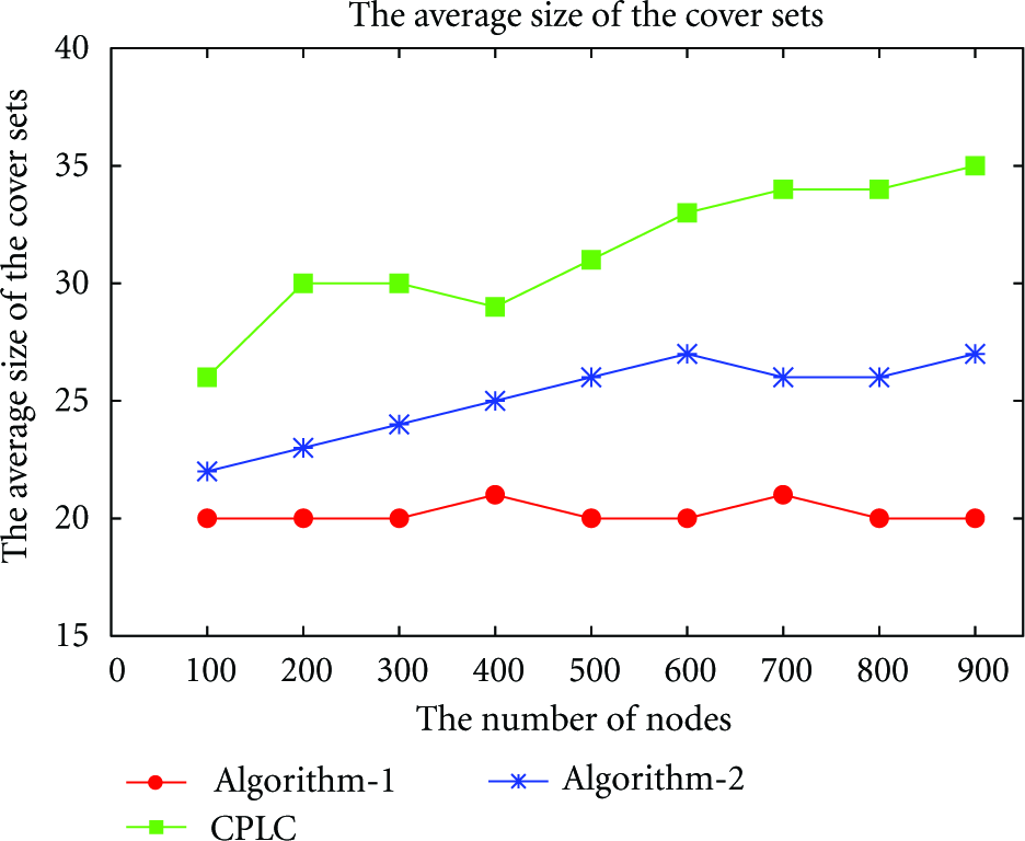
The comparison of the average size of cover sets under different numbers of sensor nodes deployed.

Figure 13 represents the comparison of coverage redundancy under different algorithms. Here, 200 sensor nodes are randomly deployed, $a = 0.5$ , $b = 0.5$ , and $R = 2 r = 20$ m. We compare our algorithm with CPLC [12]. We can obtain the coverage percentage of the sensing region by dividing the region into $1 m \times 1 m$ small squares. In Figure 13, each data column represents the proportion of small squares whose coverage degree is no less than the distributed coverage degree. From Figure 13, we can see that all the squares are 1-covered in these three algorithms. In CPLC, 92.5% of squares are 2-covered, and 19.4% are 4-covered. In Algorithm 1, 70% of squares are 2-covered, and 3.5% are 4-covered. In Algorithm 2, 72% of squares are 2-covered, and 3.9% are 4-covered. We can conclude from Figure 13 that CPLC has the highest coverage redundancy, Algorithm 2 comes second, and Algorithm 1 has the lowest redundancy. Without considering fault tolerance, the lower the redundancy is, the smaller the number of working nodes in the cover set is.

Figure 13

The comparison of coverage redundancy under different algorithms.

7. Conclusion and Future Work

In this paper, we discuss the area coverage problem with boundary effects and propose a new approach that integrates the area coverage with the target coverage and transforms the coverage of all the points in the sensing region to the coverage of a fraction of targets to achieve full area coverage. The algorithm is divided into two phases, transformation phase and cover set generation phase. The first phase is to transform the area coverage problem to the target coverage problem. The second phase gives two cover set generation schemes for the converted target coverage problem. The two schemes can also be used in general target coverage problems. Then, we set the communication radii of sensor nodes no smaller than twice of their sensing radii to guarantee network connectivity. Finally, we prove by simulations that our proposed algorithm is better than other algorithms and that the lifetime of the network is prolonged.

In Section 3, we give some assumptions. Assumption 2 is that every sensor node is static and location-aware. Assumption 3 is that all the sensors are homogeneous. Due to the variety of the real environment, we can relax the two assumptions to be closer to the real environment. For example, we can study the case that the locations of sensor nodes are unknown, and the case that all the sensor nodes are heterogeneous, or both of the two cases.

Footnotes

Acknowledgments

This work was partially supported by the National Natural Science Foundation of China for contract (60373012, 11101243), Natural Science Foundation of Shandong Province for contract (ZR2012FM023, ZR2009GM009), STPU of Shandong Province for contract (J10LG09), and TKP of Shandong Province for contract (2009GG10001014).

References

Mainwaring

Culler

Polastre

Szewczyk

Anderson

Wireless sensor networks for habitat monitoring

Proceedings of the 1st ACM International Workshop on Wireless Sensor Networks and Applications

September 2002

New York, NY, USA

88 97

2-s2.0-0036986465

Allen

G. W.

Lorincz

Johnson

Lees

Welsh

Fidelity and yield in a volcano monitoring sensor network

Proceedings of the 7th symposium on Operating Systems Design and Implementation

2006

Berkeley, Calif, USA

381 396

Akyildiz

I. F.

Sankarasubramaniam

Cayirci

Wireless sensor networks: a survey

Computer Networks 2002 38 4 393 422

2-s2.0-0037086890

10.1016/S1389-1286(01)00302-4

Liu

Energy conservation algorithms for maintaining coverage and connectivity in wireless sensor networks

IET Communications 2010 4 7 786 800

2-s2.0-77956940213

10.1049/iet-com.2009.0129

Meguerdichian

Koushanfar

Potkonjak

Srivastava

M. B.

Coverage problems in wireless ad-hoc sensor networks

Proceedings of the IEEE INFOCOM 2001

April 2001

1380 1387

2-s2.0-0034997317

Huang

C. F.

Tseng

Y. C.

The coverage problem in a wireless sensor network

Proceedings of the 2nd ACM International Workshop on Wireless Sensor Networks and Applications (WSNA'03)

September 2003

115 121

2-s2.0-1542286906

Ghosh

Das

S. K.

Coverage and connectivity issues in wireless sensor networks: a survey

Pervasive and Mobile Computing 2008 4 3 303 334

2-s2.0-43549098529

10.1016/j.pmcj.2008.02.001

Huang

C. F.

Tseng

Y. C.

L. C.

The coverage problem in three-dimensional wireless sensor networks

Proceedings of the IEEE Global Telecommunications Conference (GLOBECOM'04)

December 2004

3182 3186

2-s2.0-18144362070

Cardei

Coverage in wireless sensor networks

Handbook of Sensor Networks: Compact Wireless and Wired Sensing Systems 2005

10.

Carle

Simplot-Ryl

Energy-efficient area monitoring for sensor networks

Computer 2004 37 2 40 46

2-s2.0-10744232231

10.1109/MC.2004.1266294

11.

Zalyubovskiy

Erzin

Astrakov

Choo

Energy-efficient area coverage by with adjustable ranges

Sensors 2009 9 4 2446 2460

10.3390/s90402446

12.

Misra

Kumar

M. P.

Obaidat

M. S.

Connectivity preserving localized coverage algorithm for area monitoring using wireless sensor networks

Computer Communications 2011 34 12 1484 1496

2-s2.0-79959374364

10.1016/j.comcom.2010.03.002

13.

Kasbekar

G. S.

Bejerano

Sarkar

Lifetime and coverage guarantees through distributed coordinate-free sensor activation

IEEE/ACM Transactions on Networking 2011 19 2 470 483

2-s2.0-79955475521

10.1109/TNET.2010.2077648

14.

Cardei

Thai

M. T.

Energy-efficient target coverage in wireless sensor networks

Proceedings of the IEEE INFOCOM 2005

March 2005

1976 1984

2-s2.0-25844504705

15.

Zorbas

Glynos

Kotzanikolaou

Douligeris

Solving coverage problems in wireless sensor networks using cover sets

Ad Hoc Networks 2010 8 4 400 415

2-s2.0-75149197226

10.1016/j.adhoc.2009.10.003

16.

Shih

K. P.

Deng

D. J.

Chang

R. S.

Chen

H. C.

On connected target coverage for wireless heterogeneous sensor networks with multiple sensing units

Sensors 2009 9 7 5173 5200

2-s2.0-70849100697

10.3390/s90705173

17.

Kumar

Lai

T. H.

Arora

Barrier coverage with wireless sensors

Proceedings of the 11th Annual International Conference on Mobile Computing and Networking (MobiCom'05)

September 2005

284 298

2-s2.0-32144431768

10.1145/1080829.1080859

18.

Zhang

Shen

Zheng

Yao

A study on the weak barrier coverage problem in wireless sensor networks

Computer Networks 2011 55 3 711 721

2-s2.0-79951513958

10.1016/j.comnet.2010.10.008

19.

'Rourke

J. O.

Art Gallery Theorems and Algorithms 1987

New York, NY, USA

Oxford University Press

20.

Zha

Sensor positioning in wireless ad-hoc sensor networks using multidimensional scaling

Proceedings of the IEEE INFOCOM 2004

March 2004

2652 2661

2-s2.0-8344227634

Transforming Area Coverage to Target Coverage to Maintain Coverage and Connectivity for Wireless Sensor Networks

Abstract

1. Introduction

2. Related Works

2.1. Area Coverage

2.2. Target Coverage

3. Definitions of the Problem

Assumption 1.

Assumption 2.

Assumption 3.

Assumption 4.

Assumption 5.

Definition 1.

Definition 2.

Definition 3.

Definition 4.

4. Algorithm Description

Pseudocode 1: Area coverage algorithm.

4.1. Transformation Phase

Theorem 5.

Proof.

Case 1.

Case 2.

4.2. Cover Set Generation Phase

Algorithm 1

Algorithm 2

Theorem 6.

Proof.

5. Algorithm Analysis

Theorem 7.

Proof.

Theorem 8.

Proof.

6. Simulations

7. Conclusion and Future Work

Footnotes

Acknowledgments

References