Performance Analysis of Flow-Based Traffic Splitting Strategy on Cluster-Mesh Sensor Networks

Abstract

Performance analysis is crucial for designing predictable and cost-efficient sensor networks. Based on the network calculus theory, we propose a flow-based traffic splitting strategy and its analytical method for worst-case performance analysis on cluster-mesh sensor networks. The traffic splitting strategy can be used to alleviate the problem of uneven network traffic load. The analytical method is able to derive close-form formulas for the worst-case performance in terms of the end-to-end least upper delay bounds for individual flows, the least upper backlog bounds, and power consumptions for individual nodes. Numerical results and simulations are conducted to show benefits of the splitting strategy as well as validate the analytical method. The numerical results show that the splitting strategy enables much better balance on network traffic load and power consumption. Moreover, the simulation results verify that the theoretic bounds are fairly tight.

1. Introduction

With the advances of wireless communications and microelectronics technologies, wireless sensor networks (WSNs) have received more and more attention over the last decades due to their potential in a variety of application domains [1–4], such as environment monitoring, human activity tracking, healthcare, and military assistance, and so forth.

A typical sensor network consists of a larger number of sensor nodes that are capable of sensing the environment and forwarding their observation values to a fusion center (sink) through multihop wireless links. Thus, the traffic pattern in sensor networks is usually in a many-to-one manner. The nodes near the sink may need to forward more data and thus require more energy consumptions and bigger buffers than the nodes far away. Consequently, the distributions of energy and buffer requirements in WSNs are extremely uneven. However, energy supplies and buffers are limited and expensive resources in typical WSNs, since sensor nodes are usually made as tiny devices with limited buffers and equipped with batteries that may not be convenient or economical for replacement. One way to address these challenges is applying traffic splitting strategies which have been adopted by many researchers for load balancing in communication networks [5, 6]. With traffic splitting, a main flow is divided into several subflows and forwarded to the destination through different routing paths. By distributing traffic over the network, the overall network load balance can be improved. It is shown in [7] that the spare capacity can be reduced and thus the overall performance of the system can be improved by splitting traffic across multiple disjoint paths.

One popular application of WSNs is real-time monitoring and tracking, such as logistic chain tracking [4] and healthcare application [8]. In such kind of applications, it is crucial to ensure sensor data delivered to the sink within time constraints so that appropriate actions can be made. In order to design a WSN with predictable delay, backlog, and energy consumptions, formal performance analysis is desired for analyzing a sensor network before its actual deployment. While simulation-based methods can offer high accuracy, it can be very time-consuming and tedious to find the worst-case performance. Each simulation run may take considerable time and evaluates only a single network configuration, traffic pattern, and load point. Hence, formal methods are desired to dimension sensor networks in an analytical way rather than case-by-case simulations. Starting with the initial work by Cruz [9, 10], network calculus has been developed as a useful tool for the performance analysis of networked system [11]. In contrast to queueing theory, network calculus deals with performance bounds, such as worst-case delay and backlog bounds, rather than average values. It has been applied to sensor networks by many researchers recently [12–15].

In this paper, we propose a flow-based traffic splitting strategy and its analytical method for worst-case performance analysis on cluster-mesh sensor networks based on the network calculus theory. We introduce the flow-based traffic splitting strategy, which is useful in balancing not only network load but also power consumption. Aiming to evaluate the worst-case performance in terms of end-to-end least upper delay bound, least upper backlog bound, and power consumption, a splitting model is built for a single-node analysis and an analytical method is proposed for the network analysis. Through an example, we show that the performance analysis method is able to derive closed-form formulas of these bounds. The numerical results indicate that the backlog and power consumption can be balanced by applying the traffic splitting strategy. In addition, simulations are performed to validate the performance bounds of our analytical method. The results show that their tightnesses are satisfactory.

The rest of this paper is organized as follows. Section 2 introduces related work. Section 3 contains preliminaries including the cluster-mesh network topology and power consumption model, and basics of network calculus. Section 4 includes performance analysis of the flow-based traffic splitting strategy. An analysis example is given in Section 5. Numerical results and simulations are presented in Section 6. Finally, conclusions and directions for future work are given in Section 7.

2. Related Work

In general packet switching networks, network calculus provides methods to deterministically reason about timing properties and resource requirements. Based on the powerful abstraction of arrival curve for traffic flows and service curve for network elements, it allows computing the worst-case delay and backlog bounds. Systematic accounts of network calculus can be found in books [11, 16].

Network calculus has been extremely successful for ensuring performance bounds when applied to ATM, Internet, and other networks. It is recently extended and applied for performance analysis and resource dimensioning of WSNs by several researchers. In [12], Schmitt and Roedig firstly applied network calculus to sensor network and proposed a generic framework for performance analysis of WSNs with various traffic patterns. They further extended the general framework to incorporate computational resources besides the communication aspects of WSNs [14]. In [13], Kouba et al. proposed a methodology for the modeling and worst-case dimensioning of cluster-tree sensor networks. They derived plug-and-play expressions for the end-to-end delay bounds, buffering, and bandwidth requirements as a function of the WSN cluster-tree and traffic characteristics. Lenzini et al. [17] proposed a method for deriving tight end-to-end least upper delay bounds in sink-tree networks. The least upper delay bound is defined as the minimum value of the upper delay bound. In [15], the authors presented a method for computing the worst-case delays, buffering, and bandwidth requirements while assuming that the sink node can be mobile.

Traffic splitting strategies have several common features with multipath routing protocols. There have been plenty of research works on multipath routing and traffic splitting for sensor networks [18–23]. The authors in [18] proposed a multipath routing scheme that finds several disjoint paths. In this scheme, the source node or an intermediate node chooses one path from the available paths to deliver the data to sink based on the performance requirements such as delay and throughput. An energy efficient multipath routing protocol for WSNs with multiple sinks is presented in [19]. The path construction is implemented by the source node sending route messages to its neighbors. Traffic is distributed over the multiple paths according to a load balancing algorithm. The results show that the proposed scheme results in a higher energy efficiency. In [20], authors proposed an N-to-1 multipath routing protocol, in which nodes are arranged in a spanning tree. Multipaths are constructed by traversing the tree. The multipath scheme is a combination of end-to-end multipath traffic dispersion and per-hop alternate path salvaging. Zou et al. [21] studied the interplay between data aggregation and flow splitting in WSNs and proposed a flow-based scheme. The flows are preserved until the aggregation point. The aggregated data is splitted into multiple flows on the rest of the path to the destination. The results show that the scheme can balance energy consumption and therefore prolong the lifetime of WSNs. In [22], the authors investigated a joint coding/routing optimization of network costs and capacity in WSNs. By combining the link rate allocation and network coding-based multipath routing, the total energy consumption of encoding power, transmission power and reception power can be reduced. A backpressure collection protocol (BCP) for sensor networks is presented in [23]. In this protocol, routing and forwarding decisions are made based on a per-packet basis. By using ETX optimization and floating LIFO queues, BCP is capable of improving throughput and delivery performance under static and dynamic settings, respectively.

This work applies the network calculus theory for analytical performance evaluation of a traffic splitting strategy on cluster-mesh sensor networks. Our work differs from others' works and contributes to state of the art in the following aspects. First, we address the particular problem of deriving performance bounds and resource requirements for a traffic splitting strategy on the cluster-mesh topology, which we believe are of great interest for time-sensitive WSN applications. Second, we introduce a flow-based traffic splitting strategy that can be used to balance traffic load in the network. We define a splitting model and set up an equivalent packet delivery model for the original network. Based on these models, the end-to-end least upper delay bounds and backlog bounds are derived. The results show that the variance of backlogs can be greatly reduced by applying the traffic splitting strategy, which indicates better load balancing. Third, we conduct power consumption analysis, which is crucial for most applications of WSNs. The results indicate that the traffic splitting strategy also enables better balance on power consumptions. Since most applications of WSNs involve sensors with unreplaceable power supplies, better power balance would lead to longer lifetime of the whole network. On the other hand, even if the batteries of sensors can be recharged or replaced, better power balance would bring about less labor for recharging or replacing and thus can reduce the overall deployment costs. In addition, although our work focuses on performance analysis of a traffic splitting strategy on a particular network topology, we believe the intrinsic idea of the method is also very useful for analyzing sensor networks with other topologies and traffic planning policies.

We have described the traffic splitting scheme in our previous work [24, 25], from which we borrow many notations used in this paper. In this work, we have significantly extended and enhanced the previous work in the following aspects. First, in previous work, we only presented the analysis method without simulations. The analytical method in this work is validated through simulations which also prove the tightness of the delay and backlog bounds. Second, the end-to-end delay bound in [24, 25] is calculated by summing up the per-hop delay together. While, in this paper, the end-to-end delay bound is computed using the end-to-end equivalent service curve, the later method can get tighter bounds. A comparison between these two methods is shown in Figure 20. Third, we integrate power consumption analysis in this work, which we believe is of great importance for WSNs.

3. Preliminaries

This section presents system models, including the cluster-mesh network topology and power consumption model.

3.1. The Cluster-Mesh Topology

A wireless sensor network may consist of a large number of sensors that are densely deployed either inside the phenomenon of interest or close to it. These sensors can be organized in various topologies, such as mesh- and cluster-based topologies. The mesh networking has advantages like supporting path diversity which enables better balance on traffic load and energy consumption [26]. The cluster-based topologies are also quite suitable for WSNs with demanding requirements in terms of Quality of Service (QoS) support and real-time communications [13]. Considering these aspects, we adopt the cluster-mesh topology that merges advantages of mesh and cluster [3, 27]. It is a two-layered architecture with the mesh defining a backbone that consists of a set of cluster heads (CHs). A cluster is formed by grouping a number of sensors within a geographic neighborhood. We define the network composed by cluster heads and the sink as the layer-1 network and the network inside a cluster as the layer-2 network.

In summary, the cluster-mesh network contains three types of nodes: sink, cluster head, and sensor. Like in most sensor networks, the sink is responsible for controlling the network and collecting data from all the other nodes. A cluster head and multiple sensors form a cluster. In order to reduce the cost and complexity, sensors do not communicate with each other and data generated by them is collected by their cluster head and delivered to the sink through neighbor cluster heads. For simplicity and conciseness, we consider cluster heads are static and they do not sense the environment and generate input data. However, this assumption can be easily relaxed, and the subsequent analysis is straightforward. In the mesh network composed by cluster heads and the sink, links are considered bidirectional.

Figure 1 shows an example of the cluster-mesh topology. A cluster-mesh network is a mesh network where each cluster head and its connected sensors form their own logical cluster. The layer-1 network can be modeled as a direct graph $G(𝒩,ℒ)$ , where 𝒩 is the set of all sensor nodes and the sink and ℒ is the set of all direct links in the network. In this paper, our work concentrates on analyzing the layer-1 network.

Figure 1

A cluster-mesh sensor network.

3.2. Power Consumption Model

In most types of sensor nodes, the energy consumption is mainly contributed by the transmitter, receiver, and computation module [28]. We consider the application scenario of sensor networks for fresh food monitoring in warehouses. In this scenario, sensors may perform tasks and send packets periodically. Consequently, the power consumption of the computation module can be considered as nearly constant denoted by $p^c$ . Let ${ϵ}^r$ denote the energy consumption of the receiver electronics for receiving one bit data. In practical applications, the power consumption of the receiving is usually stable [28]. So ${ϵ}^r$ can be considered as a constant. According to the results in [29], the energy required to transmit a given amount of data is a convex and monotonically increasing function of the transmission rate, that is, the energy per bit can be expressed as (Figure 2)

$\begin{array}{c}{ϵ}^t=\frac{N_0}{RG}\left(2^{R/\eta W}-1\right),\end{array}$

(1)

where R is the transmission rate, W is the channel bandwidth, G is the channel gain, $N_0$ is the noise power, and $\eta \in (\mathrm{0,1})$ is the probability that the information can be reliably transmitted at a given transmission rate. (In an optimal channel coding scheme, a transmission rate $R=\eta C$ can be guaranteed for any $0<\eta <1$ , where $C=W{\log \hspace{0.17em}}_2(1+GP/N_0)$ is the Shannon capacity [29].) We adopt a simplified model for channel gain, that is, $G=G_0(d/d_0)$ (Section  2.6 of [30]), where θ is the path loss exponent $(2\le \theta \le 4)$ , d is the distance between the transmitter and receiver, $d_0$ is a reference distance where the reference channel gain $G_0$ is measured.

Figure 2

Energy per bit versus transmission rate [29]: $W=20$  kHz, $N_0=-100$  dB, $G_0=-50$  dB, $d=5$  m, $\theta =3$ .

Therefore, the total power consumption $P_i$ of a node i can be expressed as

$\begin{array}{cc}\hfill P_i& ={ϵ}^r{\displaystyle \sum }_{k\in N_{\text{in}}\left(i\right)}{\rho }_{ki}+{\displaystyle \sum }_{j\in N_{\text{out}}\left(i\right)}{ϵ}_{ij}^t{\rho }_{ij}+p^c\hfill \\ \hfill & ={ϵ}^r{\displaystyle \sum }_{k\in N_{\text{in}}\left(i\right)}{\rho }_{k\text{i}}+{\displaystyle \sum }_{j\in N_{\text{out}}\left(i\right)}\frac{{\rho }_{ij}{N}_0}{R_{ij}{G}_{ij}}\left(2^{R_{ij}/\eta W}-1\right)+p^c,\hfill \end{array}$

(2)

where ${\rho }_{ki}$ and ${\rho }_{ij}$ denote the data rates on link $ki$ and $ij$ , respectively, $R_{ij}$ denotes the transmission rate of node i sending data to node j, $G_{ij}=G_0(d_{ij}/d_0{)}^{-\theta }$ denotes the channel gain between node i and j, $N_{\text{in}}(i)$ denotes the set of nodes which are the direct sources of incoming data flows of node i, and $N_{\text{out}}(i)$ denotes the set of nodes which are the direct destinations of output data flows of node i.

3.3. Traffic Model and Service Model

As stated in the previous section, sensor nodes inside a cluster generate input data and then send them to their cluster head. A traffic flow is defined as an infinite stream of data from a source to a destination. Following network calculus, we model the input flow at a cluster head using its cumulative traffic $F(t)$ , defined as the number of bits coming from the flow in time interval $[0,t]$ . Furthermore, we use a wide-sense increasing function $\alpha (t)$ to constrain this cumulative traffic flow $F(t)$ , defined as

$\begin{array}{c}F\left(t\right)-F\left(s\right)\le \alpha \left(t-s\right),\hspace{1em}\forall t\ge 0,\hspace{0.17em}\hspace{0.17em}t\ge s\end{array},$

(3)

where $\alpha (t)$ is called the arrival curve of the input flow $F(t)$ [11]. Affine arrival curve is one of the most commonly used arrival curves, which has been adopted in many works [12–15]. The application scenario of this work is real-time monitoring, and the sensor nodes sense the environment and send packets periodically to the cluster heads. Therefore, the affine arrival curve model can be used to abstract the input traffic of cluster heads, defined as $\alpha (t)={\gamma }_{\sigma ,\mathrm{\hspace{0.17em}\hspace{0.17em}}\rho }=\rho ·t+\sigma$ , where σ and ρ represent the burst tolerance (in bits) and the average data rate (in bits/s), respectively. Figure 3(a) shows examples of a periodic cumulative flow $F(t)$ and an affine arrival curve $\alpha (t)$ .

Figure 3

(a) An affine arrival curve: the arrows show the packet generation process. (b) A rate-latency service curve.

Service curve is an abstraction to model the processing capability of a node, depending on link layer characteristics, such as transmission rate, channel characteristics, and packet scheduling. The node and the channel together are modeled as a network element which provides a service curve ${\beta }^s$ to the input flows. If the node forwards packets with the rate R (bits/s) and delays packets for T(s) at maximum due to scheduling and queuing, it can be modeled by a rate-latency service curve [11] that consists of two components: a rate service curve and a latency service curve. The rate-latency service curve can be formally defined as $\beta (t)={\chi }_{R,T}=R[t-T{]}^{+}$ , where notation $[x{]}^{+}$ denotes $\max \hspace{0.17em}\{0,x\}$ .

In wireless networks, data transmission over wireless channels is usually unreliable due to their inherent uncertainties. The actual transmission rate and success probability are influenced by the transmission power, path loss, noise power, and interference. In spite of these uncertainties, deterministic network calculus can still be useful in modeling wireless networks by making reasonable assumptions and abstractions. First, the uncertainties in some applications of WSNs are low. An example scenario for which our framework suits well is the process monitoring and tracking in logistics systems [4]. Second, the link unreliability and data loss rate can be mitigated by applying high transmission powers, especially for the cases with small distances between a transmitter and a receiver. Third, the interference between adjacent nodes can be alleviated by using appropriate MAC layer protocols. There are plenty of research works on designing TDMA-based link protocols which can create collision-free slot schedules [31, 32].

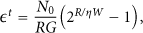
Based on these assumptions about link reliability and interference, we can abstract and approximate the service capability of a node by a deterministic service curve with the idea of effective transmission rate. From information theory, the Shannon capacity of a wireless channel can be expressed as $C=W\hspace{0.17em}{\log \hspace{0.17em}}_2(1+GP/N_0)$ , where $W,G,N_0$ are the same as those in (1). The service rate is defined as the rate that the information can be reliably transmitted. With an optimal or suboptimal channel coding scheme, a service rate of $R=\eta ·C$ can be guaranteed for any $0<\eta <1$ [29]. R defines a lower bound on the transmission rate. Therefore, the rate-latency service curve $\beta (t)={\chi }_{R,T}=R[t-T{]}^{+}$ can be applied to model the service capability of a wireless channel, where T denotes the maximum possible processing/queueing delay.

3.4. Delay, Backlog, and Output Bounds

Given the arrival curve and service curve of a node, the least upper delay bound, least upper backlog bound, and output bounds can be derived according to network calculus [11]. The least upper backlog bound is defined as the minimum value of the upper backlog bound. Consider a node i provides a service curve ${\beta }_i^s$ to the input flow which is constrained by an arrival curve ${\alpha }_i$ . According to network calculus, the least upper delay bound of the flow can be computed by

$\begin{array}{c}{D}_i=h\left({\alpha }_i,{\beta }_i^s\right)=\underset{t\ge 0}{\sup }\left\{\underset{\tau \ge 0}{\inf }\left\{\tau :{\alpha }_i\left(t\right)\le {\beta }_i^s\left(t+\tau \right)\right\}\right\}.\end{array}$

(4)

Moreover, the least upper backlog bound of node i can be calculated by

$\begin{array}{c}{B}_i=v\left({\alpha }_i,{\beta }_i^s\right)=\underset{t\ge 0}{\sup }\left\{{\alpha }_i\left(t\right)-{\beta }_i^s\left(t\right)\right\}.\end{array}$

(5)

Additionally, the arrival curve of the departure flow can be derived by

$\begin{array}{c}{\tilde{\alpha }}_i={\alpha }_i\oslash {\beta }_i^s=\underset{\tau \ge 0}{\sup }\left\{{\alpha }_i\left(t+\tau \right)-{\beta }_i^s\left(\tau \right)\right\}.\end{array}$

(6)

4. Analysis of the Flow-Based Traffic Splitting Strategy

In this section, we first introduce the splitting and multiplexing models. Then, the formal performance analysis procedure is presented. After that, we discuss the scope and assumptions of our analysis approach.

4.1. The Splitting Model

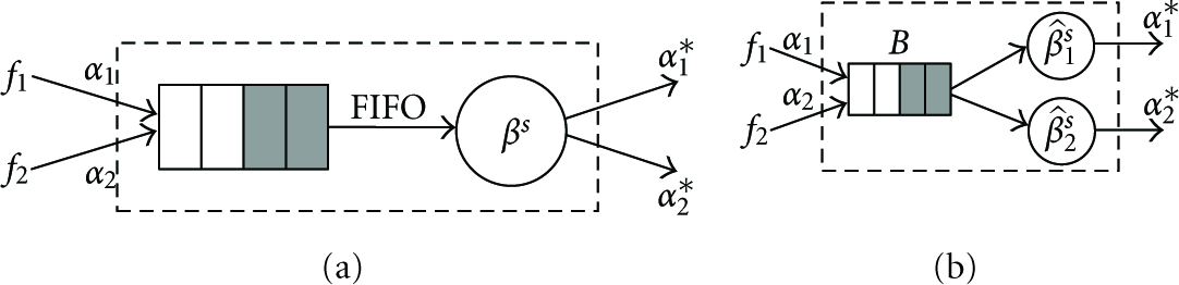
To analyze the splitting strategy, we build a splitting model that identifies the relations of input, output, delay, and backlog for a single node. Without losing generality, we consider a main flow is split into two subflows. The node $f_1$ traverse is abstracted as the combination of a buffer plus a splitter depicted in Figure 4(a).

Figure 4

(a) The main flow $f_1$ is split into two subflows $f_{1.1}$ and $f_{1.2}$ . (b) The equivalent model.

We consider that the node performs a weighted proportional splitting scheme, in which the main flow is split according to the configured weights, ${\varphi }_i$ for subflow i. In each round, the splitter will try to forward ${\varphi }_i$ packets to output link i before moving to the next one. The values of ${\varphi }_i$ can be set either according to a predefined rule or randomly. Increasing the value of ${\varphi }_i$ can result in increased packets to output link i. By adjusting ${\varphi }_i$ , the amount of traffic over each link can be controlled. If the service rate is R bits/s, the maximum length of a round is consequently equal to ${\sum }_i{\varphi }_{i}l/R$ seconds and the time for packets of subflow i to be forwarded within a round is bounded by ${\varphi }_{i}l/R$ seconds, where l is the packet length. In the weighted proportional splitting scheme, the worst case appears when the packets of a subflow just misses its turn in the current round. Consequently, it will have to wait for its turn at the next round. In the worst case, packets of the subflow i have to wait up to ${\sum }_{i\ne j}{\varphi }_{j}l/R$ seconds to be served.

Consider a main flow $f_1$ that is upper constrained by arrival curve ${\alpha }_1={\gamma }_{{\sigma }_1,{\rho }_1}$ , be split into two subflows $f_{1.1}$ and $f_{1.2}$ according to weights ${\varphi }_1$ and ${\varphi }_2$ , where ${\sigma }_1$ and ${\rho }_1$ denote the burstiness and average data rate of $f_1$ , respectively. Burstiness is defined as the amount of data inputted/outputted to/from a system or a node at one time. Consequently, it should be equal or bigger than the packet size l. Let ${\alpha }_{1.1}={\gamma }_{{\sigma }_{1.1},{\rho }_{1.1}}$ and ${\alpha }_{1.2}={\gamma }_{{\sigma }_{1.2},{\rho }_{1.2}}$ denote the arrival curves of $f_{1.1}$ and $f_{1.2}$ , respectively. Then, we have

$\begin{array}{c}{\rho }_{1.1}=\frac{{\varphi }_1}{{\varphi }_1+{\varphi }_2}{\rho }_1,\hspace{1em}\hspace{1em}{\sigma }_{1.1}=\max \left(\lceil \frac{{\varphi }_1{\sigma }_1}{({\varphi }_1+{\varphi }_2)l}\rceil \cdot l,l\right),\\ {\rho }_{1.2}=\frac{{\varphi }_2}{{\varphi }_1+{\varphi }_2}{\rho }_1,\hspace{1em}\hspace{1em}{\sigma }_{1.2}=\max \left(\lceil \frac{{\varphi }_2{\sigma }_1}{({\varphi }_1+{\varphi }_2)l}\rceil \cdot l,l\right),\end{array}$

(7)

where $\lceil ·\rceil$ denotes the minimum integer equal to or bigger than the number inside.

Let the splitter provide a service curve ${\beta }^s={\chi }_{R,T}$ . Since the splitter serves a subflow at one time, the service rate for each subflow also equals R. Therefore, the equivalent service curve for subflow $f_{1.1}$ can be derived by

$\begin{array}{c}{\widehat{\beta }}_1^s={\beta }^s\otimes {\delta }_{{\varphi }_{2}l/R}={\chi }_{R,T+{\varphi }_{2}l/R}.\end{array}$

(8)

Analogously, the equivalent service curve for $f_{2.2}$ is

$\begin{array}{c}{\widehat{\beta }}_2^s={\beta }^s\otimes {\delta }_{{\varphi }_{1}l/R}={\chi }_{R,T+{\varphi }_{1}l/R}.\end{array}$

(9)

Furthermore, the equivalent bounds on backlogs can be calculated by

$\begin{array}{c}{B}_1={\sigma }_{1.1}+\frac{{\varphi }_1{\rho }_1}{{\varphi }_1+{\varphi }_2}\left(T_1+\frac{{\varphi }_{2}l}{R}\right),\\ B_2={\sigma }_{1.2}+\frac{{\varphi }_2{\rho }_1}{{\varphi }_1+{\varphi }_2}\left(T_1+\frac{{\varphi }_{1}l}{R}\right).\end{array}$

(10)

Therefore, the least upper bound of the total backlog is computed by

$\begin{array}{c}B=B_1+B_2={\sigma }_1+{\rho }_1\left[T+\frac{2{\varphi }_1{\varphi }_{2}l}{R({\varphi }_1+{\varphi }_2)}\right].\end{array}$

(11)

The least upper delay bounds consist of three parts: the processing time, the time to serve input burstiness, and the scheduling delay. Let $D_{1.1}$ and $D_{1.2}$ denote the delay bounds of subflow $f_{1.1}$ and $f_{1.2}$ , respectively. They can be computed by

$\begin{array}{c}{D}_{1.1}=T+\frac{{\sigma }_{1.1}}{R}+\frac{{\varphi }_{2}l}{R},\hspace{1em}\hspace{1em}{D}_{1.2}=T+\frac{{\sigma }_{1.2}}{R}+\frac{{\varphi }_{1}l}{R}.\end{array}$

(12)

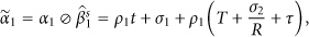
Furthermore, the departure arrival curves of $f_{1.1}$ and $f_{1.2}$ can be derived by

$\begin{array}{c}{\tilde{\alpha }}_{1.1}=\frac{{\varphi }_1{\rho }_1}{{\varphi }_1+{\varphi }_2}t+{\sigma }_{1.1}+\frac{{\varphi }_1}{{\varphi }_1+{\varphi }_2}\left({\rho }_{1}T+\frac{{\rho }_1{\varphi }_{2}l}{R}\right),\\ {\tilde{\alpha }}_{1.2}=\frac{{\varphi }_2{\rho }_1}{{\varphi }_1+{\varphi }_2}t+{\sigma }_{1.2}+\frac{{\varphi }_2}{{\varphi }_1+{\varphi }_2}({\rho }_{1}T+\frac{{\rho }_1{\varphi }_{1}l}{R}).\end{array}$

(13)

4.2. The Multiplexing Model

In order to analyze resource sharing when multiple input flows share the bandwidth of a link at a node, we propose a multiplexing model. We shall use this model for analyzing a network with various traffic flowing scenarios.

Without loss of generality, let us consider a node serve two flows $f_1$ and $f_2$ in the FIFO order as shown by Figure 5(a). And its equivalent model is drawn in Figure 5(b). Let the node provide a service curve ${\beta }^s$ to the aggregating flows, and $f_1$ and $f_2$ have ${\alpha }_1$ and ${\alpha }_2$ as arrive curves, respectively. We define ${\widehat{\beta }}_1^s=\kappa ({\beta }^s,{\alpha }_2)$ as the equivalent service curve [17] provided to flow $f_1$ , where $\kappa (·,·)$ is an operator to compute the equivalent service and τ is an intermediate argument. Thus, the departure arrival curve of $f_1$ can be derived by ${\tilde{\alpha }}_1={\alpha }_1\oslash \kappa ({\beta }^s,{\alpha }_2)$ , and its least upper delay bound is computed by $h({\alpha }_1,\kappa ({\beta }^s,{\alpha }_2))$ , and the least upper backlog bound of the node is $v({\alpha }_{\{\mathrm{1,2}\}},{\beta }^s)$ , where ${\alpha }_{\{\mathrm{1,2}\}}$ denotes the arrival curve of the aggregating flow $f_{\{\mathrm{1,2}\}}$ . Similarly, the equivalent service curve provides to flow $f_2$ can be derived by ${\widehat{\beta }}_2^s=\kappa ({\beta }^s,{\alpha }_1)$ , and its delay and backlog bounds, and departure arrival curve can be derived accordingly.

Figure 5

(a) A node serves two input flows. (b) The equivalent model.

We give an example to show how to compute $\kappa (·,·)$ . Let ${\beta }^s(t)={\chi }_{R,T}=R[t-T{]}^{+}$ and ${\alpha }_2(t)={\gamma }_{{\sigma }_2,{\rho }_2}(t)={\rho }_{2}t+{\sigma }_2$ , then, applying Corollary  4.5 in [17], the equivalent service curve for $f_1$ can be calculated by

$\begin{array}{c}{\widehat{\beta }}_1^s=\kappa ({\beta }^s,{\alpha }_2)={\gamma }_{R\cdot \tau ,R-{\rho }_2}\otimes {\delta }_{T+{\sigma }_2/R+\tau }\hspace{1em}(\tau \ge 0)\end{array},$

(14)

where τ is an intermediate argument for calculating the least upper delay bound, and ${\delta }_T(t)=+\infty$ for $t>T$ , and 0 otherwise.

The least upper delay bound of $f_1$ is calculated by

$\begin{array}{c}{D}_1=h\left({\alpha }_1,{\widehat{\beta }}_1^s\right)=\underset{\tau \ge 0}{\inf }\left\{T+\frac{{\sigma }_2}{R}+\frac{{\sigma }_1-R\tau }{R-{\rho }_2}+\tau \right\}.\end{array}$

(15)

Furthermore, the least upper backlog bound of the node can be derived by

$\begin{array}{c}B={\sigma }_1+{\sigma }_2+\left({\rho }_1+{\rho }_2\right)T.\end{array}$

(16)

Additionally, the arrival curve of the departure flow of $f_1$ is computed by

$\begin{array}{c}{\tilde{\alpha }}_1={\alpha }_1\oslash {\widehat{\beta }}_1^s={\rho }_{1}t+{\sigma }_1+{\rho }_1\left(T+\frac{{\sigma }_2}{R}+\tau \right),\end{array}$

(17)

where τ is the same as the value obtained in (15).

4.3. The Splitting-Based Performance Analysis Procedure

There have been several research works on the traffic splitting strategy in packet networks [6, 7], due to its efficiency in load balancing. In the flow-based splitting strategy, a traffic flow is split into multiple subflows at its source node, and these subflows are forwarded to the sink through different routing paths. The source node decides how the subflows are split. Given the traffic patterns, service models, the routing protocols, and the splitting strategy, we then detail the general performance analysis procedure as follows.

Step 1.

Based on the traffic pattern, routing protocols, and the traffic splitting strategy, construct a performance analysis model that converts the original network into an equivalent network.

Step 2.

Derive the input and departure arrival curves of all nodes in the network based on network calculus.

Step 3.

Derive the end-to-end equivalent service curves for the subflows; then compute the end-to-end least upper delay bound for the main flow using $D=h(\alpha ,\widehat{\beta })$ , where α denotes the input arrival curve and $\widehat{\beta }$ denotes the end-to-end equivalent service curve.

Step 4.

Using the results in Step  2, compute the least upper backlog bound of each node $B_s=v({\sum }_{i\in ℐ(s)}{\alpha }_i^s,{\beta }^s)$ , where $ℐ(s)$ represents the set of input flows of node s.

Step 5.

Compute the power consumption of a node s by $P_s={ϵ}^r{\sum }_{i\in N_{\text{in}}(s)}{\rho }_{is}+{\sum }_{j\in N_{\text{out}}(s)}{ϵ}_{sj}^t{\rho }_{sj}+p_s^c$ , where $N_{\text{in}}(i)$ and $N_{\text{out}}(i)$ denote the set of nodes which are the direct sources of incoming data flows and the direct destinations of output data flows of node i, respectively.

4.4. Discussions

4.4.1. Flow-Based Splitting versus Multipath Routing

Basically, a traffic splitting process consists of two stages: establishing multiple routing paths and allocating traffic on each path according to the splitting strategy. Multipath routing is a technique exploiting routing diversity by using multiple source-destination pairs. It has been receiving plenty of research attentions [33, 34]. There are plenty of works in the literature on how to set up multiple routing paths in ad hoc networks [18, 34, 35]. Our work focuses on analyzing the performance of the splitting strategy rather than finding multipath routes. We assume that multiple paths have already been established between source nodes and the sink.

There are several common features between multipath routing and flow-based traffic splitting: first, both of them use multipaths to explore routing diversities; second, both of them aim for improving load balance. Apart from these common features, there exist significant differences between them. In multipath routing, routing decisions are made on a per-packet basis, this is, each packet chooses its routing path and is forwarded to the destination individually. Multipath routing is mainly used for improving network performance in terms of reliability and robustness [33, 34]. While in flow-based splitting strategy, the routing and forwarding is made on a per-flow basis. So it is capable of realizing a controlled splitting and providing quality of service. For example, if there are two paths between a source and a destination, a flow may be split half to one path and half to the other. So the delay guarantees can be reasoned about.

4.4.2. Flow-Based Splitting versus Node-Based Splitting

According to the way that a traffic flow split, the traffic splitting strategy can be classified into two categories: flow-based splitting and node-based splitting.

In flow-based splitting, the source node decides how the subflows are scheduled and split. The subflows can be identified after splitting. As shown in Figure 6(a), the traffic flow $f_i$ is split into two subflows ( $f_{i.1}$ and $f_{i.2}$ ) only at its source node $s_1$ and forwarded to the sink ( $s_6$ ) through two routing paths: $\{s_1,s_2,s_4\}$ and $\{s_1,s_3,s_5\}$ . In the node-based traffic splitting strategy (Figure 6(b)), the traffic flow can be split at the intermediate nodes that have multiple output links (such as nodes $s_1$    $s_2$    $s_3$ in Figure 6(b)), and these nodes decide how their input flows are allocated to their output links. An example of node-based routing strategy is the backpressure-based routing protocol (BCP) [23]. Implementing a flow-based traffic splitting strategy is more complex than a node-based traffic splitting strategy in practice, but a flow-based traffic splitting strategy also has its own advantages. In the flow-based splitting strategy, the routing and forwarding decisions are made on a per-flow basis. So it is capable of realizing a controlled splitting and satisfying quality of service requirements.

Figure 6

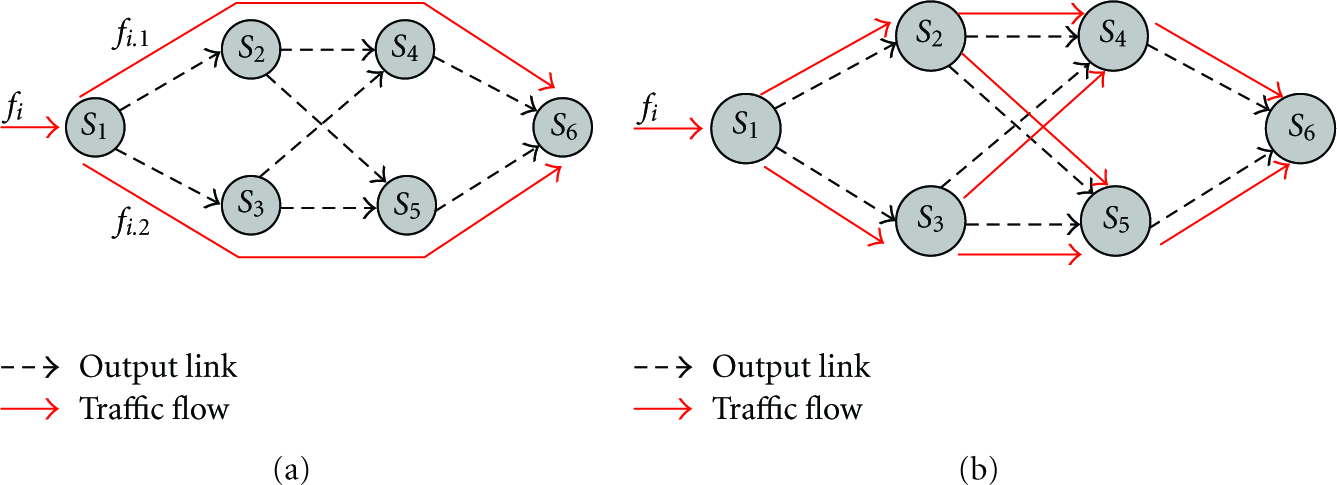
An example of splitting strategies. $s_1$ is the source node of the traffic flow, and $s_6$ is the sink. (a) Flow-based traffic splitting strategy; (b) node-based traffic splitting strategy.

4.4.3. How to Set Splitting Parameters?

Our work mainly provides a framework for quality of service analysis of the flow-based splitting strategy. Another research issue is on splitting parameter exploration, that is, how to set splitting factors? One way is to utilize static network state information, such as link capacity and buffer length, to set splitting parameters. For example, in Figure 6(a), source node $S_1$ can select appropriate splitting factors based on the link capacity information of it downstream links. A larger amount of traffic can be allocated to the links with higher capacity. In [36], authors presented an explicit rate-based flow control scheme, in which each route ran a proportional max-min fair bandwidth sharing algorithm to divide the measure bandwidth among the passed flows. Alternatively, the splitting decision can be made based on dynamical network state information. Each node records its current or historic buffer lengths, and the information is sent to the source node, so that the source node can select appropriate splitting parameters. For example, authors in [37] proposed a congestion-aware routing scheme which could redirect a certain amount of traffic to other paths under heavy traffic load. In this scheme, the congestion status information at each route is detected depending on the average MAC layer utilization and queue length. If congestion happens, traffic is split into other paths according to its services type.

5. An Analysis Example

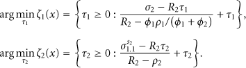
In this section, we exemplify the general performance analysis and derive close-form formulas for of delay bounds, backlog bounds, and power consumptions under the conditions of affine arrival curve and rate-latency service curve. Consider a network consists of four nodes as shown in Figure 7. We define the tagged main flow as the main flow for which we shall derive the end-to-end delay bound. In this example, we choose $f_1$ as the tagged main flow. Let $f_1$ be constrained by the arrival curve ${\alpha }_1={\gamma }_{{\sigma }_1,{\rho }_1}$ , and split into two subflows $f_{1.1}$ and $f_{1.2}$ and, respectively, traverse two different routing paths $ℛ(f_{1.1})=\{s_1,s_2,s_4\}$ and $ℛ(f_{1.2})=\{s_1,s_3,s_4\}$ from the source node $s_1$ to the sink. ${\varphi }_1$ and ${\varphi }_2$ are the splitting weights of $f_{1.1}$ and $f_{1.2}$ , respectively. $f_2$ is the contention flow that is modeled by the arrival curve ${\alpha }_2={\gamma }_{{\sigma }_2,{\rho }_2}$ . Let ${\alpha }_j^{s_i}$ and ${\tilde{\alpha }}_j^{s_i}$ , respectively, denote the input and departure arrival curves of flow j at node $s_i$ . Next, we need to derive the end-to-end least upper delay bound for flow $f_1$ and the least upper backlog bound and power consumption for each node.

Figure 7

(a) A network analysis example: the main flow $f_1$ is split into two subflows $f_{1.1}$ and $f_{1.2}$ . $f_2$ is the contention flow. (b) The equivalent analysis network: the blue, green, and red dashed lines show the routing path of flow $f_{1.1}$ , $f_{1.2}$ , and $f_2$ , respectively.

In order to compute the end-to-end least upper delay and the least upper backlog bounds, we first need to derive the input and departure arrival curves of each node.

5.1. Arrival Curves of Input and Output

According to the results of the splitting model, the arrival curves of departure flows at node $s_1$ can be derived as

$\begin{array}{cc}\hfill & {\tilde{\alpha }}_{1.1}^{s_1}=\frac{{\varphi }_1{\rho }_1}{{\varphi }_1+{\varphi }_2}t+{\sigma }_{1.1}+\frac{{\varphi }_1}{{\varphi }_1+{\varphi }_2}\left({\rho }_1{T}_1+\frac{{\rho }_1{\varphi }_{2}l}{R_1}\right),\hfill \\ \hfill & {\tilde{\alpha }}_{1.2}^{s_1}=\frac{{\varphi }_2{\rho }_1}{{\varphi }_1+{\varphi }_2}t+{\sigma }_{1.2}+\frac{{\varphi }_2}{{\varphi }_2}\left({\sigma }_1+{\rho }_1{T}_1+\frac{{\rho }_1{\varphi }_{1}l}{R_1}\right).\hfill \end{array}$

(18)

Node $s_2$ has two input flows, with arrival curves ${\alpha }_2$ and ${\alpha }_{1.1}^{s_2}={\tilde{\alpha }}_{1.1}^{s_1}$ . According to the multiplexing analysis results (Section 4.2), we can derive the arrival curves of the departure flows of node $s_2$ as following

$\begin{array}{cc}\hfill & {\tilde{\alpha }}_2^{s_2}={\rho }_{2}t+{\sigma }_2+{\rho }_2\left(T_2+\frac{{\sigma }_{1.1}^{s_2}}{R_2}+{\tau }_1\right),\hfill \\ \hfill & {\tilde{\alpha }}_{1.1}^{s_2}={\tilde{\alpha }}_{1.1}^{s_1}+\frac{{\varphi }_1{\rho }_1}{{\varphi }_1+{\varphi }_2}\left(T_2+\frac{{\sigma }_2}{R_2}+{\tau }_2\right),\hfill \end{array}$

(19)

where ${\sigma }_{1.1}^{s_2}={\sigma }_{1.1}+({\varphi }_1/({\varphi }_1+{\varphi }_2))({\rho }_1{T}_1+{\rho }_1{\varphi }_{2}l/R_1)$ , ${\tau }_1$ and ${\tau }_2$ are defined by

$\begin{array}{cc}\hfill & \arg \underset{{\tau }_1}{\min }\hspace{0.17em}{\zeta }_1\left(x\right)=\left\{{\tau }_1\ge 0:\frac{{\sigma }_2-R_2{\tau }_1}{R_2-{\varphi }_1{\rho }_1/({\varphi }_1+{\varphi }_2)}+{\tau }_1\right\},\hfill \\ \hfill & \arg \underset{{\tau }_2}{\min }\hspace{0.17em}{\zeta }_2\left(x\right)=\left\{{\tau }_2\ge 0:\frac{{\sigma }_{1.1}^{s_2}-R_2{\tau }_2}{R_2-{\rho }_2}+{\tau }_2\right\}.\hfill \end{array}$

(20)

For node $s_3$ , the arrival curve of its input flow is ${\alpha }_{1.2}^{s_3}={\tilde{\alpha }}_{1.2}^{s_1}$ , and it provides a service curve ${\beta }^{s_3}={\chi }_{R_3,T_3}$ . Consequently, the arrival curve of its departure flow is

$\begin{array}{c}{\tilde{\alpha }}_{1.2}^{s_3}={\tilde{\alpha }}_{1.2}^{s_1}+\frac{{\varphi }_2{\rho }_1}{{\varphi }_1+{\varphi }_2}{T}_3.\end{array}$

(21)

According to the connection relations, we can get the arrival curves of three input flows at node $s_4$ , which are ${\alpha }_2^{s_4}={\tilde{\alpha }}_2^{s_2}$ , ${\alpha }_{1.1}^{s_4}={\tilde{\alpha }}_{1.1}^{s_2}$ , and ${\alpha }_{1.2}^{s_4}={\tilde{\alpha }}_{1.2}^{s_3}$ . Since it is not necessary to compute the arrival curves of the departure flows at node $s_4$ , we omit the derivation here.

5.2. The End-to-End Delay Bound

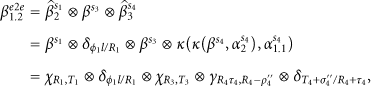
In order to compute the end-to-end delay bound, we first need to derive the service curve provided by individual nodes. Let ${\widehat{\beta }}_k^{s_i}$ represent the equivalent service curve provided by node $s_i$ to its kth input flow. As shown in Figure 7, node $s_2$ serves two flow $f_{1.1}$ and $f_2$ . According to the multiplexing analysis in Section 4.2, the equivalent service curve for $f_{1.1}$ at $s_2$ is ${\widehat{\beta }}_2^{s_2}=\kappa ({\beta }^{s_2},{\alpha }_2)$ . Node $s_4$ serves three flows, and the equivalent service curve for $f_{1.1}$ is ${\widehat{\beta }}_1^{s_4}=\kappa (\kappa ({\beta }^{s_4},{\alpha }_2^{s_4}),{\alpha }_{1.2}^{s_4})$ . Thus, the end-to-end equivalent service curve for $f_{1.1}$ can be derived by

$\begin{array}{cc}\hfill {\beta }_{1.1}^{e2e}& ={\widehat{\beta }}_1^{s_1}\otimes {\widehat{\beta }}_2^{s_2}\otimes {\widehat{\beta }}_2^{s_4}\hfill \\ \hfill & ={\beta }^{s_1}\otimes {\delta }_{{\varphi }_{2}l/R_1}\otimes \kappa ({\beta }^{s_2},{\alpha }_2)\otimes \kappa (\kappa ({\beta }^{s_4},{\alpha }_2^{s_4}),{\alpha }_{1.2}^{s_4})\hfill \\ \hfill & ={\chi }_{R_1,T_1}\otimes {\delta }_{{\varphi }_{2}l/R_1}\otimes {\gamma }_{R_2{\tau }_2,R_2-{\rho }_2}\otimes {\delta }_{T_2+{\sigma }_2/R_2+{\tau }_2}\otimes {\gamma }_{R_4{\tau }_3,R_4-{\rho }_4^{\prime }}\hfill \\ \hfill & \hspace{1em}\otimes {\delta }_{T_4+{\sigma }_4^{\prime }/R_4+{\tau }_3}\hfill \\ \hfill & ={\chi }_{R_1,T_1}\otimes {\delta }_{{\varphi }_{2}l/R_1+T_2+{\sigma }_2/R_2+{\tau }_2+T_4+{\sigma }_4^{\prime }/R_4+{\tau }_3}\otimes {\gamma }_{R_2{\tau }_2,R_2-{\rho }_2}\hfill \\ \hfill & \hspace{1em}\otimes {\gamma }_{R_4{\tau }_3,R_4-{\rho }_4^{\prime }},\hfill \end{array}$

(22)

where ${\tau }_1$ and ${\tau }_2$ are the same as those in (19), ${\tau }_3$ is calculated by $\arg {\min \hspace{0.17em}}_{{\tau }_3}\{{\tau }_3\ge 0:({\sigma }_{1.1}^{s_4}-R_4{\tau }_3)/(R_4-{\rho }_4^{\prime })+{\tau }_3\}$ , ${\rho }_4^{\prime }={\rho }_2+{\varphi }_2{\rho }_1/({\varphi }_1+{\varphi }_2)$ and

$\begin{array}{cc}\hfill {\sigma }_4^{\prime }& ={\rho }_2(T_2+\frac{{\sigma }_{1.1}^{s_2}}{R_2}+{\tau }_1)+{\sigma }_{1.2}\hfill \\ \hfill & \hspace{1em}+\frac{{\varphi }_2\left[{\rho }_1\left(T_1+T_3\right)+{\rho }_1{\varphi }_{1}l/R_1\right]}{{\varphi }_1+{\varphi }_2}+{\sigma }_2.\hfill \end{array}$

(23)

Analogously, the end-to-end equivalent service curve for $f_{1.2}$ can be derived by

$\begin{array}{cc}\hfill {\beta }_{1.2}^{e2e}& ={\widehat{\beta }}_2^{s_1}\otimes {\beta }^{s_3}\otimes {\widehat{\beta }}_3^{s_4}\hfill \\ \hfill & ={\beta }^{s_1}\otimes {\delta }_{{\varphi }_{1}l/R_1}\otimes {\beta }^{s_3}\otimes \kappa (\kappa ({\beta }^{s_4},{\alpha }_2^{s_4}),{\alpha }_{1.1}^{s_4})\hfill \\ \hfill & ={\chi }_{R_1,T_1}\otimes {\delta }_{{\varphi }_{1}l/R_1}\otimes {\chi }_{R_3,T_3}\otimes {\gamma }_{R_4{\tau }_4,R_4-{\rho }_4^{\mathrm{\prime \prime }}}\otimes {\delta }_{T_4+{\sigma }_4^{\mathrm{\prime \prime }}/R_4+{\tau }_4},\hfill \end{array}$

(24)

where ${\tau }_4$ is defined by $\arg {\min \hspace{0.17em}}_{{\tau }_4}\{{\tau }_4\ge 0:({\sigma }_{1.2}^{s_4}-R_4{\tau }_4)/(R_4-{\rho }_4^{\mathrm{\prime \prime }})+{\tau }_4\}$ , ${\rho }_4^{\mathrm{\prime \prime }}=({\rho }_2+{\varphi }_1{\rho }_1/({\varphi }_1+{\varphi }_2))$ and

$\begin{array}{cc}\hfill {\sigma }_4^{\mathrm{\prime \prime }}& =\frac{{\varphi }_1{\rho }_1}{{\varphi }_1+{\varphi }_2}(T_1+T_2+\frac{{\sigma }_2}{R_2}+{\tau }_2)+\frac{{\rho }_1{\varphi }_1{\varphi }_{2}l}{R_1({\varphi }_1+{\varphi }_2)}\hfill \\ \hfill & \hspace{1em}+{\rho }_2\left(T_2+\frac{{\sigma }_{1.1}^{s_2}}{R_2}+{\tau }_1\right)+{\sigma }_{1.1}+{\sigma }_2,\hfill \end{array}$

(25)

where ${\tau }_1$ and ${\tau }_2$ are the same as those in (19).

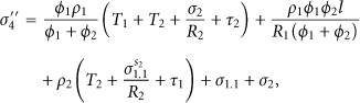
After we get the end-to-end service curves, the least upper delay bounds of $f_{1.1}$ and $f_{1.2}$ can be, respectively, computed by $h({\alpha }_{1.1},{\beta }_{1.1}^{e2e})$ and $h({\alpha }_{1.2},{\beta }_{1.2}^{e2e})$ ,

$\begin{array}{cc}\hfill & h({\alpha }_{1.1},{\beta }_{1.1}^{e2e})\hfill \\ \hfill & \hspace{1em}=T_1+T_2+T_4+\frac{{\varphi }_{2}l}{R_1}+\frac{{\sigma }_2}{R_2}+\frac{{\sigma }_4^{\prime }}{R_4}\hfill \\ \hfill & \hspace{1em}\hspace{1em}+\underset{\begin{array}{c}{\tau }_2\ge 0\\ {\tau }_3\ge 0\end{array}}{\inf }\{\phantom{\left[\frac{{\sigma }_{1.1}}{R_1}\vee \frac{{\sigma }_{1.1}-R_2{\tau }_2}{R_2-{\rho }_2}\vee \frac{{\sigma }_{1.1}-R_4{\tau }_3}{R_4-{\rho }_4^{\prime }}\right]}{\tau }_2+{\tau }_3+\left[\frac{{\sigma }_{1.1}}{R_1}\vee \frac{{\sigma }_{1.1}-R_2{\tau }_2}{R_2-{\rho }_2}\vee \frac{{\sigma }_{1.1}-R_4{\tau }_3}{R_4-{\rho }_4^{\prime }}\right]\},\hfill \\ \hfill & \hspace{1em}\hfill \\ \hfill & h\left({\alpha }_{1.2},{\beta }_{1.2}^{e2e}\right)\hfill \\ \hfill & \hspace{1em}=T_1+T_3+T_4+\frac{{\varphi }_{1}l}{R_1}+\frac{{\sigma }_4^{\mathrm{\prime \prime }}}{R_4}\mathrm{\hspace{0.17em}\hspace{0.17em}}\hfill \\ \hfill & \hspace{1em}\hspace{1em}+\underset{{\tau }_4\ge 0}{\inf }\left\{{\tau }_4+\left[\frac{{\sigma }_{1.2}}{R_1}\vee \frac{{\sigma }_{1.2}}{R_3}\vee \frac{{\sigma }_{1.2}-R_4{\tau }_4}{R_4-{\rho }_4^{\mathrm{\prime \prime }}}\right]\right\}.\hfill \end{array}$

(26)

Hence, the end-to-end least upper delay bound for the flow $f_1$ equals the maximum of the delays of two subflows, namely,

$\begin{array}{c}{D}_{f_1}=\max \left\{h({\alpha }_{1.1},{\beta }_{1.1}^{e2e}),h({\alpha }_{1.2},{\beta }_{1.2}^{e2e})\right\}.\end{array}$

(27)

5.3. The Backlog Bound

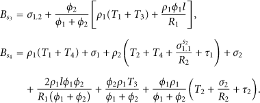
Let $B_{s_i}$ denote the backlog bound of node $s_i$ $(i=1,\dots ,4)$ . As we have already derived the arrival curves of input and output flows at each node, its least upper backlog bound can be calculated very easily. According to the result in (11), we have

$\begin{array}{c}{B}_{s_1}=B_{1.1}+B_{1.2}={\sigma }_1+{\rho }_1\left[T_1+\frac{2{\varphi }_1{\varphi }_{2}l}{R_1({\varphi }_1+{\varphi }_2)}\right].\end{array}$

(28)

Node $s_2$ has two input flows ${\alpha }_2$ and ${\alpha }_{1.1}^{s_2}$ , so its least upper backlog bound is computed by

$\begin{array}{c}{B}_{s_2}={\sigma }_{1.1}+{\sigma }_2+\frac{{\varphi }_1\left({\rho }_1{T}_1+{\rho }_1{\varphi }_{2}l/R_1\right)\mathrm{\hspace{0.17em}\hspace{0.17em}}}{{\varphi }_1+{\varphi }_2}+\left(\frac{{\varphi }_1{\rho }_1}{{\varphi }_1+{\varphi }_2}+{\rho }_2\right)T_2.\end{array}$

(29)

Analogously, the least upper backlog bounds of node $s_3$ and $s_4$ can be derived by

$\begin{array}{cc}\hfill B_{s_3}& ={\sigma }_{1.2}+\frac{{\varphi }_2}{{\varphi }_1+{\varphi }_2}\left[{\rho }_1(T_1+T_3)+\frac{{\rho }_1{\varphi }_{1}l}{R_1}\right],\hfill \\ \hfill B_{s_4}& ={\rho }_1(T_1+T_4)+{\sigma }_1+{\rho }_2\left(T_2+T_4+\frac{{\sigma }_{1.1}^{s_2}}{R_2}+{\tau }_1\right)+{\sigma }_2\hfill \\ \hfill & \hspace{1em}+\frac{2{\rho }_{1}l{\varphi }_1{\varphi }_2}{R_1\left({\varphi }_1+{\varphi }_2\right)}+\frac{{\varphi }_2{\rho }_1{T}_3}{{\varphi }_1+{\varphi }_2}+\frac{{\varphi }_1{\rho }_1}{{\varphi }_1+{\varphi }_2}\left(T_2+\frac{{\sigma }_2}{R_2}+{\tau }_2\right).\hfill \end{array}$

(30)

5.4. Power Consumption

According to the power model (Section 3.2), the total power consumption of a node is contributed by the radio transmitter, radio receiver, and computation electronics. Thus, the power consumptions of all the nodes can be computed by

$\begin{array}{cc}\hfill P_{s_1}& ={ϵ}^r{\rho }_1+{ϵ}_{s_1{s}_2}^t{\rho }_{1.1}+{ϵ}_{s_1{s}_3}^t{\rho }_{1.2}+p^c\hfill \\ \hfill & ={\rho }_1\left[{ϵ}^r+\frac{{\varphi }_1{N}_0\left(2^{R_{s_1{s}_2}/\eta W}-1\right)}{R_{s_1{s}_2}{G}_{s_1{s}_2}\left({\varphi }_1+{\varphi }_2\right)}+\frac{{\varphi }_2{N}_0\left(2^{R_{s_1{s}_3}/\eta W}-1\right)}{R_{s_1{s}_3}{G}_{s_1{s}_3}\left({\varphi }_1+{\varphi }_2\right)}\right]\hfill \\ \hfill & \hspace{1em}+p^c,\hfill \\ \hfill P_{s_2}& ={ϵ}^r\left({\rho }_{1.1}+{\rho }_2\right)+{ϵ}_{{\text{s}}_2{s}_4}^t\left({\rho }_{1.1}^{s_4}+{\rho }_2^{s_4}\right)+p^c\hfill \\ \hfill & =\left[{ϵ}^r+\frac{N_0\left(2^{R_{s_2{s}_4}/\eta W}-1\right)}{R_{s_2{s}_4}{G}_{s_2{s}_4}}\right]\left(\frac{{\varphi }_1{\rho }_1}{{\varphi }_1+{\varphi }_2}+{\rho }_2\right)+p^c,\hfill \\ \hfill P_{s_3}& =\left[{ϵ}^r+\frac{N_0\left(2^{R_{s_3{s}_4}/\eta W}-1\right)}{R_{s_3{s}_4}{G}_{s_3{s}_4}}\right]\frac{{\varphi }_2{\rho }_1}{{\varphi }_1+{\varphi }_2}+p^c,\hfill \\ \hfill P_{s_4}& =\left[{ϵ}^r+\frac{N_0\left(2^{R_{s_4{s}_0}/\eta W}-1\right)}{R_{s_4{s}_0}{G}_{s_4{s}_0}}\right]\left({\rho }_1+{\rho }_2\right)+p^c,\hfill \end{array}$

(31)

where $d_{s_4{s}_0}$ denotes the distance between node $s_4$ and the sink node $s_0$ . Here, we assume that the link capacity can meet the requirements of the traffic bandwidth, that is, the service rate is bigger than the sum of input data rates.

6. Performance Evaluation

To show benefits of the traffic splitting strategy and validate the network calculus-based performance analysis method, we provide numerical results and simulations under the scenario of a fresh food monitoring application. In the numerical results, the end-to-end least upper delay bounds, the least upper backlog bounds, and power consumptions are compared under two scenarios: general routing with no traffic splitting (NOS) and flow-based splitting strategy (FBS). In the simulations, we compare the results obtained by the analytical method with the simulation results also under these two scenarios.

The numerical results are based on an application example of a real-time fresh food monitoring system deployed in a warehouse [3, 4]. As shown in Figure 8, one sink and 9 cluster heads are uniformly distributed in a 20 m × 10 m warehouse. Each cluster head connects with 5 sensor nodes. The coordinates of cluster heads and sink ( $s_0$ ) are $s_0(\mathrm{0,0})$ , $s_1(\mathrm{17.2,1.7})$ , $s_2(\mathrm{14.1,5.5})$ , $s_3(\mathrm{11,0.5})$ , $s_4(14.8,-3.6)$ , $s_5(\mathrm{8.3,4})$ , $s_6(9.1,-4.4)$ , $s_7(\mathrm{2.5,4.7})$ , $s_8(\mathrm{4.2,0.8})$ , $s_9(3.3,-3.6)$ . We consider the application scenario of real-time monitoring, where sensor nodes periodically generate packets when there is a request.

Figure 8

A cluster-mesh sensor network: $s_0$ is the sink. An event happens in the blue circle, and three traffic flows $f_1$ , $f_2$ , $f_3$ are generated.

6.1. Numerical Results

Assume sensor nodes in cluster ${𝒞}_1,{𝒞}_2$ , and ${𝒞}_3$ are requested to send packets to the sink via cluster head $s_1$ , $s_2$ , and $s_3$ , respectively. Consequently, there are three traffic flows in the network: $f_1$ , $f_2$ , and $f_3$ . They are characterized by arrival curves ${\alpha }_1={\sum }_{n_j\in {𝒞}_1}{\alpha }_1^j$ , ${\alpha }_2={\sum }_{n_j\in {𝒞}_2}{\alpha }_2^j$ , ${\alpha }_3={\sum }_{n_j\in {𝒞}_3}{\alpha }_3^j$ , where ${\alpha }_i^j$ $(i=\mathrm{1,2},3)$ denotes the arrival curve of traffic generate by sensor node j in cluster ${𝒞}_i$ . For periodic packets generation applications, the arrival process can be characterized by the affine arrival curve [12], that is, ${\alpha }_1={\gamma }_{{\sigma }_1,{\rho }_1}$ , ${\alpha }_2={\gamma }_{{\sigma }_2,{\rho }_2}$ , and ${\alpha }_3={\gamma }_{{\sigma }_3,{\rho }_3}$ . Moreover, assume cluster head $s_i$ provides a rate-latency service curve ${\beta }^{s_i}={\chi }_{R_i,T_i}$ . $f_1$ is the tagged main flow, and $f_2$ , $f_3$ are the contention flows. Other parameters are listed in Table 1. We shall derive the end-to-end least upper delay bound for $f_1$ , the least upper backlog bounds, and power consumptions of all nodes in two scenarios: NOS and FBS (Figure 9).

Table 1

Parameters.

Parameter	Notation	Value	Unit
Packet length	l	400	bits
Computation power	$p^c$	10	uJ/s
Path loss factor	θ	3	—
Service delay	$T_i\mathrm{\hspace{0.17em}\hspace{0.17em}}(i=1,\dots ,9)$	0.1	s
Data rate of $f_2$	${\rho }_2$	1.2	kbps
Data rate of $f_3$	${\rho }_3$	1.6	kbps
Burstiness	${\sigma }_1,{\sigma }_2,{\sigma }_3$	400	bits
Channel bandwidth	W	20	kHz

Figure 9

(a) General routing with no splitting (NOS): the tagged main flow $f_1$ chooses one of path 1, 2, or 3, and the routing paths of $f_2$ and $f_3$ are shown by the blue and green line, respectively. (b) Flow-based splitting (FBS): all three flows are split as shown by the red, blue, and green lines, respectively.

From the power model in (1) and Figure 2, the energy per bit is a monotonically increasing function of the transmission rate [29] if other parameters are fixed. Thus, it is better to use low transmission power for the sake of energy efficiency. On the other hand, the delay bound is a monotonically decreasing function of the service rate. (e.g., given an arrival curve $\alpha (t)=\rho t+\sigma$ and service curve $\beta (t)=R[t-T{]}^{+}$ , the delay bound is $T+\sigma /R$ when $R\ge \rho$ .) Therefore, there is a tradeoff between energy consumption and delay. In order to study this tradeoff, we implement numerical experiments in two scenarios: (1) uniform service rate: the service rate of all cluster heads are the same and fixed; (2) heterogeneous service rate: in order to guarantee a limited delay and backlog, the service rate should be equal to or bigger than the data arrival rate. So we set the service rate R equal to the arrival rate ρ.

We compare the end-to-end least upper delay of $f_1$ , the backlog bounds, and power consumptions of all nodes in two scenarios: NOS and FBS. In NOS, $f_1$ chooses one of the three paths: path 1— $\{s_1,s_3,s_8\}$ , path 2— $\{s_1,s_4,s_6,s_9\}$ , and path 3— $\{s_1,s_2,s_5,s_7\}$ . In FBS, $f_1$ is evenly split into three subflows, and they are allocated on these three paths.

6.1.1. Uniform Service Rate

In the first numerical example, we choose a fixed service rate $\mathrm{\hspace{0.17em}\hspace{0.17em}}{R}_i=9.6$  kbps   $(i=1,\dots ,9)$ .

Figure 10 shows the comparison of the end-to-end least upper delay bounds of the tagged main flow $f_1$ in NOS and FBS scenarios. In the NOS scenario, we compute the end-to-end delays of $f_1$ going through three different routing paths (Figure 9(a)). The input data rate of $f_1$ varies from 1.2 kbps to 4 kbps. From this figure, we can see that the end-to-end delays in all scenarios increase with the input data rates. Furthermore, on average, the delays in FBS are 23.6% and 9.4% less than those of path 2 and path 3 in NOS, respectively. And the delay in FBS is 12.4% bigger than those of path 1 in NOS. This is because path 1 is shorter than other two paths.

Figure 10

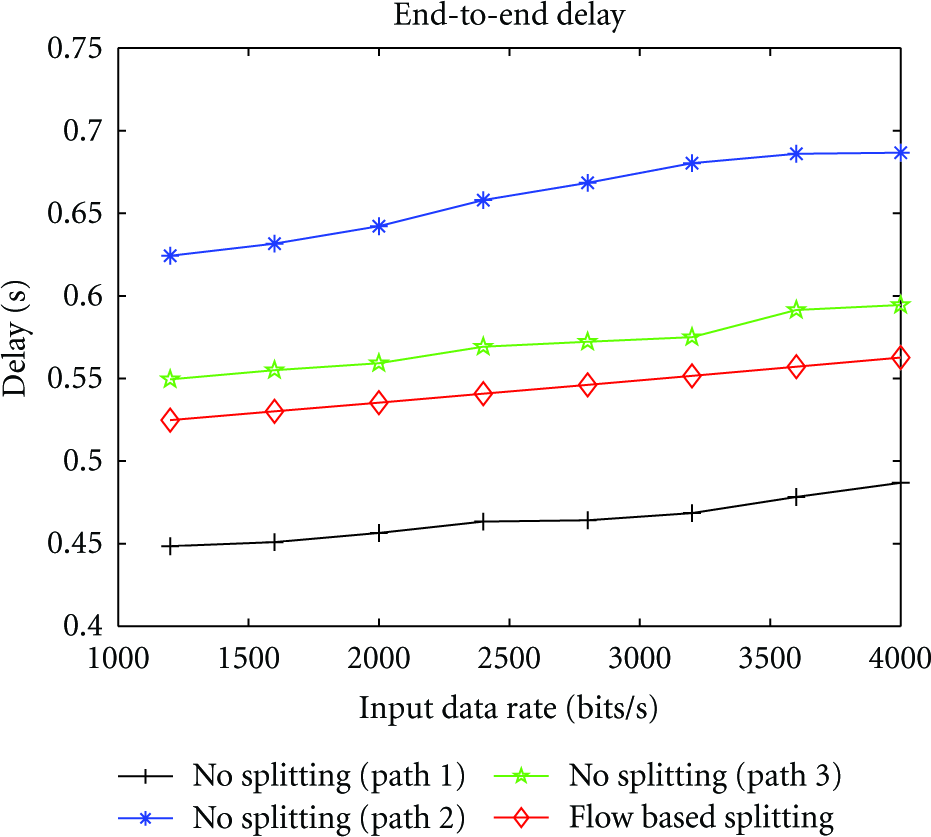
End-to-end least upper delay bound.

Figure 11 shows the least upper and average backlog bounds in the FBS and NOS scenarios with input data rates vary, where “Max-B(NOS)” means the maximum backlog in NOS which denotes the maximum value of backlogs among all nodes and “Ave-B(FBS)” means the average backlog in FBS which denotes the average value of backlogs over all nodes. From this figure, we can find that both the maximum and average backlogs in FBS are less than those in NOS. It indicates that the traffic splitting strategy can reduce backlogs. Moreover, the differences between the maximum backlogs of the two scenarios are much bigger than those of average backlogs. The average backlogs in FBS are 14.5% less than those in NOS on the average. While the maximum backlog in FBS is 23.4% less than that in NOS when the input data rate is 1.2 kbps, and the value increases to 40% when the input data rate is 4 kbps. We can also observe similar reduction in the variance of maximum backlogs (as shown in Figure 12), where the variance of backlogs in NOS is much bigger than that in FBS. It means that in NOS some nodes have very small backlogs, but some nodes have very large backlogs. Since the buffer size of a sensor node is basically determined by the value of maximum backlog, larger backlog would bring higher hardware cost. Therefore, applying the flow-based splitting strategy can bring better load balance and thus reduce overall cost.

Figure 11

Least upper backlog bounds (in NOS: flow 1 chooses path 3).

Figure 12

Variance of least upper backlog bounds (in NOS: flow 1 chooses path 3).

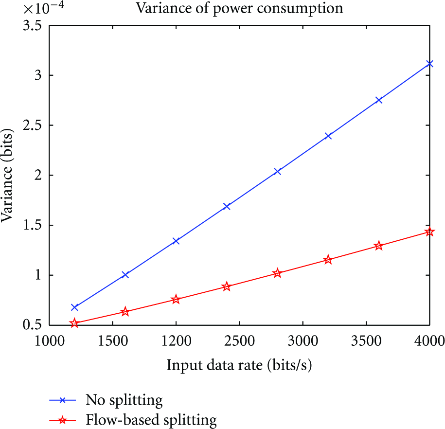
The maximum and average power consumptions of all nodes in NOS and FBS are shown in Figure 13, where “Max-P(NOS)” and “Ave-B(NOS),” respectively, denote the maximum and average power consumptions in the NOS scenario. First, we see from the figure that all the power consumptions increase with the input data rates. Furthermore, when the data rate increases, the average power consumptions in the NOS and FBS are almost the same. However, the maximum power consumption in NOS increases much faster than that in FBS, with the maximum differences between FBS and NOS increasing from 0.8% to 12%. It indicates that the power consumptions of nodes are uneven in NOS. We can also see this from Figure 14 showing the variance of power consumption of all nodes. From this figure, we can find the variance in NOS increases much faster than that in FBS. Usually, the lifetime of a WSN is determined by the first node exhausting its energy. Hence, the flow-based splitting scheme can be used for balancing power consumption and consequently increasing the lifetime of the network.

Figure 13

Power consumption (In NOSi: flow 1 chooses path i, where $i=\mathrm{1,2},3$ ).

Figure 14

Variance of power consumption.

6.1.2. Heterogeneous Service Rate

The data rate of $f_1$ varies from 1.2 to 4 kbps. The data rate of $f_2$ and $f_3$ is given in Table 1. The service rate of each node is equal to its arrival rate.

Being different from Figure 10, the end-to-end delays of FBS are basically bigger than those of NOS in this case (Figure 15). Moreover, when the input data rate increases, the end-to-end delay decreases. The reason is that the service rate increases with the input data rate. While the input burstiness is the same, so the delay would decrease.

Figure 15

End-to-end delay.

Figure 16 shows the comparison of backlog bounds in the FBS and NOS scenarios. From this figure, we can find that the average backlogs in FBS and NOS are almost the same. While the maximum backlog in FBS is −2.4% less than that in NOS when the input data rate is 1.2 kbps, the value gradually increases to 12.8% when the input data rate gradually increases to 4 kbps. Similar to Figure 12, from Figure 17, we can see that the variance of backlogs in NOS is bigger than that in FBS. It also means that in NOS some nodes have very small backlogs, but some nodes have very large backlogs.

Figure 16

Least upper backlog bounds (in NOS: flow 1 chooses path 3).

Figure 17

Variance of least upper backlog bounds (in NOS: flow 1 chooses path 3).

In the case of heterogeneous service rates, we see from the figure (Figure 18) that all the power consumptions increase with the input data rates. Furthermore, the average power consumptions in the NOS are approximately 11.4% bigger than those in FBS. However, the maximum power consumption in NOS increases much faster than that in FBS, with the maximum differences between FBS and NOS increasing from 23.9% to 33%. The differences of maximum power consumption in this case are much bigger than those in uniform service rate case Figure 13. We can also see this from Figure 19 showing the variance of power consumption. From this figure, we can find the variance in NOS increases much faster than that in FBS.

Figure 18

Power consumption (in NOSi: flow 1 chooses path i, where $i=\mathrm{1,2},3$ ).

Figure 19

Variance of power consumption.

Figure 20

Compare the end-to-end delay computed by two methods.

From all those results and comparison, we can have the following conclusions: first, applying FBS strategy can balance traffic load and power consumption, so as to reduce overall system cost and increase the network lifetime. Second, there is a tradeoff between power consumption and system performance. Under uniform service rate, the end-to-end delays of FBS are less than those of NOS in most cases, and the power consumptions of FBS are slightly less than those of NOS. While under heterogeneous service rates, the end-to-end delays of FBS are generally bigger than those of NOS, but the power consumptions of FBS are much less than those of NOS. It means that the decreasing of power consumption is obtained at the cost of increasing delay.

6.1.3. Comparison of End-to-End and Hop-by-Hop Methods

As stated in [24], there are two ways to compute the end-to-end delay bound. The first method is summing up the per-hop delay together. The main idea of the other method is to derive an equivalent service curve for a given traffic flow. And then the end-to-end delay bound is calculated using the equivalent service curve. In [24], we use the first method (hop-by-hop). While in this paper, we adopt the second method (end-to-end). Figure 20 illustrates the comparison of these two methods in the scenario of FBS and NOS. In average, the hop-by-hop delay in NOS is 26.4% bigger than that of the end-to-end delay. And, in FBS, the hop-by-hop delay is 22.5% bigger than that of the end-to-end delay. Therefore, the end-to-end method can get tighter bound than the hop-by-hop method.

6.2. Simulation Results

Since a simulation environment allows us to create a realistic sensor network behavior while still controllable, we conduct experiments in a simulation environment based on OMNeT++ 3.3 rather than in a field trial. We define tightness as the ratio of maximum simulation value divided by the analytical value.

In the simulation, we use a most common log-normal path loss model [38]. This model can provide more accurate multipath channel models than Rayleigh and Nakagami models for indoor environments [39]. The simulation is also based on the application scenario shown in Figure 8. Parameters used in simulations are the same as those in Table 1. Other parameters used are $d_0=1$  m, reference channel gain $G_0=10^{-5}$ (−50 dB), noise power $N_0=10^{-10}$ (−100 dB), and the channel noise is subject to a Gaussian random variable with deviation 4. We conduct 50 simulation runs. In each run, the total simulation period is 25000 cycles and the source generates one packet every cycle. The packet generation rate is based on the predefined data rate. For example, if the predefined data rate is 2.8 kbps, 7 packets are generated in every second, and the length of a cycle is 1/7 s. In order to bypass the initial nonstationary stage, the data of first 5000 cycles are omitted. In each run, the delay of every packet is recorded and the value of backlog is recorded in every cycle. Since we want to compare the analytical results with the worst-case simulation results, we select the results of runs leading to maximum delay and maximum backlog as the simulation results.

Figures 21 and 22 show the comparison of simulation results and analytical results of end-to-end delays of flow $f_1$ in the NOS and FBS scenarios, respectively. In NOS, the arrival rate of flow 1 is 2.8 kbps, and it selects path 3 as its routing path. In order to make the figure easy to read, we do not illustrate the delays of all packets but extract 500 values from them. From these two figures, we observe that all the simulation values are bounded by the analytical results. And the tightness in NOS and FBS are 91% and 93.2%, respectively. This indicates our analysis performs well on bounding the end-to-end data delivery delay.

Figure 21

End-to-end delays in NOS.

Figure 22

End-to-end delays in FBS.

For the backlog analysis, node $s_8$ is chosen as the observation node. Its backlogs in different time points are recorded and compared as shown in Figures 23 and 24. In NOS, the arrival rate of flow 1 is 2.8 kbps, and it selects path 3 as its routing path. We can see that all the simulation values of backlogs are within the scopes of the analytical values. Moreover, the backlogs in the FBS scenario are less than those in NOS, which also indicates that the flow-based splitting scheme can reduce the maximum backlogs by balancing traffic load over the network. Additionally, the tightness of the analytical results in NOS and FBS is 93.5% and 92.1%, respectively. In summary, the proposed analysis method is correct on deriving the backlog bound and the tightness is satisfactory.

Figure 23

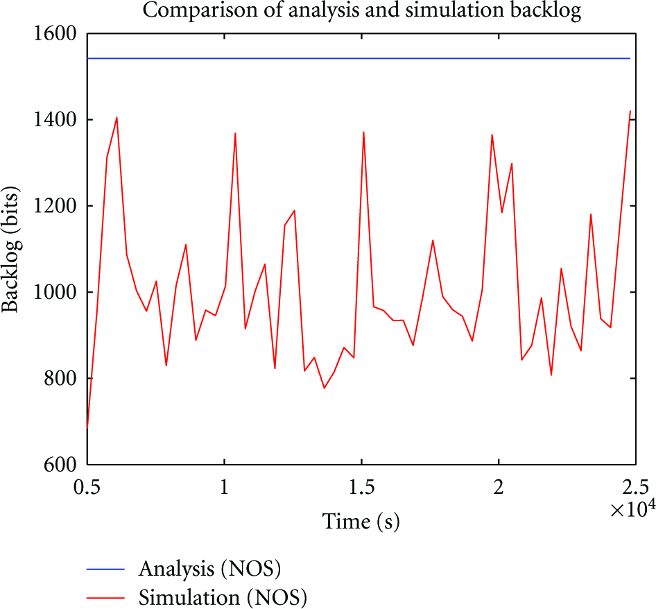
Nodes' backlogs in NOS.

Figure 24

Nodes' backlogs in FBS.

7. Conclusions and Future Work

Dimensioning timing-critical sensor networks requires formal methods to ensure performance and cost in any conditions. In this work, we present a network-calculus-based analysis method to compute the worst-case end-to-end delay bounds for individual flows, backlog bounds, and power consumptions for individual nodes. Based on network calculus and the splitting model, we are able to compute per-flow equivalent service curve provided by the tandem of visited nodes and the input and departure arrival curves of each node. Consequently, we can derive the performance bounds for the network which applies the flow-based traffic splitting strategy. Under the assumptions of affine arrival curve and rate-latency service curves, closed-form formulas of these bounds are computed. The numerical results for the example scenario show that, by applying the splitting strategy, the end-to-end delay can be reduced in most cases, the maximum backlog can be reduced up to 40%, and the power consumption can be reduced up to 15%. Furthermore, the simulation results verify that the theoretical bounds of our analysis are valid and fairly tight.

As stated in Section 4.4, there are several directions for future work. First, we will study the problem of designing a splitting scheme, this is, how to select splitting parameters based on network state information. Another research issue is to explore the optimized design space with given buffer sizes, performance requirements, and energy constraints for specific applications.