Numerical Simulation and Analysis of Gas-Liquid Flow in a T-Junction Microchannel

Abstract

Gas-liquid flow in microchannels is widely used in biomedicine, nanotech, sewage treatment, and so forth. Particularly, owing to the high qualities of the microbubbles and spheres produced in microchannels, it has a great potential to be used in ultrasound imaging and controlled drug release areas; therefore, gas-liquid flow in microchannels has been the focus in recent years. In this paper, numerical simulation of gas-liquid flows in a T-junction microchannel was carried out with computational fluid dynamics (CFD) software FLUENT and the Volume-of-Fluid (VOF) model. The distribution of velocity, pressure, and phase of fluid in the microchannel was obtained, the pressure distribution along the channel walls was analyzed in order to give a better understanding on the formation of microbubbles in the T-junction microchannel.

1. Introduction

Gas-liquid flow in microchannels is widely used in biomedicine, nanotech, sewage treatment, and so forth and has gained much interest in recent years. Gas-liquid two-phase flow in microchannels often exhibits different flow behavior than in macrosized conduits. Unlike the conventional channels, the surface tension in microchannels is dominant and the effect of gravity is almost negligible.

One of the common microfluidic devices is the T-junction reactor/mixer, which has a T-shaped microchannel etched on the substrate and a cover glass sealed the microchannel. It has become the most popular way to produce microbubbles and droplets in such channels [1]. Depending upon the geometries, properties and flow rates of the two fluids, various flow patterns, such as slug or Taylor, churn, rivulet, wavy annular, and annular flow, occur in gas-liquid flow in the T-junction microchannels [2]. Among different flow patterns in the T-junction microchannels, slug or Taylor flow is the most desired flow pattern for microbubble production, as it can generate microbubbles with high monodispersity. The mechanism of microbubble formations in the T-junction microchannels has been studied intensively in order to produce microbubbles in a controlled and reproducible manner.

Baround et al. [3] gave a detailed review on the effects of channel dimensions, viscosity, and flow rate ratio of the two immiscible fluids on the droplet formation. One of the explanations is that the slug or Taylor flow breaksup into separate bubbles owing to the pressure difference across the slug breaking neck, as the so-called squeezing effect [1]. At low capillary numbers (Ca < 10⁻²), the interfacial tension is strong compared to viscous stress, the droplets obstructs the channel as it grows, restricting the flow of continuous phase around it, stable parallel dispersed microbubbles are produced in this regime. At high capillary numbers, the droplets are emitted before they can block the channel and their formation is entirely due to the action of shear stress, this process is clarified as dripping regime. Indeed, the local flow field, which deforms the interface and eventually leads to the slug pinch off and form uniform microbubbles, may hold the key to the bubble formation mechanism [3]; therefore, more attention should be paid to the local flow filled near the breaking area.

The main objective of the present study is to perform numerical modeling of gas-liquid two-phase flow in a T-junction microchannel geometry, the velocity and pressure distribution along the channel and near the slug breaking area is also analyzed in order to obtain a comprehensive understanding of microbubble formation in the T-junction microchannels.

2. Mathematical Model and Numerical Algorithm

2.1. Governing Equations

The usual approach to the modeling of multiphase flow in microchannels is to compute the evolution of the gas-liquid interface [4]. In order to track the interface between the gas and liquid, one of the general multiphase models in FLUENT, the VOF model, is adopted to simulate gas-liquid flows in the T-junction microchannel. Among these multiphase models in the software FLUENT, such as VOF model, mixture model and Eulerian model, VOF model is the only model which can identify the interface clearly. The VOF model operates under the principle that two or more fluids are not interpenetrating. In the VOF model, different fluid phases are described by the same momentum equation, and the respective volume fraction of the phase is calculated in each computational cells.

The governing equations of the VOF formulations on multiphase flow are as follows.

Equation of continuity:

$\begin{array}{c}\frac{\partial \rho }{\partial t}+\nabla \cdot \left(\rho \overrightarrow{v}\right)=\mathrm{0};\end{array}$

1

equation of motion:

$\begin{array}{c}\frac{\partial }{\partial t}\left(\rho \overrightarrow{v}\right)+\nabla \cdot \left(\rho \overrightarrow{v}\overrightarrow{v}\right)=-\nabla \rho +\nabla \cdot \left[\mu \left(\nabla \overrightarrow{v}+\nabla {\overrightarrow{v}}^T\right)\right]+\overrightarrow{F};\end{array}$

2

volume fraction equation:

$\begin{array}{c}\frac{\partial {\Omega }_G}{\partial t}+\overrightarrow{v}\cdot \nabla {\Omega }_G=\mathrm{0},\end{array}$

3

where $\overrightarrow{v}$ is the velocity vector, ρ the density, μ the dynamic viscosity, $\overrightarrow{F}$ the surface tension force of the fluid, and ${\mathrm{\Omega }}_G$ the volume fraction of gas phase. The continuum surface force (CFS) model [5] was used to model the surface tension. The bulk properties such as density and viscosity are determined from the volume fraction weighed average of the properties of the two fluids, that is,

$\begin{array}{c}\rho ={\Omega }_G{\rho }_G+\left(\mathrm{1}-{\Omega }_G\right){\rho }_L,\hspace{1em}\hspace{1em}\mu ={\Omega }_G{\mu }_G+\left(\mathrm{1}-{\Omega }_G\right){\mu }_L,\end{array}$

4

where the subscript G indicates gas and L indicates the liquid phase.

In the present work, the flow field has been calculated using 2D and in some case, the calculation was performed in 3D geometry in order to save computational time and effort. A pressure-based unsteady solver was used along with the implicit body force formulation. PRESTO method was used for the pressure interpolation. PISO algorithm and second-order upwind scheme were used for the pressure-velocity coupling and momentum equations, respectively. Air was chosen as the primary phase and water as the second phase. The interface tension was set to 73.5 dyn/cm and the gas liquid wall contact angle was set to 36° [6]. The setup of the initial condition for the simulation is that the air and water inlets are set to the velocity inlet and the outlet is the pressure outlet.

2.2. Channel Geometry

Figure 1(a) shows the 2D rectangular T-junction microchannel dimension used in this study. The widths of the air inlet, water inlet and outlet are 118 μm, 111 μm, and 108 μm, respectively. The unit of the channel length is micrometer. The 3D geometry is shown in Figure 1(b), the depth of each channel is 119 μm.

Figure 1:

T-junction microchannel dimension used in the simulations. (a) 2D geometry; (b) 3D geometry.

At the initial stage, the main channel was filled with water and the side channel with air, and then the air and water were fed into the channel with a constant velocity. The flow was treated as laminar flow in the inlets. A quadrilateral paved grid was meshed and the grid independence was performed as shown in Figure 2. The air-water volume fraction plot for different grid elements sizes ranging from 11.1 μm to 2.77 μm in the T-junction microchannel was carried out. Both water and air velocity was set to 0.2 m/s. The air-water interface became sharp, and the air slug was independent of the grid size upon grid refinements. The interface is in a good accordance with the chosen contact angle of 36°. At the mesh sizes of 3.70 μm and 2.77 μm, the air slug disappeared and stratified flow was observed, which is in a good agreement with the experimental observations by Santos and Kawaji [6]. It indicates that the grid independence was achieved. However, the ultrafined grids are not necessary since they are usually computationally expensive. Therefore, the mesh with element size of 3.70 μm was finally chosen in this study.

Figure 2:

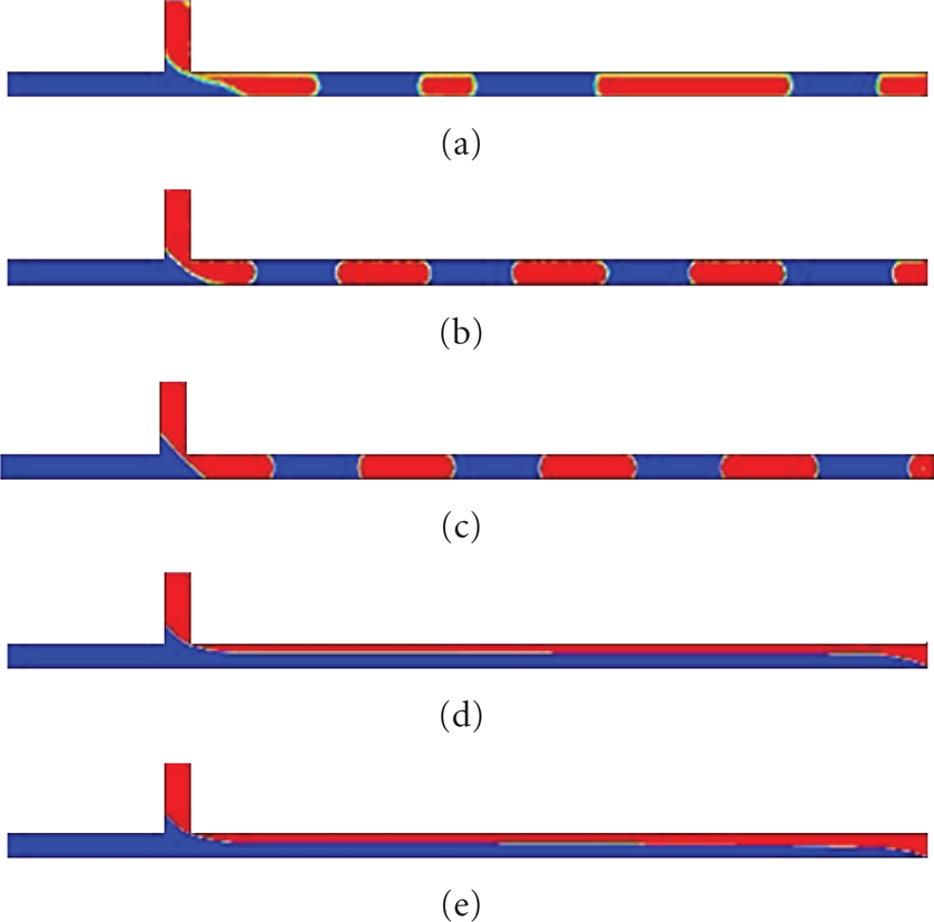
Plots of air-water volume fraction for different meshes. The air is colored in red and the water is colored in blue. (a) element size 11.10 μm; (b) element size 7.40 μm; (c) element size 5.67 μm; (d) element size 3.70 μm; (e) element size 2.77 μm.

3. Results and Discussion

A set of simulations was performed with the superficial velocities of the air and water ranging from 0.01 m/s to 0.90 m/s. Capillary number (Ca) is calculated as $\text{Ca}={\mu }_c{U}_c/\gamma$ , where μ _c , U _c , and γ are the average inlet velocity of the continuous phase, the dynamic viscosity of the continuous phase, and the interfacial tension between the two phases, respectively.

3.1. Different Flow Patterns

In the experimental study of Santos and Kawaji [6], two types of flow patterns were observed: slug flow and stratified flow. Furthermore, during the slug flow, it was observed that the slugs were produced in three different manners in the T-junction, and the patterns were referred to as breaking slug, snapping slug, and jetting slug.

(1) Stratified Flow Pattern

As the gas and liquid velocity set to U _G = 0.237 m/s and U _L = 0.252 m/s, respectively, the flow exhibits a stratified pattern as shown in Figure 3(b) and it is in a good agreement with the experimental results as shown in Figure 3(a). The $\text{Ca}=\mathrm{3}.\mathrm{35}\times \mathrm{1}{\mathrm{0}}^{-\mathrm{3}}$ , the ratio of the gas liquid flow rates ∊ = UG/U _L is 0.94, there are no bubbles formed, the air flow did not form a thin neck around the T joint; therefore, no breaking occurred.

Figure 3:

Stratified flow (U _G = 0.237 m/s; U _L = 0.252 m/s). (a) experimental results [6]; (b) numerical simulation.

(2) Slug Flow

By changing the ratio of the gas liquid velocities ε, the flow pattern changed from the stratified flow to the slug flow. The snapping slug formation, breaking slug formation, and jetting slug formation are shown in Figures 4, 5 and 6, respectively.

Figure 4:

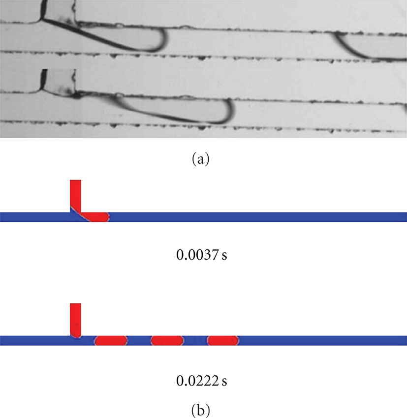
Snapping slug formation (U _G = 0.158 m/s; U _L = 0.042 m/s). (a) experimental results [6]; (b) Numerical simulation.

Figure 5:

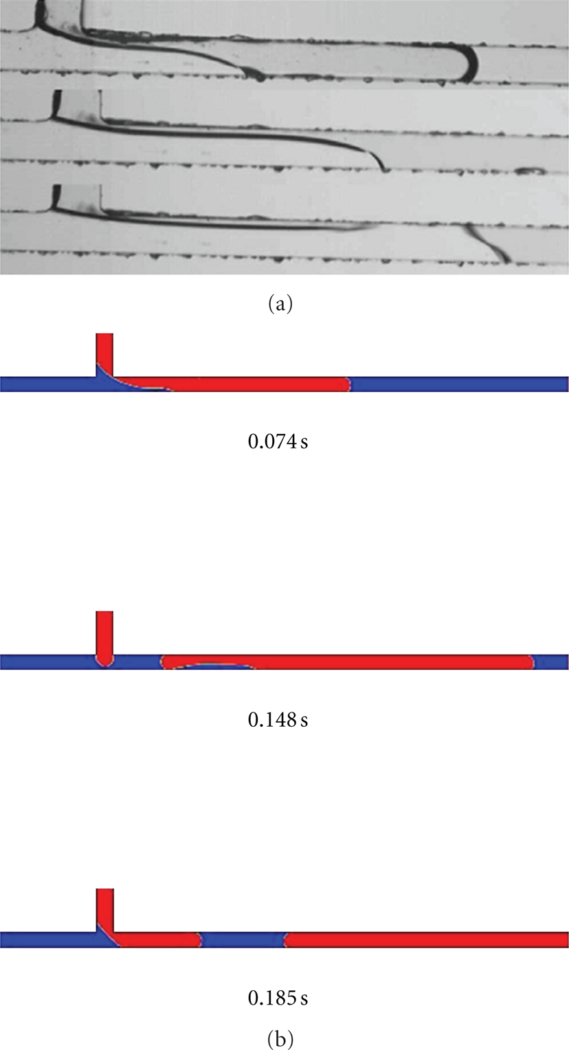
Breaking slug formation (U _G = 0.317 m/s; U _L =; U _L = 0.336 m/s). (a) experimental results [6]; (b) numerical simulation.

Figure 6:

Jetting slug formation (U _G = 0.435 m/s; U _L = 0.757 m/s). (a) experimental results [6]; (b) numerical simulation.

At $\text{Ca}=\mathrm{5}.\mathrm{60}\times \mathrm{1}{\mathrm{0}}^{-\mathrm{4}}$ , a higher gas liquid flow rate ratio ε = 3.7 as observed in the experimental study [6] of the snapping slug formation (shown in Figure 4(a)), the gas slug touches both the top and bottom channel wall while it is still growing. The slug blocks the entire channel and moves toward the downstream by the push of the liquid stream and propagation of the gas bulk. Once the tail thins, it snaps at the top wall creating a fourth contact point. The interfacial tension could contribute to the thinner of the slug thread; therefore, the snapping slug pattern could be classified into the squeezing regime. The numerical simulation forms a long gas slug which matches the experiment results.

In the breaking slug formation (as shown in Figure 5(a), $\text{Ca}=\mathrm{4}.\mathrm{48}\times \mathrm{1}{\mathrm{0}}^{-\mathrm{3}},\epsilon =\mathrm{0.94}$ ), the gas slug flows toward the top channel wall forming a contact point. The liquid stream pushes the air-water interface forward and some liquid flows underneath the gas slug. Santos and Kawaji [6] explained that the gas bulk will neck and then break off when the surface tension cannot hold the slug connected to the air inlet. The numerical simulation was carried out in 3D geometry. In the numerical simulation at 0.0222 s (shown in Figure 5(b)), the slug breaks off at the T joint, then being pushed forward. With the increase of gas velocity, the slug size is smaller compared with the snapping slug formation regime as shown in Figure 4(a).

In the experimental results of the jetting slug formation (Figure 6), Ca =1.01×10⁻², the gas flow rate is higher than the breaking and snapping slug flow, the gas liquid ratio ε = 0.57, the gas stream protrudes into the main channel and gas slugs pinch off with the propagation of gas bulk in a regular interval. The numerical simulation was carried out in 3D geometry, the results were in a good agreement with the experimental observations [6]. The gas slug breaks into separate microbubbles in the main stream, while being pushed forward by the liquid stream, which is different from the breaking and snapping slug formation.

The flow patterns were correlated with the inlet velocities to produce an experimental flow pattern map, as shown in Figure 7. The experimental results show that the snapping regime is dominant at low liquid superficial velocities. The flow pattern transforms to breaking slug with the rising liquid superficial velocity. When the gas superficial velocity is high, the breaking slug usually alternates with stratified flow. The jetting regime only exists when both gas and liquid velocities are high as shown in Figure 7(a).

Figure 7:

T-junction experimental flow pattern map. (a) experimental results [6]; (b) numerical simulation.

Figure 7(b) shows the numerical simulations of flow pattern map with about 27 simulation runs. Flow patterns are defined with the number of the interface contact points during the slug formation. The contact points of breaking, snapping, and jetting are 1, 3, and 0, respectively. Given the inaccuracy of the stratified flow prediction, the numerical flow pattern map was simplified without the stratified flow. But the trend of pattern transition matches the experimental results. With the increasing of gas superficial velocities and same gas superficial velocity, the gas-liquid phase flow pattern transforms from snapping regime to breaking regime. The jetting regime only exists when the gas and liquid velocities are both high, which is in a good agreement with experimental observations. Both numerical and experimental studies showed that in the Ca range of 10⁻⁴–10⁻², the gas flow rate could be the dominant factor for the slug formation and size.

3.2. Analysis of Gas Liquid Flow in a T-Junction Microchannel

According to the numerical research of Guo and Chen [7], the velocity distribution at the mixing zone has two different regimes (squeezing regime and shearing regime). In the squeezing regime, the main flow direction of the liquid phase is perpendicular to the gas-liquid interface and the liquid phase pushes the interface toward the corner of the wall and the interface will break at the sharp corner (the T joint). In the shearing regime, the main direction of the liquid phase is along the interface and the interface will break off in the main stream near the upper wall.

The velocity distribution of the jetting slug formation at the gas liquid mixing zone is presented in Figure 8. It can be seen that the main direction of liquid phase is along the interface, so its flow is in shearing regime. It eventually breaks into separate microbubbles as shown in Figure 6(b). Therefore when Ca > 10⁻², the viscous stress is strong, the formation of the microbubbles is due to the shearing effect, the gas slug did not break off at the T joint.

Figure 8:

Distribution of the jetting mixing zone (U _G = 0.435 m/s; U _L = 0.757 m/s). (a) volume fraction distribution; (b) velocity distribution.

The numerical simulation shows that the snapping slug formation can be classified as in the squeezing regime, shown in Figure 9. Two vortexes near the slug breaking point were found. Their interfaces break at the sharp corner of the mixing zone. The main flow direction of the liquid phase is perpendicular to the gas-liquid interface, and the liquid phase pushes the interface toward the corner of the wall and the interface will break at the sharp corner. Therefore, the squeezing effect could contribute to the slug breaking off. Gas vortex was also found in the slug after the breaking off. The vortex formation could be the reason to induce the slug breaking off. A similar result was also found for the breaking slug formation.

Figure 9:

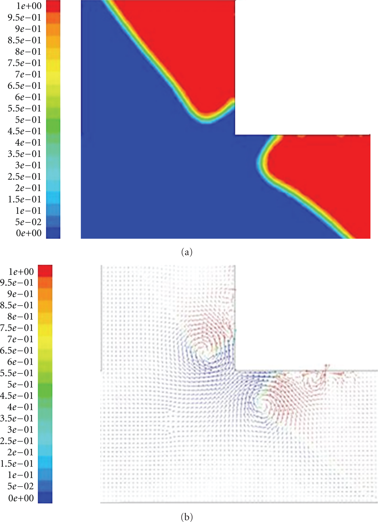
Velocity distribution at the snapping mixing zone (U _G = 0.110 m/s; U _L = 0.018 m/s). (a) the gas-liquid phase; (b) velocity distribution.

3.3. Pressure Distribution

Figure 10 shows the pressure distribution in the jetting slug flow. As the viscosity ratio of the two immiscible liquids is ≫1, there is no pressure drop in the slug as shown in Figure 10(b), which is also predicted by Baroud et al. [3]. The pressure drop can be useful to determine the size of the microbubbles and the frequency. The pressure in the liquid stream and the gas slug is different due to the existence of Laplace pressure and dynamic head. The pressure profile on the axis as shown in Figure 10(b) is similar to the pressure profile from Qian and Lawal [8]. It can be seen that the pressure drop across the back interface is higher than that across the front interface. The pressure distribution along the top and bottom wall exhibits the same profile as along the axis. The same phenomena of pressure distribution as above were observed in the snapping slug flow simulation as well.

Figure 10:

Pressure distribution of the jetting slug formation. (a) phase contour for the jetting slug formation; (b) pressure profile.

4. Conclusions

In this paper, the flow patterns of gas-liquid flow in a T-junction microchannel was numerically studied with the VOF model using FLUENT software. A numerical flow pattern map were drawn to compare with the experimental results. When the Ca is higher than 10⁻², the jetting slug formation was observed and it falls into the shearing regime, in which the viscous stress is strong compared to the interfacial tension. At lower Ca numbers, the gas flow rate could be the dominant factor for the slug formation and size.

The velocity distribution and pressure profile along the channel walls were studied. Two vortexes were found near the slug breaking point, and pressure drops were observed in the numerical simulation. It could be the main reason for the slug breaking into bubbles. The breaking and snapping slug formation is in the squeezing regime, while the jetting slug formation falls into the shearing regime.