Improved DV-Hop Node Localization Algorithm in Wireless Sensor Networks

Abstract

An improved algorithm is put forward to improve the poor locating performance of the DV-Hop algorithm, which is one of the range-free algorithms in wireless sensor networks. Firstly, we set some anchor nodes at the border land of monitoring regions. Secondly, the average one-hop distance between anchor nodes is modified, and the average one-hop distance used by each unknown node for estimating its location is modified through weighting the received average one-hop distances from anchor nodes. Finally, we use the particle swarm optimization to correct the position estimated by the 2D hyperbolic localization algorithm, which makes the result closer to the actual position. The simulation results show that the proposed algorithm has better localization performance in the localization precision and stability than the basic DV-Hop algorithm and some existing improved algorithms.

1. Introduction

Wireless sensor networks (WSNs) are composed of plenty of sensor nodes that are deployed in the monitoring field, and they form a multihop self-configured network by means of wireless communication. The sensor nodes have perception, processing, and communication ability [1].

In many applications of WSNs, the monitoring data is of no significance if the locations of sensors are unknown because the position is needed to locate events that occurred in WSNs. Positioning information can be used not only to report events place, but also for the target tracking, the target track prediction, the assist routing and the topology of the network management, and so forth.

On the basis of whether it is required to measure the actual distances between nodes, the nodes localization algorithms can be classified into two categories, that is, range-based and range-free [2]. The former exploits the distance or angle information between neighbor nodes and then uses the trilateral or multilateral localization methods to locate the unknown nodes, such as RSSI [3], TDOA [4], TOA [5], and AOA [6]. The latter uses the estimated distance instead of the metrical distance to locate the unknown nodes, such as the centroid algorithm [7], the DV-Hop algorithm and the convex programming algorithm [8]. Due to the high cost of hardware facilities and energy consumption required by range-based approaches, the range-free algorithms attract more and more attention.

In this paper, we present an improved DV-Hop algorithm, which can reduce the localization error. At first few anchor nodes are properly distributed. The average hop distance is calculated in a different way, in which not only the global property of average hop size and anchor nodes are considered. Finally, the particle swarm optimization algorithm is used to correct the position estimated by the 2D hyperbolic location algorithm. The rest of the paper is organized as follows. Section 2 describes the basic DV-Hop algorithm and some existing improved DV-Hop algorithms. In Section 3, we propose the modified DV-Hop algorithm. In Section 4, simulation results are presented and analyzed. Section 5 analyses communication cost and computational efficiency. Finally, we conclude the paper in Section 6.

2. Related Works

2.1. DV-Hop Localization Algorithm

DV-Hop (distance vector-hop) localization algorithm [9], which was proposed by Dragos Niculescu, is one of the typical representatives of range-free localization algorithm. Its basic idea is that the distance between the unknown nodes and the reference nodes is expressed by the product of average hop distance and the hop count.

The algorithm implementation is comprised of three steps. In the first step, each anchor node broadcasts an anchor to be flooded throughout the network containing the anchors location with a hop count value initialized to one. Each receiving node maintains the minimum hop count value. Anchors with higher hop count values to a particular anchor are defined as the useless information and ignored. Then, rest of the anchors are flooded outward with hop count values incremented at every intermediate hop. Through this process, all nodes in the network get the minimal hop count to every anchor node.

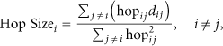
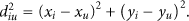
In the second step, once an anchor gets hop count value to other anchors, it estimates an average size of one hop, which is then flooded to the entire network. After receiving the hop size, the unknown nodes multiply the hop size by the hop count value to derive the estimated physical distance from the anchor. The average hop size is estimated by the anchor node i using the following formula:

$$\begin{array}{cc}& {\text{Hop}\mathrm{\hspace{0.17em}\hspace{0.17em}}\text{Size}}_i=\frac{{\sum }_{j\ne i}\sqrt{{\left(x_i-x_j\right)}^{\mathrm{2}}+{\left(y_i-y_j\right)}^{\mathrm{2}}}}{{\sum }_{j\ne i}{\text{hop}}_{ij}},\end{array}$$

(1)

where ( $x_i$ , $y_i$ ) and ( $x_j$ , $y_j$ ) are coordinates of anchor nodes i and j, respectively, and ${\text{hop}}_{ij}$ is the hop count between the anchor nodes i and j.

Each anchor node broadcasts its hop size to the network using controlled flooding. Unknown nodes receive the hop size information and save the first one. Meanwhile, they transmit the hop size to their neighbor nodes. This scheme ensures that most nodes receive the hop size from the anchor node that has the least hops between them.

In the last step, when unknown nodes get three or more distance information from anchor nodes, the trilateral measuring method or the maximum likelihood estimation method is used to calculate their locations.

It is assumed that ( $x_u,y_u$ ) are the location of the unknown node u and ( $x_i,y_i$ ) are the known location of the ith anchor node. $d_{ui}$ is the distance between them. Then, we have

$$\begin{array}{cc}& {\left(x_u-x_{\mathrm{1}}\right)}^{\mathrm{2}}+{\left(y_u-y_{\mathrm{1}}\right)}^{\mathrm{2}}=d_{u\mathrm{1}}^{\mathrm{2}}\\ {\left(x_u-x_{\mathrm{2}}\right)}^{\mathrm{2}}+{\left(y_u-y_{\mathrm{2}}\right)}^{\mathrm{2}}=d_{u\mathrm{2}}^{\mathrm{2}}\\ ⋮\\ {\left(x_u-x_n\right)}^{\mathrm{2}}+{\left(y_u-y_n\right)}^{\mathrm{2}}=d_{un}^{\mathrm{2}}.\end{array}$$

(2)

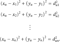
The coordinates of u are computed by the following formula:

$$\begin{array}{cc}& A=-\mathrm{2}\times \left[\begin{array}{cc}{x}_{\mathrm{1}}-x_n& y_{\mathrm{1}}-y_n\\ x_{\mathrm{2}}-x_n& y_{\mathrm{2}}-y_n\\ ⋮& ⋮\\ x_{n-\mathrm{1}}-x_n& y_{n-\mathrm{1}}-y_n\end{array}\right],\end{array}$$

(3)

$$\begin{array}{cc}& B=\left[\begin{array}{c}{d}_{u\mathrm{1}}^{\mathrm{2}}-d_{un}^{\mathrm{2}}-x_{\mathrm{1}}^{\mathrm{2}}+x_n^{\mathrm{2}}-y_{\mathrm{1}}^{\mathrm{2}}+y_n^{\mathrm{2}}\\ d_{u\mathrm{2}}^{\mathrm{2}}-d_{un}^{\mathrm{2}}-x_{\mathrm{2}}^{\mathrm{2}}+x_n^{\mathrm{2}}-y_{\mathrm{2}}^{\mathrm{2}}+y_n^{\mathrm{2}}\\ ⋮\\ d_{u(n-\mathrm{1})}^{\mathrm{2}}-d_{un}^{\mathrm{2}}-x_{n-\mathrm{1}}^{\mathrm{2}}+x_n^{\mathrm{2}}-y_{n-\mathrm{1}}^{\mathrm{2}}+y_n^{\mathrm{2}}\end{array}\right],\end{array}$$

(4)

$$\begin{array}{cc}& P=\left[\begin{array}{c}{x}_u\\ y_u\end{array}\right],\end{array}$$

(5)

and $P=(A^{T}A{)}^{-\mathrm{1}}{A}^{T}B$ .

2.2. Existing Improved DV-Hop Algorithms

When the nodes are uniform and isotropic in WSNs, it is reasonable to get every average hop distance so that the positioning accuracy is proper. But when the network is sparse or nodes are distributed unevenly, nodes often receive inaccurate hop information and calculate the every average hop distance with bigger errors, which affects the network node location accuracy.

To solve this, many scholars improved the DV-Hop algorithm from all aspects. Zhang fixed the anchor nodes at the border land of the network, which saved the number of anchor nodes [10]. Shi used the cluster strategy to reduce the communication cost and group the conflict probability in the first stage and used the quasi-Newton optimization algorithm to estimate the position of nodes, which improved the localization accuracy without increasing communications traffic [11]. Gao et al. formulated the hop-distance relationship for the quasi-UDG model in WSNs [12]. They derived an approximated recursive expression for the probability of the hop count with a given geographic distance. The border effect and dependence problem are also taken into consideration. Furthermore, they gave expressions describing the distribution of distance with known hop counts for inner nodes and those suffering from the border effect. Lee proposed a novel localization scheme based on the DV-Hop algorithm to improve the positioning accuracy with the least error hop sizes of anchors and average hop sizes of unknowns, each unknown node calculated its average hop size with hop sizes from anchors [13]. Lin put forward three approaches to improve the poor locating performance [14]. Firstly, the average one-hop distance between anchor nodes was refined by means of the least square method. Secondly, the average one-hop distance was modified through weighting the received average one-hop distances from anchor nodes. Finally, the iterative numerical method with the initial values of the estimated node location was presented by setting proper threshold. Shi corrected the average hop distance of anchor nodes by the total error between the calculated distances and the estimated distances and used 2D hyperbolic location algorithm, which improved the localization accuracy effectively [15]. Sezaki used a differential error correction scheme designed to reduce the location error accumulated over multiple hops [16]. Gao put forward a WSN localization algorithm based on the adaptive particle swarm optimization [17].

3. Improved DV-Hop Algorithm

In this paper, we propose an improved DV-Hop algorithm, which is divided into the following four steps. (1) Some anchor nodes are fixed at the border land of the monitoring regions. (2) The average one-hop distance among anchor nodes is modified, and the average one-hop distance used by each unknown node for estimating its location is modified. (3) The unknown nodes’ positions are obtained by the 2D hyperbolic location algorithm. (4) We use the particle swarm optimization algorithm to correct the estimated position.

3.1. Deploy Anchor Nodes

Because anchor nodes are randomly distributed in DV-Hop algorithm, some anchor nodes may concentrate in an area. If we use those anchor nodes to estimate unknown nodes positions, it will produce larger error and bad stability unless the network has high similarity. Therefore, we fix some anchor nodes at the borderland of the monitoring regions firstly, and the rest of the anchor nodes are distributed randomly [10].

3.2. Calculation of the Average Hop Distance of Unknown Nodes

We modify the network average hop distance to improve the localization accuracy. The average hop distance of every anchor node $\text{Hop}\mathrm{\hspace{0.17em}\hspace{0.17em}}{\text{Size}}_i$ is revised based on the least square error criterion mentioned previously [14]:

$$\begin{array}{cc}& {\text{Hop}\mathrm{\hspace{0.17em}\hspace{0.17em}}\text{Size}}_i=\frac{{\sum }_{j\ne i}\left({\text{hop}}_{ij}{d}_{ij}\right)}{{\sum }_{j\ne i}{\text{hop}}_{ij}^{\mathrm{2}}},\hspace{1em}i\ne j,\end{array}$$

(6)

where $d_{ij}$ is the straight-line distance between the anchor nodes i and j.

Then, we modify the average one-hop distance of unknown nodes ${\text{Hop}\mathrm{\hspace{0.17em}\hspace{0.17em}}\text{Size}}_u$ through weighting the N received average one-hop distances from the anchor nodes by the following formula:

$$\begin{array}{cc}& {\text{Hop}\mathrm{\hspace{0.17em}\hspace{0.17em}}\text{Siz}e}_u={\sum }_{i=\mathrm{1}}^n{\lambda }_i\hspace{0.17em}{\text{Hop}\mathrm{\hspace{0.17em}\hspace{0.17em}}\text{Size}}_i,\\ {\lambda }_i=\frac{{\text{hop}}_i}{{\sum }_{k=\mathrm{1}}^n{\text{hop}}_k},\end{array}$$

(7)

where ${\text{hop}}_i$ is the hop segment number between the unknown node u and the anchor node i in its routing table and n is the number of all anchor nodes.

The total of weighting value of all anchor nodes in the routing table of unknown node is 1. By the weighted average, the average hop distance of unknown nodes is reflected from the one-hop distance of all anchor nodes.

3.3. Position Determination of Unknown Nodes

We use the 2-D Hyperbolic location algorithm instead of the traditional trilateral or the multilateral position method to estimate the position of unknown nodes, which improves the estimated location precision.

It is assumed that ( $x_i,y_i$ ) are the coordinates of anchor node i and ( $x_u,y_u$ ) are the coordinates of unknown node u. The estimated distance $d_{iu}$ between them is

$$\begin{array}{cc}& d_{iu}^{\mathrm{2}}={\left(x_i-x_u\right)}^{\mathrm{2}}+{\left(y_i-y_u\right)}^{\mathrm{2}}.\end{array}$$

(8)

If $A_i=x_i^{\mathrm{2}}+y_i^{\mathrm{2}}$ and $B_u=x_u^{\mathrm{2}}+y_u^{\mathrm{2}}$ , (4) takes the form

$$\begin{array}{cc}& d_{iu}^{\mathrm{2}}-A_i=-\mathrm{2}{x}_i{x}_u-\mathrm{2}{y}_i{y}_u+B_u.\end{array}$$

(9)

Equation (9) in the matrix form is

$$\begin{array}{cc}& GZ=h,\end{array}$$

(10)

where

$$\begin{array}{cc}& Z={\left[x_u,y_u,B_u\right]}^T,\hspace{1em}\hspace{1em}G=\left[\begin{array}{ccc}-\mathrm{2}{x}_{\mathrm{1}}& -\mathrm{2}{y}_{\mathrm{1}}& \mathrm{1}\\ -\mathrm{2}{x}_{\mathrm{2}}& -\mathrm{2}{y}_{\mathrm{2}}& \mathrm{1}\\ ⋮& ⋮& ⋮\\ ⋮& ⋮& ⋮\\ -\mathrm{2}{x}_n& -\mathrm{2}{y}_n& \mathrm{1}\end{array}\right],\\ h=\left[\begin{array}{c}{d}_{\mathrm{1}u}^{\mathrm{2}}-A_{\mathrm{1}}\\ d_{\mathrm{2}u}^{\mathrm{2}}-A_{\mathrm{2}}\\ ⋮\\ ⋮\\ d_{nu}^{\mathrm{2}}-A_n\end{array}\right].\end{array}$$

(11)

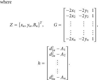
According to (10), Z can be obtained by using the least mean square estimation method:

$$\begin{array}{cc}& Z={\left(G^{T}G\right)}^{-\mathrm{1}}{G}^{T}h.\end{array}$$

(12)

Therefore, the coordinates of unknown node u are

$$\begin{array}{l}{x}_u=Z\left(\mathrm{1}\right),\\ y_u=Z\left(\mathrm{2}\right).\end{array}$$

(13)

3.4. Particle Swarm Optimization

The particle swarm optimization (PSO) [18], one branch of heuristic methods, is especially useful in dynamically changing domains. PSO algorithm initializes a set of random solutions for the objective function and takes each individual solution as one particle. Each particle has an objective function determined by the fitness value, and it also has a rate determined by the distance and direction of particle search. We can determine the pros and cons of the particle based on the fitness value. According the two extremes, the individual extreme (p best) is the optimal position of the current search of the particle and the global minimum (g best) is the optimal position of the current search of all group particles. Each particle can update its velocity and position by

$$\begin{array}{l}{v}_u^{k+\mathrm{1}}={\omega v}_u^k+c_{\mathrm{1}}\hspace{0.17em}{\text{rand}}_{\mathrm{1}}^k\left({p\hspace{0.17em}\text{best}}_u^k-X_u^k\right)\\ +c_{\mathrm{2}}\hspace{0.17em}{\text{rand}}_{\mathrm{2}}^k\left(g\hspace{0.17em}\text{bes}{\text{t}}^k-X_u^k\right),\\ X_u^{k+\mathrm{1}}=X_u^k+v_u^{k+\mathrm{1}},\end{array}$$

(14)

where $v_u^k$ is the velocity vector, $X_u^k$ is the current position vector of the particle and its initial value is obtained by using (13), ${p\hspace{0.17em}\text{best}}_u^k$ is the individual extreme of the particle u by k-cycles, and ${g\hspace{0.17em}\text{best}}_u^k$ is the global extreme of all particles by k-cycles. In the typical PSO implementation, $c_{\mathrm{1}}$ and $c_{\mathrm{2}}$ are the acceleration factors and ${\text{rand}}_{\mathrm{1}}^k$ and ${\text{rand}}_{\mathrm{2}}^k$ are both random of $[0,1]$ . k is the current number of iterations.

The inertia weight, ω, is used to maintain the global and local search for the balance. The value of ω needs to be set large to jump out of the local minimum on the contrary to be set smaller to the convergence algorithm. In consideration of the global search, it is better to set large value for ω in the beginning while a small value for ω at the last stage. We take ω as the function of iterations which can linearly decrease by iterations

$$\begin{array}{cc}& \omega ={\omega }_{\max }-\frac{{\omega }_{\max }-{\omega }_{\min }}{{\text{iter}}_{\max }}\times k,\end{array}$$

(15)

where ${\omega }_{\max \hspace{0.17em}}$ and ${\omega }_{\min \hspace{0.17em}}$ are the initial inertia weight and the termination inertia weight, respectively, ${\text{iter}}_{\max \hspace{0.17em}}$ is the maximum number of iterations, and k is the current number of iterations.

The fitness in our paper is designed as

$$\begin{array}{cc}& \text{fitness}\left(X_u\right)={\sum }_{i=\mathrm{1}}^n{\alpha }_i^{\mathrm{2}}{\left(d_i-\left|X_u-A_i^T\right|\right)}^{\mathrm{2}},\end{array}$$

(16)

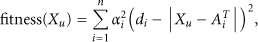
where $A_i^T$ is the position of the anchor node and ${\alpha }_i$ is inversely proportional to the hop count between the unknown node u and the anchor node i.

4. Simulation Results and Discussion

To evaluate the performance of our proposed algorithm, we use Matlab2009a as the simulator to implement the network scenario and determine the localization results. The simulation experiment environment is set as follows. Firstly four anchor nodes are fixed at the vertex of the sensor field of 100*100 m², and then unknown nodes and the rest of anchor nodes are distributed randomly.

The parameters in the PSO algorithm are $c_{\mathrm{1}}=c_{\mathrm{2}}=\mathrm{2.05}$ , ${\omega }_{\max \hspace{0.17em}}=\mathrm{0.9}$ , ${\omega }_{\min \hspace{0.17em}}=\mathrm{0.4}$ , ${\text{iter}}_{\max \hspace{0.17em}}=\mathrm{20}$ , the number of particles is 20, and $V_{\max \hspace{0.17em}}=\mathrm{10}\hspace{0.17em}\text{m}$ , which have been tested and verified by researchers before [18]. The network environment parameters of every simulation, such as the network area, the number of anchor nodes, the number of unknown nodes, and the radio range of sensor nodes, are the same. The algorithm localization accuracy and stability are, respectively, evaluated by the localization error and localization error variance, which are shown by

$$\begin{array}{l}\text{Average}\mathrm{\hspace{0.17em}\hspace{0.17em}}\text{Error}=\frac{{\sum }_{k=\mathrm{1}}^n\left|{\widehat{X}}_u-X_u\right|}{n\times R},\\ \text{Localization}\mathrm{\hspace{0.17em}\hspace{0.17em}}\text{Error}\mathrm{\hspace{0.17em}\hspace{0.17em}}\text{Variance}\\ \hspace{1em}\hspace{1em}\hspace{1em}\hspace{1em}\hspace{1em}=\sqrt{\frac{{{\sum }_{i=\mathrm{1}}^n\left(\left|{\widehat{X}}_u-X_u\right|-\text{Average}\mathrm{\hspace{0.17em}\hspace{0.17em}}\text{Error}\times R\right)}^{\mathrm{2}}}{n\times R^{\mathrm{2}}}},\end{array}$$

(17)

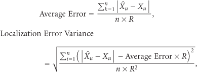
where n is the number of unknown nodes, $X_u$ is the unknown node u evaluated position, ${\widehat{X}}_u$ is the unknown node u actual position, and R is the radio range of sensor nodes.

The result data is the average of 100 experiments.

The localization error and error variance with different numbers of anchor nodes are shown in Figures 1 and 2. It is clear that the proposed algorithm is obviously better than the basic DV-Hop algorithm and the improved algorithm in the [14]. The localization error in our algorithm is about 13% lower than that in the basic DV-Hop algorithm and about 7% lower than that of [14]. Localization error variance decreases by about 7% and 3% correspondingly. The use of the PSO algorithm has fastened convergence speed apparently (the number of sensor nodes is set to 200 and R is set to 22 m).

Figure 1

Localization error with different number of anchor nodes.

Figure 2

Localization error variance with different number of anchor nodes.

The localization error and error variance with different numbers of sensor nodes are shown in Figures 3 and 4. It is shown that our proposed algorithm is obviously better than the basic DV-Hop algorithm and the improved algorithm in [14]. The localization error in our algorithm is about 14% lower than that in the basic DV-Hop algorithm and about 8% lower than that of [14]. Localization error variance decreases by about 6% and 3% correspondingly (the proportion of anchor nodes is set to 10% and R is set to 22 m).

Figure 3

Localization error with different number of sensor nodes.

Figure 4

Localization error variance with different number of sensor nodes.

The localization error and error variance with different radio ranges of sensor nodes are shown in Figures 5 and 6. It is clear that our improved algorithm is obviously superior to the basic DV-Hop algorithm and the improved algorithm proposed in [14]. The localization error in our algorithm is about 11% lower than that in the basic DV-Hop algorithm and about 6% lower than that of [14]. Localization error variance decreases by about 5% and 2% correspondingly (the number of sensor nodes is set to 200 and the proportion of anchor nodes is set to 10%).

Figure 5

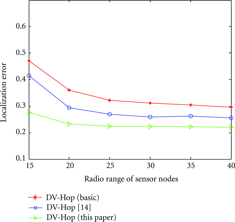
Localization error with different radio ranges of sensor nodes.

Figure 6

Localization error variance with different radio ranges of sensor nodes.

5. Communication Cost and Computational Efficiency

The algorithm communication cost is presented by the number of transmitting packets in process of localization. In this paper, we refine the average one-hop distance between anchor nodes and modify the average one-hop distance used by each unknown node for estimating its own location through weighting N received average one-hop distances from anchor nodes, and the date is saved by unknown nodes in the basic DV-Hop algorithm. So we do not need the extra communication cost.

The process used by the PSO algorithm for correcting the position estimates computed by the 2D hyperbolic location algorithm increases the computation time. Figure 7 shows the localization time comparison. The proposed algorithm is slower about 0.01 second than the original algorithm; meanwhile localization precision is improved. Therefore, we need to keep balance between the precision and the calculation in the practical application.

Figure 7

Localization time with different numbers of anchor nodes.

6. Conclusions

We have presented a modified DV-Hop localization algorithm to improve the poor locating performance of the DV-Hop algorithm, mainly focusing on the following steps. Firstly, some anchor nodes are distributed at the border land of the monitoring regions. Secondly, the average one-hop distance of anchor nodes is modified. Moreover, the average one-hop distance, which is used by each unknown node for estimating its own location, is modified by weighting N received average one-hop distances from anchor nodes. Finally, we use the PSO algorithm to correct the position estimated by the 2D hyperbolic location algorithm. It is shown that our proposed algorithm obviously improves the localization precision and stability. But it has very little increase in the computation time with respect to PSO.