A Mathematical Model for the Analysis of Elastic Field in a Stiffened Cantilever of Laminated Composite

Abstract

A mathematical model is developed for the analytical solution to elastic filed in a deep stiffened cantilever beam of laminated composite under mixed boundary conditions. The two displacement parameters associated with the two-dimensional elasticity problems are defined in terms of a single displacement potential function such that one of the equilibrium equations is satisfied automatically. This reduces the problem to the solution of a single fourth-order partial differential equation, which is solved in terms of Fourier series. To present some numerical results, cantilever beams of glass/epoxy cross-ply and angle-ply laminated composites are considered and different components of stress and displacement at different sections of the beam are presented. The effects of laminate stacking sequence and ply-angle of the cross-ply and angle-ply composite beams, respectively, on the elastic field are analyzed. The numerical results justify that the present mathematical model is simple whereas capable to generate exact results of elastic field in a cantilever beam even at the critical regions of supports and loadings.

1. Introduction

It is now well known that composite materials are superior to conventional monolithic materials in many respects. In particular, these materials possess superior mechanical properties, such as specific strength and stiffness, superior physical property, such as specific density, and superior thermal property, such as minimized coefficient of thermal expansion. As a result, these materials are being widely used in modern structural elements to ensure better characteristics. However, prior to their applications, these structural elements should be properly studied under actual boundary conditions in order to understand, quantify, and improve their characteristics. The elastic characteristic is one of such important issues that should be paid attention to understand the stress and displacement fields. In most of the cases, the boundary conditions experienced by engineering structural elements are of the mixed type. Thus, it is imperative to develop a suitable mathematical model that is capable of dealing with mixed boundary conditions as well as other boundary conditions. Obviously, experimental approaches are sometimes not feasible for complex boundary conditions and complex geometries of elements, in addition to the cost involved with experiments. Numerical approaches, on the other hand, are not always adequate to generate accurate results, particularly at and near the boundaries of structural elements. In an attempt to get rid of these problems, the present study is aimed to develop an analytical approach for the analysis of elastic field in a cantilever beam of laminated composite materials.

Airy stress function approach [1] appears to be convenient to obtain analytical solution only for some idealized two-dimensional elasticity problems when boundary conditions are prescribed in terms of stresses only. It appears to be inadequate for the problems when the boundary conditions are prescribed in terms of displacement or strain. Displacement parameter approach [2] formulates the two-dimensional elasticity problems in terms of two displacement parameters u _x and u _y . Thus, this approach can be used for the solution of problems associated with displacement boundary conditions. However, this approach involves two major difficulties. Firstly, formulations of two-dimensional elasticity problems in terms of displacement parameters yield two simultaneous second-order partial differential equations which are quite difficult to solve analytically. Secondly, the mixed boundary conditions appears to be tedious to deal with by this approach.

Recently, a relatively new approach, called displacement potential approach [3], has been introduced for the solution of two-dimensional elasticity problems of an orthotropic composite lamina. This approach was used to solve a number of practical problems of structural elements of composite materials both analytically [4–7] and numerically [8]. This approach has gained importance in the field of two-dimensional elasticity problems because of its outstanding advantage that it can deal with any modes of boundary conditions prescribed in terms of either stress or displacement or any combination of these, that is, mixed boundary conditions. In this approach, both the displacement parameters u _x and u _y are defined in terms of a single function ψ, called displacement potential function, such that one of the equilibrium equations is satisfied automatically. The other equilibrium equation is reduced to a fourth-order partial differential equation for the solution of ψ. However, as this approach was developed for an orthotropic composite lamina only, it cannot be applied to laminated composites.

As most of the structural elements are designed with laminated composites, the above displacement potential approach was later extended by Huq [9] to cover the problems of laminated composites. Based on this extended displacement potential approach [9], in this study, a mathematical model is developed for the analysis of elastic field in a deep stiffened cantilever beam of laminated composite. A stiffened cantilever beam is obtained by using stiffeners at its boundaries. It is noted that stiffeners are usually used at the boundaries of structural elements to increase their stiffness, which in turn, reduce the degree of deformation. The developed model is demonstrated for two cantilever beams of glass/epoxy cross-ply and angle-ply laminated composites. Numerical results of different components of stress and displacement at different sections of the beam are presented graphically. Also, the effects of laminate stacking sequence in the case of cross-ply composite beam and ply-angle in the case of angle-ply composite beam on the elastic field are investigated in details.

2. Displacement Potential Formulation for Laminated Composites

For a symmetric laminate subjected to an in-plane loading, the bending-extension coupling stiffness matrix vanishes [10] and the mid-plane strains become equal to the global strains. Furthermore, for a cross-ply laminate and an angle-ply laminate with even number of plies, the shear-extension coupling terms of the extensional stiffness matrix are banished. For such laminates, the average stress-strain relations under plane stress in global coordinate system can be formulated as [10, 11]

$\begin{array}{c}\left[\begin{array}{c}{\sigma }_x\\ {\sigma }_y\\ {\sigma }_{xy}\end{array}\right]=\frac{\mathrm{1}}{h}\left[\begin{array}{ccc}{A}_{\mathrm{11}}& A_{\mathrm{12}}& \mathrm{0}\\ A_{\mathrm{12}}& A_{\mathrm{22}}& \mathrm{0}\\ 0& 0& A_{\mathrm{66}}\end{array}\right]\left[\begin{array}{c}{\epsilon }_x\\ {\epsilon }_y\\ {\gamma }_{xy}\end{array}\right],\end{array}$

1

where σ _x and σ _y are the components of normal stress in the x- and y-directions, respectively, σ _x,y is the shear stress component, ε _x and ε _y are the normal strain components in the x- and y-directions, respectively, γ _x,y is the shear strain component, and the elements of stiffness matrix [A] are given by [10, 11]

$\begin{array}{c}{A}_{\mathrm{11}}={\sum }_{k=\mathrm{1}}^n{\left[Q_{\mathrm{11}}{c}^{\mathrm{4}}+Q_{\mathrm{22}}{s}^{\mathrm{4}}+\mathrm{2}\left(Q_{\mathrm{12}}+\mathrm{2}{Q}_{\mathrm{66}}\right)s^{\mathrm{2}}{c}^{\mathrm{2}}\right]}_k\left(h_k-h_{k-\mathrm{1}}\right),\end{array}$

2

$\begin{array}{c}{A}_{\mathrm{12}}={\sum }_{k=\mathrm{1}}^n{\left[\left(Q_{\mathrm{11}}+Q_{\mathrm{22}}-\mathrm{4}{Q}_{\mathrm{66}}\right)s^{\mathrm{2}}{c}^{\mathrm{2}}+Q_{\mathrm{12}}\left(c^{\mathrm{4}}+s^{\mathrm{4}}\right)\right]}_k\hspace{1em}\hspace{1em}\hspace{1em}\times \left(h_k-h_{k-\mathrm{1}}\right),\end{array}$

3

$\begin{array}{c}{A}_{\mathrm{22}}={\sum }_{k=\mathrm{1}}^n{\left[Q_{\mathrm{11}}{s}^{\mathrm{4}}+Q_{\mathrm{22}}{c}^{\mathrm{4}}+\mathrm{2}\left(Q_{\mathrm{12}}+\mathrm{2}{Q}_{\mathrm{66}}\right)s^{\mathrm{2}}{c}^{\mathrm{2}}\right]}_k\left(h_k-h_{k-\mathrm{1}}\right),\end{array}$

4

$\begin{array}{c}{A}_{\mathrm{66}}={\sum }_{k=\mathrm{1}}^n{\left[\left(Q_{\mathrm{11}}+Q_{\mathrm{22}}-\mathrm{2}{Q}_{\mathrm{12}}-\mathrm{2}{Q}_{\mathrm{66}}\right)s^{\mathrm{2}}{c}^{\mathrm{2}}+Q_{\mathrm{66}}\left(s^{\mathrm{4}}+c^{\mathrm{4}}\right)\right]}_k\hspace{1em}\hspace{1em}\hspace{1em}\times \left(h_k-h_{k-\mathrm{1}}\right).\end{array}$

5

Here, Q₁₁ = E₁(1 – ν₂₁ν₁₂)⁻¹, Q₁₂ = ν₁₂E₂ (1 – ν₂₁ν₁₂)⁻¹, Q₂₂ = E₂(1 – ν₂₁ν₁₂)⁻¹, Q₆₆ = G₁₂, c = cos θ, s = sin θ, (h _k – h_k-1) is the thickness of the k th ply of the laminate, h is the total thickness of the laminate, θ is the angle between the x-axis and the fiber direction of a lamina in the laminate, E₁ and E₂ are the Young's modulus in the longitudinal and the transverse directions, respectively,ν₁₂andν₂₁are the major and minor Poison's ratios, respectively, and G₁₂ is the in-plane shear modulus of a lamina in the laminate.

Substitution of (1) and making use of strain-displacement relations into two-dimensional equilibrium equations without body forces yield

$\begin{array}{c}{A}_{\mathrm{11}}\frac{{\partial }^{\mathrm{2}}{u}_x}{\partial x^{\mathrm{2}}}+\left(A_{\mathrm{12}}+A_{\mathrm{66}}\right)\frac{{\partial }^{\mathrm{2}}{u}_y}{\partial x\partial y}+A_{\mathrm{66}}\frac{{\partial }^{\mathrm{2}}{u}_x}{\partial y^{\mathrm{2}}}=\mathrm{0},\end{array}$

6

$\begin{array}{c}{A}_{\mathrm{22}}\frac{{\partial }^{\mathrm{2}}{u}_y}{\partial y^{\mathrm{2}}}+\left(A_{\mathrm{12}}+A_{\mathrm{66}}\right)\frac{{\partial }^{\mathrm{2}}{u}_x}{\partial x\partial y}+A_{\mathrm{66}}\frac{{\partial }^{\mathrm{2}}{u}_y}{\partial x^{\mathrm{2}}}=\mathrm{0}.\end{array}$

7

Although the above two equations are theoretically sufficient to solve for two displacement parameters u _x and u _y , it is in fact very tedious to solve two second-order partial differential simultaneous equations analytically. To overcome this difficulty, the displacement potential approach is used to reduce the number of equations which is outlined in the following section.

2.1. Definition of Displacement Potential Function

If the two unknown displacement parameters u _x and u _y in (6) and (7) can be expressed in terms of a single function ψ(x,y), the number of unknowns will be reduced to one. It implies that only one equation will then be sufficient for the determination of this unknown function ψ(x,y). However, both the expressions in (6) and (7) must be satisfied by the function ψ(x,y). Therefore, the two displacement parameters u _x and u _y are defined in terms of the single function ψ(x,y) in such a way that one of the equilibrium equations in (6) and (7) is always satisfied automatically. To achieve this goal, the displacement potential function ψ(x,y) is defined as [9]

$\begin{array}{c}{u}_x=\frac{{\partial }^{\mathrm{2}}\psi }{\partial x\partial y},\end{array}$

8

$\begin{array}{c}{u}_y=-\frac{A_{\mathrm{11}}}{A_{\mathrm{12}}+A_{\mathrm{66}}}\frac{{\partial }^{\mathrm{2}}\psi }{\partial x^{\mathrm{2}}}-\frac{A_{\mathrm{66}}}{A_{\mathrm{12}}+A_{\mathrm{66}}}\frac{{\partial }^{\mathrm{2}}\psi }{\partial y^{\mathrm{2}}}.\end{array}$

9

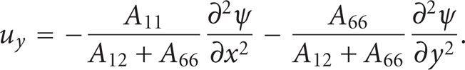
The above definition of ψ(x,y) satisfies the first equilibrium equation in (6) and (7) and the second equilibrium equation is reduced to

$\begin{array}{c}\frac{{\partial }^{\mathrm{4}}\psi }{\partial x^{\mathrm{4}}}+\left[\frac{A_{\mathrm{22}}}{A_{\mathrm{66}}}-\frac{A_{\mathrm{12}}^{\mathrm{2}}}{A_{\mathrm{11}}{A}_{\mathrm{66}}}-\frac{\mathrm{2}{A}_{\mathrm{12}}}{A_{\mathrm{11}}}\right]\frac{{\partial }^{\mathrm{4}}\psi }{\partial x^{\mathrm{2}}\partial y^{\mathrm{2}}}+\frac{A_{\mathrm{22}}}{A_{\mathrm{11}}}\frac{{\partial }^{\mathrm{4}}\psi }{\partial y^{\mathrm{4}}}=\mathrm{0}.\end{array}$

10

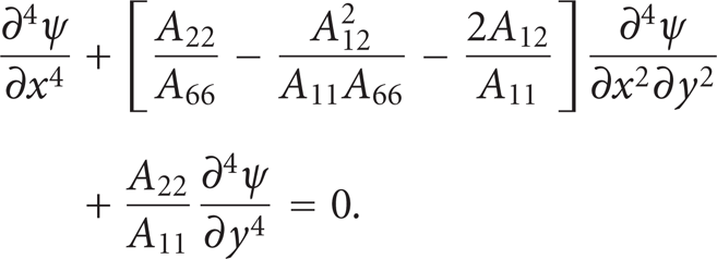
Now, one needs to satisfy only (10). By making use of (1), (8), (9), and strain-displacement relations, the components of stress can be expressed in terms of the same displacement potential function ψ(x,y) as

$\begin{array}{c}{\sigma }_x=\frac{A_{\mathrm{66}}}{h\left(A_{\mathrm{12}}+A_{\mathrm{66}}\right)}\left[A_{\mathrm{11}}\frac{{\partial }^{\mathrm{3}}\psi }{\partial x^{\mathrm{2}}\partial y}-A_{\mathrm{12}}\frac{{\partial }^{\mathrm{3}}\psi }{\partial y^{\mathrm{3}}}\right],\end{array}$

11

$\begin{array}{c}{\sigma }_y=\frac{\mathrm{1}}{h\left(A_{\mathrm{12}}+A_{\mathrm{66}}\right)}\times \left[\left(A_{\mathrm{12}}^{\mathrm{2}}+A_{\mathrm{12}}{A}_{\mathrm{66}}-A_{\mathrm{11}}{A}_{\mathrm{22}}\right)\frac{{\partial }^{\mathrm{3}}\psi }{\partial x^{\mathrm{2}}\partial y}-A_{\mathrm{22}}{A}_{\mathrm{66}}\frac{{\partial }^{\mathrm{3}}\psi }{\partial y^{\mathrm{3}}}\right],\end{array}$

12

$\begin{array}{c}{\sigma }_{xy}=\frac{A_{\mathrm{66}}}{h\left(A_{\mathrm{12}}+A_{\mathrm{66}}\right)}\left[A_{\mathrm{12}}\frac{{\partial }^{\mathrm{3}}\psi }{\partial x\partial y^{\mathrm{2}}}-A_{\mathrm{11}}\frac{{\partial }^{\mathrm{3}}\psi }{\partial x^{\mathrm{3}}}\right].\end{array}$

13

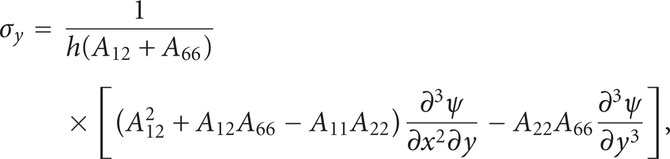
Equation (10) is a fourth-order partial differential equation for a single unknown function ψ(x,y). Once this equation is solved for ψ(x,y), the components of displacement and stress can readily be determined from (8), (9), (11), (12), and (13), respectively.

3. Cantilever Beam

3.1. Modelling of the Problem

The displacement potential formulations developed in the preceding sections are used to modelling a cantilever beam problem for the solution of elastic field due to a tip load. Figure 1 shows a thin deep cantilever beam of laminated composite with length b and height a. A Cartesian coordinate system x-y is considered with the origin located at the left lower corner of the beam and the x- and y-axes aligned with the longitudinal and lateral edges of the beam, respectively. The left lateral edge is rigidly fixed and the two longitudinal edges parallel to the x-axis are stiffened. As mentioned earlier, the application of stiffeners to structural elements is a common practice to improve the stiffness which, in turn, reduces the degree of deformation. The stiffeners are mathematically modelled by imposing zero deformation along their length [4–7]. The right lateral edge is subjected to a parabolic shear load ${\sigma }_{xy}^{\mathrm{0}}=\mathrm{4}P(y^{\mathrm{2}}-ay)/a^{\mathrm{2}}$ , where P is the maximum value of the stress at the center of the edge. It is noted that a load at the tip of a cantilever can be simulated as a parabolic shear load [1]. As the thickness of the cantilever is small in comparison with other dimensions, the analysis is carried out under plane stress condition. The relevant boundary conditions are

• $u_x(x,0)=u_x(x,a)=0;0\le x\le b$ (upper and lower stiffened edges),

• ${\sigma }_y(x,0)={\sigma }_y(x,a)=0;0\le x\le b$ (upper and lower stiffened edges),

• $u_x(0,y)=u_y(0,y)=0;0\le y\le a$ (left fixed edge),

• ${\sigma }_x(b,y)=0,{\sigma }_{xy}(b,y)={\sigma }_{xy}^0;0\le y\le a$ (right lateral edge).

Figure 1:

A cantilever beam of laminated composite under a parabolic shear load.

3.2. Solution of the Problem

To obtain the solution of the above cantilever beam problem, (10) should be solved for ψ(x,y) that must satisfy all the above boundary conditions. Here we assume the solution of (10) in the form of Fourier series as

$\begin{array}{c}\psi \left(x,y\right)={\sum }_{m=\mathrm{1}}^{\infty }{X}_m\left(x\right)\cos \alpha y+M{x}^{\mathrm{3}},\end{array}$

14

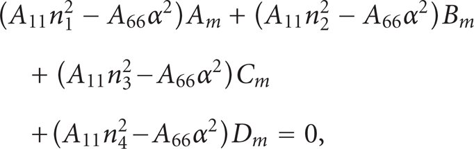
where X _m (x) is the function of x only, α = mπ/a, and M is an arbitrary constant. Note that any other expression for ψ(x,y) may also be assumed for the solution of (10). However, a simple expression with some additional benefits may be desirable. A close examination of (8), (12), and (14) shows that the boundary conditions (i) and (ii) on the stiffened edges are automatically satisfied by the expression of ψ(x,y) in (14), which are the additional benefits of our assumption. Now, the combination of (10) and (14) yields a fourth-order ordinary differential equation with constant coefficients as

$\begin{array}{c}{X}_m^{\mathrm{\prime \prime \prime \prime }}-{BX}_m^{\mathrm{\prime \prime }}{\alpha }^{\mathrm{2}}+CX{}_m{\alpha }_{}^{\mathrm{4}}=\mathrm{0},\end{array}$

(15)

where $B=(A_{\mathrm{22}}/A_{\mathrm{66}})-(A_{\mathrm{12}}^{\mathrm{2}}/A_{\mathrm{11}}{A}_{\mathrm{66}})-(\mathrm{2}{A}_{\mathrm{12}}/A_{\mathrm{11}})$ and $C=A_{\mathrm{22}}/A_{\mathrm{11}}$ . The general solution of (15) is

$\begin{array}{c}{X}_m=A_m{e}^{n_{\mathrm{1}}x}+B_m{e}^{n_{\mathrm{2}}x}+C_m{e}^{n_{\mathrm{3}}x}+D_m{e}^{n_{\mathrm{4}}x},\end{array}$

16

where

$\begin{array}{c}{n}_{\mathrm{1}},n_{\mathrm{2}}=\alpha \sqrt{\frac{(B\pm \sqrt{B^{\mathrm{2}}-\mathrm{4}C})}{\mathrm{2}}},\end{array}$

17

$\begin{array}{c}{n}_{\mathrm{3}},n_{\mathrm{4}}=-\alpha \sqrt{\frac{\left(B\pm \sqrt{B^{\mathrm{2}}-\mathrm{4}C}\right)}{\mathrm{2}}},\end{array}$

18

and A _m , B _m , C _m , and D _m are arbitrary constants. Now, by making use of (14) and (16) into (8), (9), (11), (12), and (13), the components of displacement and stress can be expressed as

$\begin{array}{c}{u}_x\left(x,y\right)={\sum }_{m=\mathrm{1}}^{\infty }[-(n_{\mathrm{1}}{A}_m{e}^{n_{\mathrm{1}}x}+n_{\mathrm{2}}{B}_m{e}^{n_{\mathrm{2}}x}\hspace{1em}\hspace{1em}\hspace{1em}\hspace{1em}\hspace{1em}+n_{\mathrm{3}}{C}_m{e}^{n_{\mathrm{3}}x}+n_{\mathrm{4}}{D}_m{e}^{n_{\mathrm{4}}x})\alpha \sin \alpha y],\end{array}$

19

$\begin{array}{cc}\text{(20)}& u_y\left(x,y\right)=\frac{\mathrm{1}}{A_{\mathrm{12}}+A_{\mathrm{66}}}\hspace{1em}\times {\sum }_{m=\mathrm{1}}^{\infty }[\{\phantom{+n_{\mathrm{3}}^{\mathrm{2}}{C}_m{e}^{n_{\mathrm{3}}x}+n_{\mathrm{4}}^{\mathrm{2}}{D}_m{e}^{n_{\mathrm{4}}x}}{A}_{\mathrm{66}}(A_m{e}^{n_{\mathrm{1}}x}+B_m{e}^{n_{\mathrm{2}}x}\hspace{1em}\hspace{1em}\hspace{1em}\hspace{1em}\hspace{1em}\hspace{1em}\hspace{1em}\hspace{1em}\hspace{1em}\hspace{1em}+C_m{e}^{n_{\mathrm{3}}x}+D_m{e}^{n_{\mathrm{4}}x}){\alpha }^{\mathrm{2}}\hspace{1em}\hspace{1em}\hspace{1em}\hspace{1em}\hspace{1em}-A_{\mathrm{11}}(n_{\mathrm{1}}^{\mathrm{2}}{A}_m{e}^{n_{\mathrm{1}}x}+n_{\mathrm{2}}^{\mathrm{2}}{B}_m{e}^{n_{\mathrm{2}}x}\hspace{1em}\hspace{1em}\hspace{1em}\hspace{1em}\hspace{1em}\hspace{1em}\hspace{1em}\hspace{1em}\hspace{1em}+n_{\mathrm{3}}^{\mathrm{2}}{C}_m{e}^{n_{\mathrm{3}}x}+n_{\mathrm{4}}^{\mathrm{2}}{D}_m{e}^{n_{\mathrm{4}}x})\}\hspace{1em}\hspace{1em}\hspace{1em}\hspace{1em}\hspace{1em}\times \cos \alpha y-\mathrm{6}Mx{A}_{\mathrm{11}}\phantom{A_m{e}^{n_{\mathrm{1}}x}+B_m{e}^{n_{\mathrm{2}}x}}],\end{array}$

20

$\begin{array}{c}{\sigma }_x\left(x,y\right)=-\frac{A_{\mathrm{66}}}{h\left(A_{\mathrm{12}}+A_{\mathrm{66}}\right)}\hspace{1em}\times {\sum }_{m=\mathrm{1}}^{\infty }[\phantom{n_{\mathrm{3}}^{\mathrm{2}}{C}_m{e}^{n_{\mathrm{3}}x}+n_{\mathrm{4}}^{\mathrm{2}}{D}_m{e}^{n_{\mathrm{4}}x}}{A}_{\mathrm{12}}(A_m{e}^{n_{\mathrm{1}}x}+B_m{e}^{n_{\mathrm{2}}x}\hspace{1em}+C_m{e}^{n_{\mathrm{3}}x}+D_m{e}^{n_{\mathrm{4}}x}){\alpha }^{\mathrm{3}}\hspace{1em}\hspace{1em}\hspace{1em}\hspace{1em}+A_{\mathrm{11}}(n_{\mathrm{1}}^{\mathrm{2}}{A}_m{e}^{n_{\mathrm{1}}x}+n_{\mathrm{2}}^{\mathrm{2}}{B}_m{e}^{n_{\mathrm{2}}x}+n_{\mathrm{3}}^{\mathrm{2}}{C}_m{e}^{n_{\mathrm{3}}x}+n_{\mathrm{4}}^{\mathrm{2}}{D}_m{e}^{n_{\mathrm{4}}x})\alpha ]\sin \alpha y,\end{array}$

21

$\begin{array}{c}{\sigma }_y\left(x,y\right)=-\frac{\mathrm{1}}{h\left(A_{\mathrm{12}}+A_{\mathrm{66}}\right)}\hspace{1em}\times {\sum }_{m=\mathrm{1}}^{\infty }[\phantom{+n_{\mathrm{4}}^{\mathrm{2}}{D}_m{e}^{n_{\mathrm{4}}x}}{A}_{\mathrm{22}}{A}_{\mathrm{66}}(A_m{e}^{n_{\mathrm{1}}x}+B_m{e}^{n_{\mathrm{2}}x}\hspace{1em}\hspace{1em}\hspace{1em}\hspace{1em}\hspace{1em}\hspace{1em}\hspace{1em}\hspace{1em}\hspace{1em}+C_m{e}^{n_{\mathrm{3}}x}+D_m{e}^{n_{\mathrm{4}}x}){\alpha }^{\mathrm{3}}\hspace{1em}\hspace{1em}\hspace{1em}\hspace{1em}+\left(A_{\mathrm{12}}^{\mathrm{2}}+A_{\mathrm{12}}{A}_{\mathrm{66}}-A_{\mathrm{11}}{A}_{\mathrm{22}}\right)\hspace{1em}\hspace{1em}\hspace{1em}\hspace{1em}\times (n_{\mathrm{1}}^{\mathrm{2}}{A}_m{e}^{n_{\mathrm{1}}x}+n_{\mathrm{2}}^{\mathrm{2}}{B}_m{e}^{n_{\mathrm{2}}x}+n_{\mathrm{3}}^{\mathrm{2}}{C}_m{e}^{n_{\mathrm{3}}x}\hspace{1em}\hspace{1em}\hspace{1em}\hspace{1em}\hspace{1em}\hspace{1em}+n_{\mathrm{4}}^{\mathrm{2}}{D}_m{e}^{n_{\mathrm{4}}x})\alpha ]\sin \alpha y,\end{array}$

22

$\begin{array}{c}{\sigma }_{xy}\left(x,y\right)=-\frac{A_{\mathrm{66}}}{h\left(A_{\mathrm{12}}+A_{\mathrm{66}}\right)}\hspace{1em}\times {\sum }_{m=\mathrm{1}}^{\infty }[\phantom{+n_{\mathrm{3}}^{\mathrm{3}}{C}_m{e}^{n_{\mathrm{3}}x}+n_{\mathrm{4}}^{\mathrm{3}}{D}_m{e}^{n_{\mathrm{4}}x}}{A}_{\mathrm{12}}(n_{\mathrm{1}}{A}_m{e}^{n_{\mathrm{1}}x}+n_{\mathrm{2}}{B}_m{e}^{n_{\mathrm{2}}x}\hspace{1em}\hspace{1em}\hspace{1em}\hspace{1em}\hspace{1em}\hspace{1em}\hspace{1em}\hspace{1em}+n_{\mathrm{3}}{C}_m{e}^{n_{\mathrm{3}}x}+n_{\mathrm{4}}{D}_m{e}^{n_{\mathrm{4}}x}){\alpha }^{\mathrm{2}}\hspace{1em}\hspace{1em}\hspace{1em}\hspace{1em}\hspace{1em}+A_{\mathrm{11}}(n_{\mathrm{1}}^{\mathrm{3}}{A}_m{e}^{n_{\mathrm{1}}x}+n_{\mathrm{2}}^{\mathrm{3}}{B}_m{e}^{n_{\mathrm{2}}x}\hspace{1em}\hspace{1em}\hspace{1em}\hspace{1em}\hspace{1em}\hspace{1em}\hspace{1em}\hspace{1em}\hspace{1em}+n_{\mathrm{3}}^{\mathrm{3}}{C}_m{e}^{n_{\mathrm{3}}x}+n_{\mathrm{4}}^{\mathrm{3}}{D}_m{e}^{n_{\mathrm{4}}x})]\cos \alpha y\hspace{1em}-\frac{\mathrm{6}M{A}_{\mathrm{11}}{A}_{\mathrm{66}}}{h\left(A_{\mathrm{12}}+A_{\mathrm{66}}\right)}.\end{array}$

23

As mentioned earlier, the boundary conditions (i) and (ii) are satisfied automatically. Thus, the boundary conditions (iii) and (iv) are remaining to be satisfied. Before application of the boundary conditions (iii) and (iv), the parabolic shear load applied to the edge x = b is expressed in terms of Fourier series as

$\begin{array}{c}{\sigma }_{xy}^{\mathrm{0}}\left(b,y\right)=E_{\mathrm{0}}+{\sum }_{m=\mathrm{1}}^{\infty }{E}_m\cos \alpha y,\end{array}$

24

where E₀ = −2P/3 and $E_m=\mathrm{8}P[\mathrm{1}+\cos (m\pi )]/m^{\mathrm{2}}{\pi }^{\mathrm{2}}$ . Now, applying the boundary conditions (iii) and (iv) into (19), (20), (21), and (23), one obtains the constant M as

$\begin{array}{c}M=\frac{hP\left(A_{\mathrm{12}}+A_{\mathrm{66}}\right)}{\mathrm{9}{A}_{\mathrm{11}}{A}_{\mathrm{66}}},\end{array}$

25

and the following four simultaneous equations for the determination of the constants A _m , B _m , C _m , and D _m :

$\begin{array}{c}{n}_{\mathrm{1}}{A}_m+n_{\mathrm{2}}{B}_m+n_{\mathrm{3}}{C}_m+n_{\mathrm{4}}{D}_m=\mathrm{0},\hspace{1em}\mathrm{0}<y<a,\end{array}$

26

$\left(A_{\mathrm{11}}{n}_{\mathrm{1}}^{\mathrm{2}}-A_{\mathrm{66}}{\alpha }^{\mathrm{2}}\right)A_m+\left(A_{\mathrm{11}}{n}_{\mathrm{2}}^{\mathrm{2}}-A_{\mathrm{66}}{\alpha }^{\mathrm{2}}\right)B_m\hspace{1em}+\left(A_{\mathrm{11}}{n}_{\mathrm{3}}^{\mathrm{2}}-A_{\mathrm{66}}{\alpha }^{\mathrm{2}}\right)C_m\hspace{1em}+\left(A_{\mathrm{11}}{n}_{\mathrm{4}}^{\mathrm{2}}-A_{\mathrm{66}}{\alpha }^{\mathrm{2}}\right)D_m=\mathrm{0},$

27

$\begin{array}{c}\left(A_{\mathrm{11}}{n}_{\mathrm{1}}^{\mathrm{2}}\alpha +A_{\mathrm{12}}{\alpha }^{\mathrm{3}}\right)A_m{e}^{n_{\mathrm{1}}b}+\left(A_{\mathrm{11}}{n}_{\mathrm{2}}^{\mathrm{2}}\alpha +A_{\mathrm{12}}{\alpha }^{\mathrm{3}}\right)B_m{e}^{n_{\mathrm{2}}b}\hspace{1em}+\left(A_{\mathrm{11}}{n}_{\mathrm{3}}^{\mathrm{2}}\alpha +A_{\mathrm{12}}{\alpha }^{\mathrm{3}}\right)C_m{e}^{n_{\mathrm{3}}b}\hspace{1em}+\left(A_{\mathrm{11}}{n}_{\mathrm{4}}^{\mathrm{2}}\alpha +A_{\mathrm{12}}{\alpha }^{\mathrm{3}}\right)D_m{e}^{n_{\mathrm{4}}b}=\mathrm{0},\end{array}$

28

$\begin{array}{c}\left(A_{\mathrm{11}}{n}_{\mathrm{1}}^{\mathrm{3}}+A_{\mathrm{12}}{n}_{\mathrm{1}}{\alpha }^{\mathrm{2}}\right)A_m{e}^{n_{\mathrm{1}}b}+\left(A_{\mathrm{11}}{n}_{\mathrm{2}}^{\mathrm{3}}+A_{\mathrm{12}}{n}_{\mathrm{2}}{\alpha }^{\mathrm{2}}\right)B_m{e}^{n_{\mathrm{2}}b}\hspace{1em}+\left(A_{\mathrm{11}}{n}_{\mathrm{3}}^{\mathrm{3}}+A_{\mathrm{12}}{n}_{\mathrm{3}}{\alpha }^{\mathrm{2}}\right)C_m{e}^{n_{\mathrm{3}}b}+\left(A_{\mathrm{11}}{n}_{\mathrm{4}}^{\mathrm{3}}+A_{\mathrm{12}}{n}_{\mathrm{4}}{\alpha }^{\mathrm{2}}\right)D_m{e}^{n_{\mathrm{4}}b}\hspace{1em}=\frac{-E_{m}h\left(A_{\mathrm{12}}+A_{\mathrm{66}}\right)}{A_{\mathrm{66}}}.\end{array}$

29

The constants A _m , B _m , C _m , and D _m obtained from the above equations are substituted into (19), (20), (21), (22), and (23) to obtain the explicit expressions of displacement and stress which are valid to the entire region of the cantilever beam.

4. Results and Discussion

The modelling of the present cantilever beam problem is demonstrated for glass/epoxy laminated composites. The properties of an orthotropic unidirectional glass/epoxy composite lamina are shown in Table 1. These properties are used in calculating the laminate properties of interest. All the results presented in this section correspond to the aspect ratio of the beam b/a = 3.0. The maximum value of the applied load P is taken as 1000 MPa and the thickness of each ply is considered to be 1.0 mm. The convergence of the series solution is ensured by comparing the results for different values of the number of terms m in the series. It is found that the results converge very well for m = 5 only. However, for further accuracy, 10 terms in the series have been used to generate all the results presented hereafter.

Table 1:

Mechanical properties of a glass/epoxy unidirectional lamina.

E1 (MPa)	E2 (MPa)	G12 (MPa)	ν 12	ν 21
38.60 × 103	8.27 × 103	4.14 × 103	0.26	0.06

Figure 2 shows the normalized longitudinal displacement u _x /b at different sections of the cantilever beam as a function of normalised position y/a. The beam consists of a cross-ply laminate with laminate stacking sequence [0/90/0]. Unless otherwise stated, all the results from this point forward correspond to the beam of cross-ply laminate [0/90/0]. As seen, the displacement is zero at the section x/b = 0 and at the top (y/a = 1.0) and bottom (y/a = 0) edges of the cantilever. This satisfies the physical boundary conditions of the problem. The maximum displacement occurs at the right lateral edge (x/b = 1.0) and it gradually decreases towards the fixed support (x/b = 0). Shown in Figure 3 is the normalized lateral displacement (u _y /a) at different sections of the beam. The lateral displacement is also exactly zero at the fixed support (x/b = 0) which satisfies the boundary conditions of the problem. The magnitude of this displacement is also the maximum at the right lateral edge and gradually diminishes towards the fixed support. Further, the variation of the displacement with y/a is almost zero at all the sections except the right lateral edge x/b = 1.0. However, the magnitude of the displacement varies significantly from one section to another section, that is, with the variation of x/b.

Figure 2:

Longitudinal displacement at different sections of the cross-ply composite beam.

Figure 3:

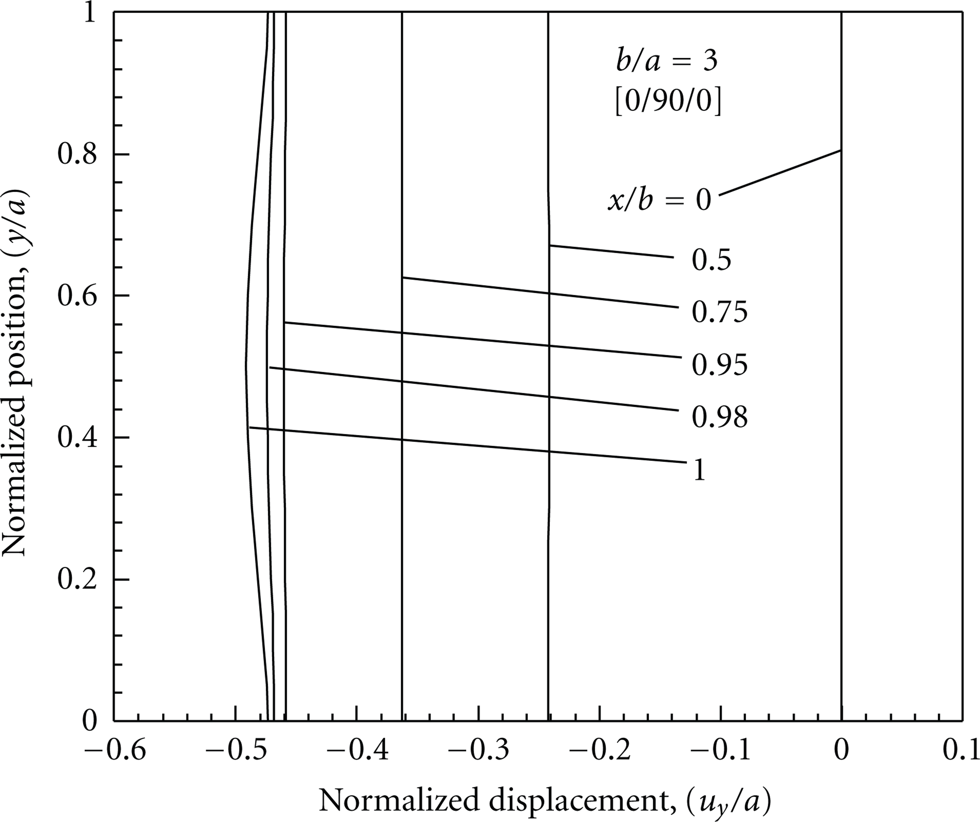
Lateral displacement at different sections of the cross-ply composite beam.

The distribution of normalized longitudinal stress component (σ _x /P) as a function of normalized position (y/a) is illustrated in Figure 4. At the right lateral edge (x/b = 1.0), the stress is zero that satisfies the boundary condition of the problem. Further, the longitudinal stress is zero at the fixed support and at the top and bottom stiffened edges of the cantilever. The magnitude of the stress is maximum near the right lateral edge (x/b = 0.95) of the cantilever and it gradually decreases towards the fixed support. The distribution of this stress component shows that the neutral axis coincides with the geometric mid-plane y/a = 0.5, where stress is zero for any section (any value of x/b). The normalized lateral stress component ((σ _y /P)) is displayed in Figure 5. The distribution of this stress component is similar to that of the longitudinal stress component except that this stress is the maximum at the right lateral edge. Figure 6 depicts the distribution of normalized shear stress component (σxy/ _P ). At the right lateral edge (x/b = 1.0), the distribution of the shear stress exactly matches with the applied load. For the sections near the right lateral edge (e.g., x/b = 0.98), the magnitude of the shear stress is the maximum at the mid-plane (y/a = 0.5) which decreases towards the top and bottom edges of the beam. This scenario changes for the sections away from the right lateral edge of the beam. More specifically, the magnitude of this stress component is the minimum at the mid-plane (y/a = 0.5) which increases towards the top and bottom edges of the beam as seen for the sections x/b = 0.9 and 0.75.

Figure 4:

Longitudinal stress at different sections of the cross-ply composite beam.

Figure 5:

Lateral stress at different sections of the cross-ply composite beam.

Figure 6:

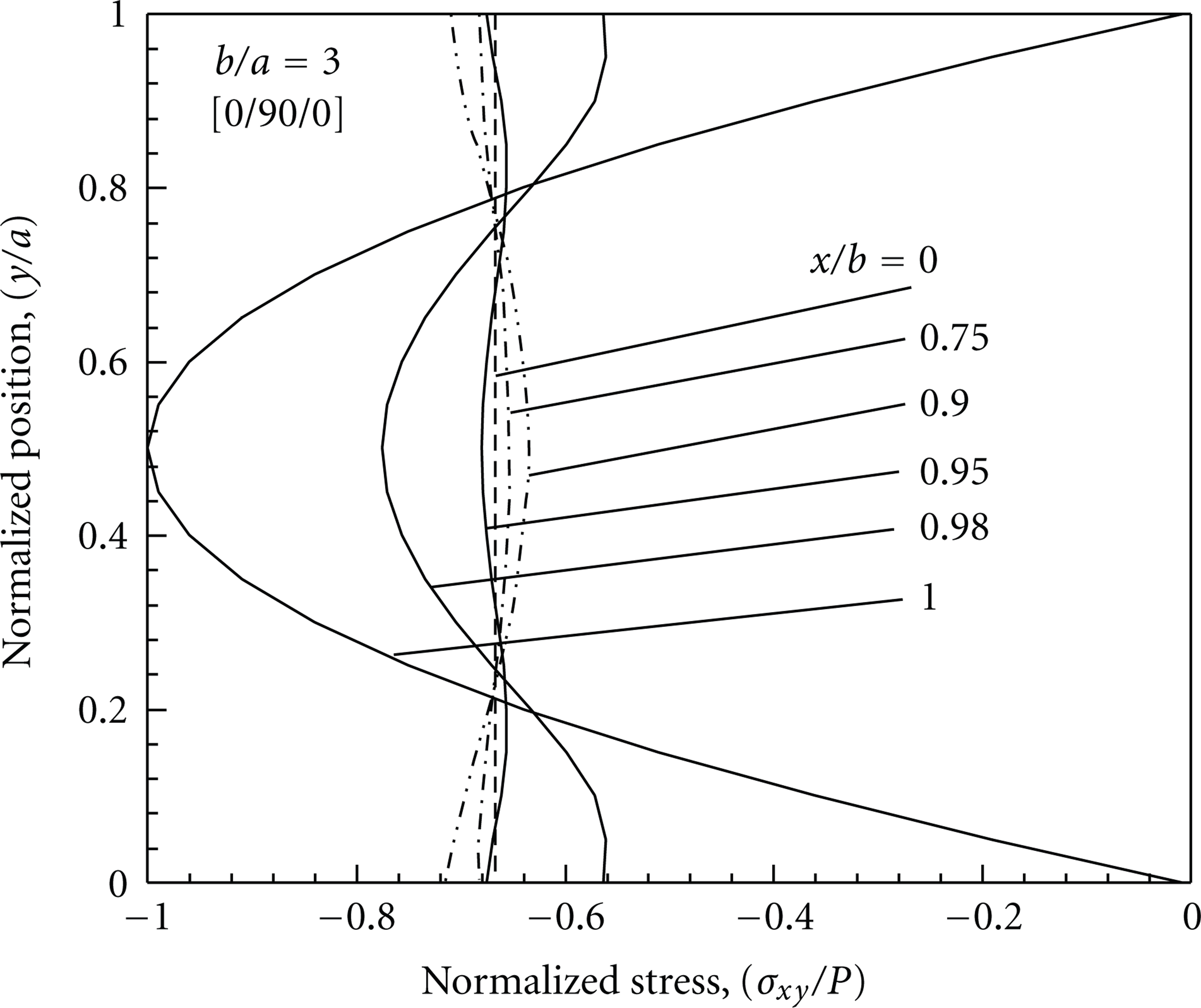
Shear stress at different sections of the cross-ply composite beam.

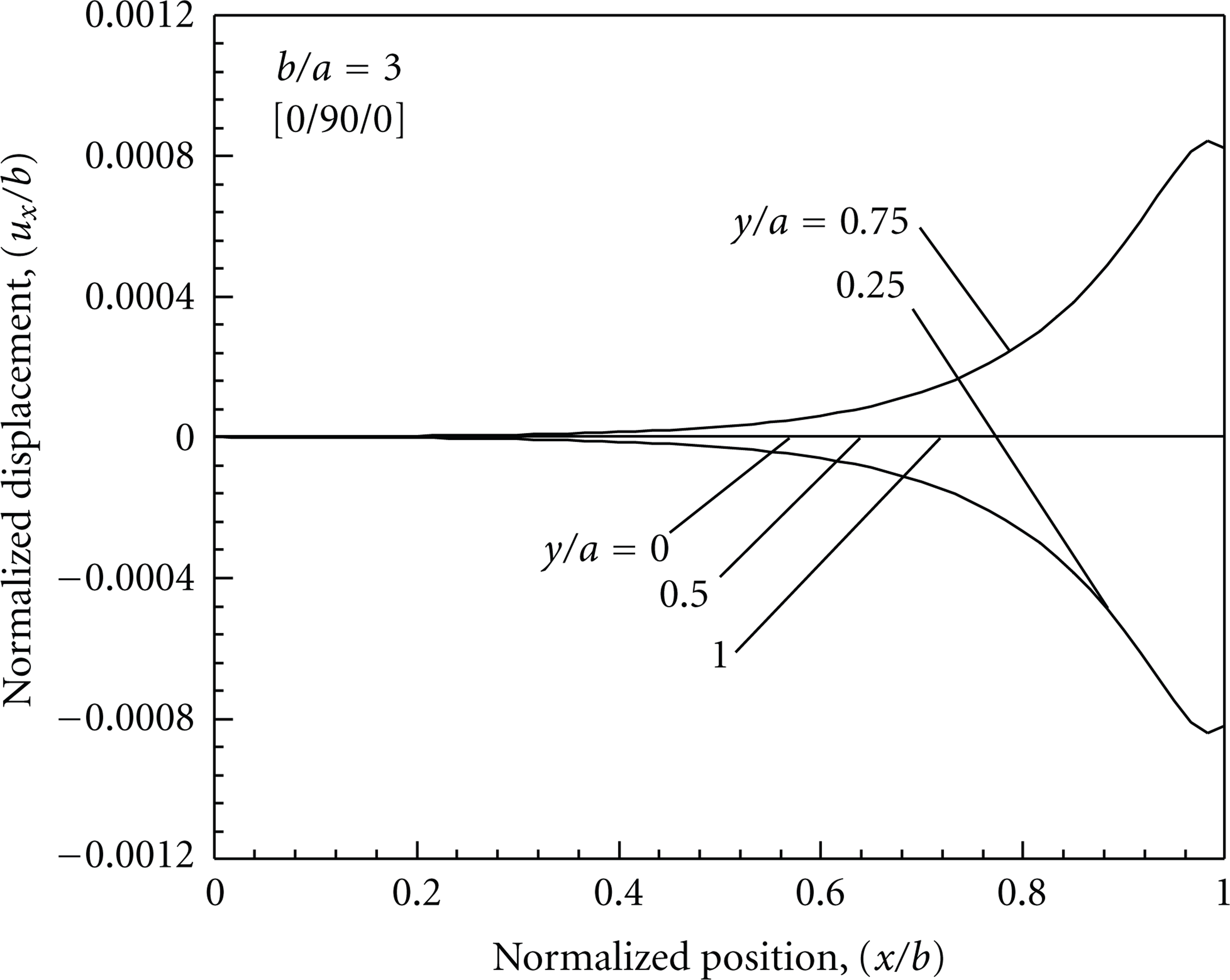
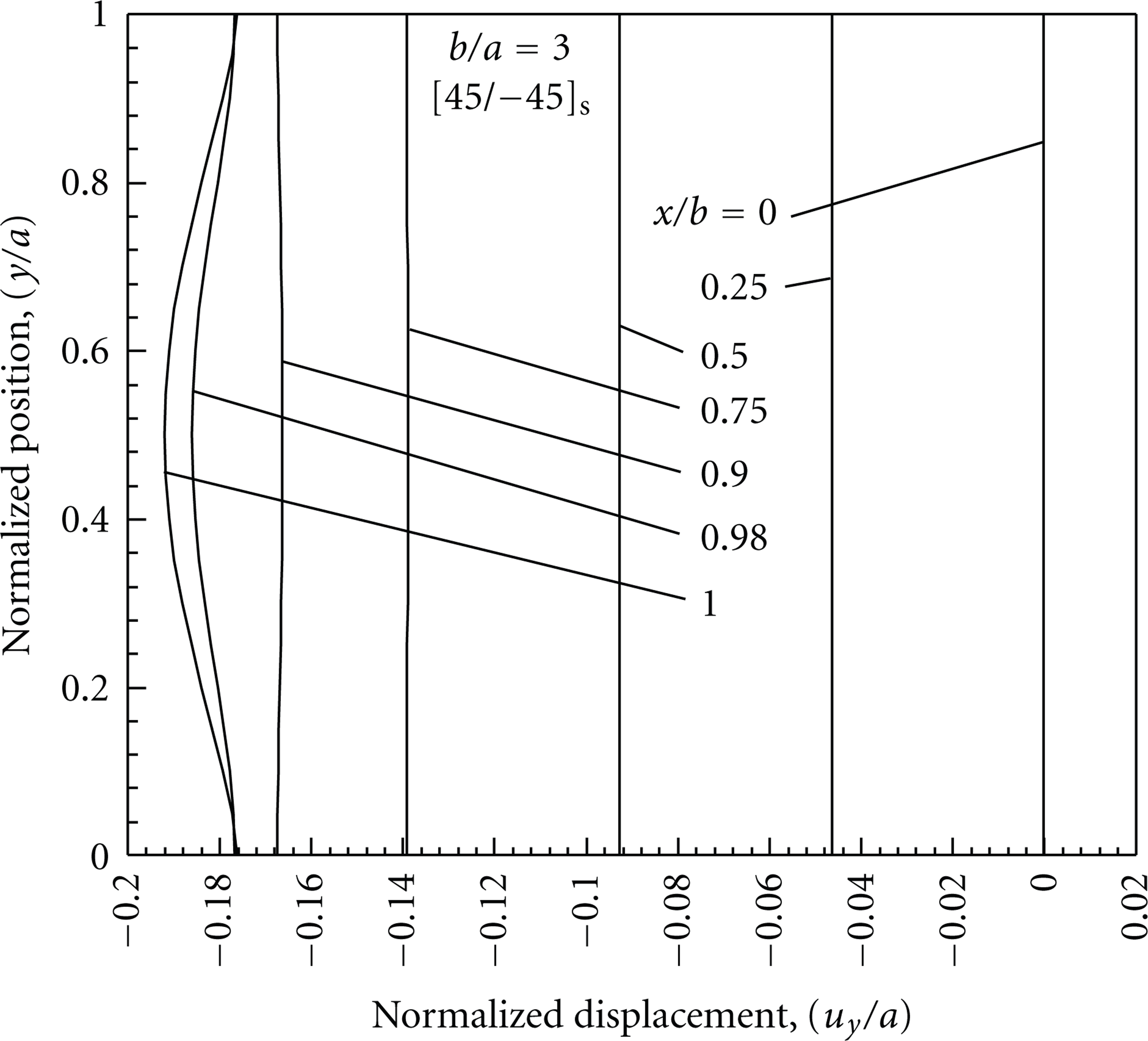
The distribution of displacement and stress along the longitudinal direction of the beam is illustrated in Figures 7 to 11. The longitudinal displacement u _x /b is zero along the entire mid-plane (y/a = 0.5), which is the neutral axis of the beam. Further, the displacement is zero along the top (y/a = 1.0) and bottom (y/a = 0) edges of the beam, which conforms to the boundary condition of the present stiffened beam problem. However, at other longitudinal sections between the neutral plane and top or bottom edge of the beam, this displacement component varies with x/b as shown by the curves corresponding to y/a = 0.25 and 0.75. The variation is substantial at the right half of the beam, particularly at and near the right edge of the beam. Further, the distribution of the displacement is symmetric with respect to the neutral axis of the beam. The lateral displacement component u _y /b as a function of x/b at different longitudinal sections is illustrated in Figure 8. The distribution of this displacement component is the same for any section except the small region of x/b > 0.96 where a small variation of the displacement from one longitudinal section to another can be observed.

Figure 7:

Longitudinal displacement at different sections of the cross-ply composite beam.

Figure 8:

Lateral displacement at different sections of the cross-ply composite beam.

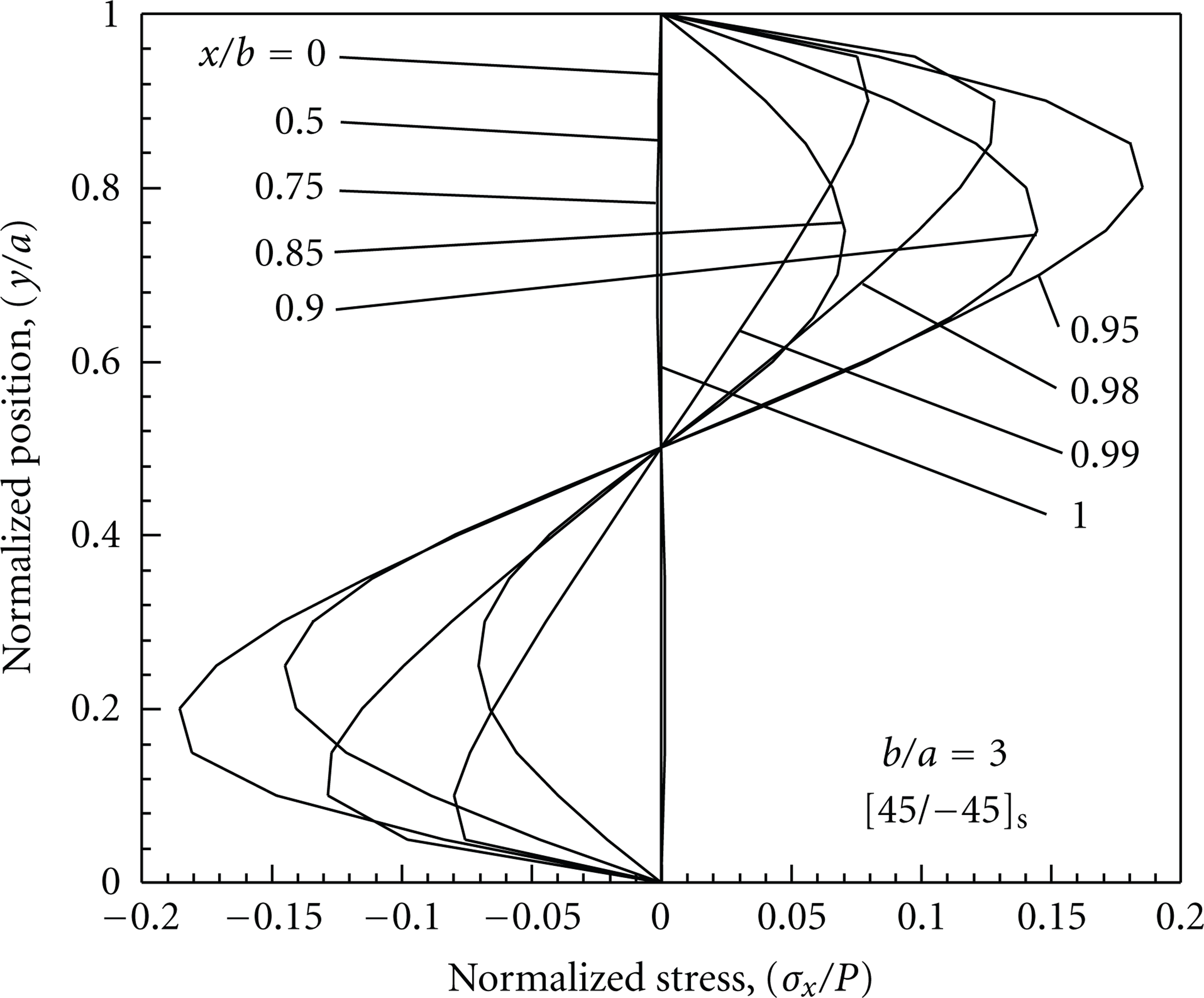
The longitudinal stress distribution along the longitudinal direction of the beam as shown in Figure 9 is similar to that of the longitudinal displacement except that the stress is zero for any value ofy/aat the right lateral edge x/b = 1.0. The lateral stress (σ _y /P) varies from one section to another section (except the sections (y/a = 0), 0.5, and 1.0) only for x/b > 0.92 as can be seen from Figure 10. The distribution of the shear stress component along the longitudinal direction is shown in Figure 11. Unlike longitudinal and lateral stress components, the shear stress is nonzero at any section of the beam. From the fixed end to x/b = 0.6, the stress does not vary with x/b. A close observation shows that the stress distribution at the right lateral edge (x/b = 1.0) conforms to the parabolic applied load at that edge. At (y/a = 0) and 1.0, the stress is zero and its value is maximum and equal to the applied load P at y/a = 0.5.

Figure 9:

Longitudinal stress at different sections of the cross-ply composite beam.

Figure 10:

Lateral stress at different sections of the cross-ply composite beam.

Figure 11:

Shear stress at different sections of the cross-ply composite beam.

To investigate the effect of laminate stacking sequence of a cross-ply laminate consisting of three plies on the elastic field, four different stacking sequences, $[0/0/0]$ , $[0/90/0]$ , $[90/0/90]$ , and $[90/90/90]$ , are considered. Only the results of the vertical section x/b = 0.75 are shown in Figures 12 to 16. Figure 12 shows that the peak values of longitudinal displacement occur at y/a = 0.25 and 0.75 for any stacking sequence. These peak values are found to decrease as the number of 90 degree plies increases. The value of lateral displacement is maximum at the bottom ((y/a = 0)) and top ((y/a = 0)) surfaces of the beam when all the plies have 0 degree orientation as can be seen from Figure 13. The maximum value decreases as the number of90 degree plies increases. Further, the minimum value of lateral displacement is obtained at y/a = 0.5 when all the plies have 0 degree orientation. As the number of 90 degree plies increases, the value of lateral displacement increases aty/a = 0.5. The longitudinal stress shown in Figure 14 exhibits the similar characteristics as the longitudinal displacement displayed in Figure 12. Shown in Figure 15 is the lateral stress as a function of laminate stacking sequence. This stress component has similar characteristics as the longitudinal stress of Figure 14 except that the positive and negative stresses interchange their position between y/a = 0.25 and 0.75. The effect of laminate stacking sequence on the shear stress component is illustrated in Figure 16. The characteristics of these stresses are similar to those of lateral displacement shown in Figure 13.

Figure 12:

Effect of laminate stacking sequence on longitudinal displacement.

Figure 13:

Effect of laminate stacking sequence on lateral displacement.

Figure 14:

Effect of laminate stacking sequence on longitudinal stress.

Figure 15:

Effect of laminate stacking sequence on lateral stress.

Figure 16:

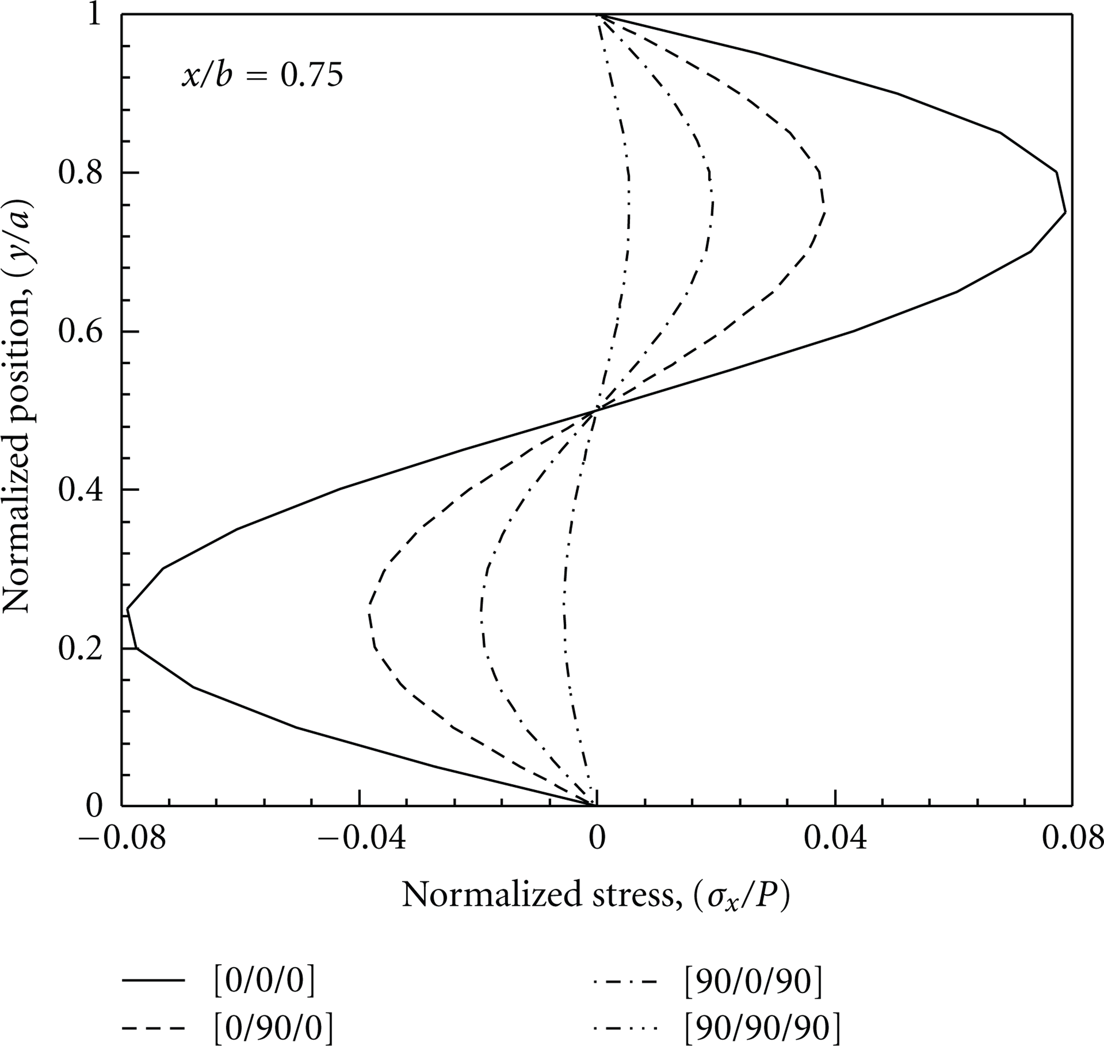
Effect of laminate stacking sequence on shear stress.

In the preceding paragraphs, the results presented correspond to the cantilever beam of cross-ply laminate. Now some results will be presented and discussed for the beam of [45/ – 45] _s angle-ply laminate.

Figure 17 displays the distribution of normalized longitudinal displacement component u _x /b as a function of y/a at different lateral sections of the beam. It shows a bit different characteristics than the case of the cross-ply laminated beam at and near the right lateral edge. For the angle-ply laminated beam, the longitudinal displacement is not maximum at the right lateral edge x/b = 1.0. Rather, the maximum value of the displacement occurs at a section (e.g., x/b = 0.95) near the right lateral edge x/b = 1.0. For the sections in the region x/b < 0.95, the characteristics of the displacement are similar to the case of the cross-ply beam, that is, the value of the displacement decreases towards the fixed edge. The normalized lateral displacement shown in Figure 18 exhibits exactly similar characteristics to that of the cross-ply cantilever beam.

Figure 17:

Longitudinal displacement at different sections of the angle-ply composite beam.

Figure 18:

Lateral displacement at different sections of the angle-ply composite beam.

The normalized longitudinal stress (σ _x /P) as a function of y/a is exhibited in Figure 19. At the right lateral edge x/b = 1.0, the stress is zero that increases towards the fixed support until the value of x/b = 0.95. After this, the magnitude of this stress decreases as a section further moves towards the fixed support (x/b = 0). The distribution of the normalized lateral stress (σ _y /P) as a function of y/a at different sections of the beam as shown in Figure 20 is similar to that of the cross-ply cantilever beam, that is, the magnitude of the stress is the maximum at the right lateral edge x/b = 1.0, which gradually decreases to zero as the fixed support is approached. Shown in Figure 21 is the distribution of normalized shear stress σxy/P that shows the characteristics similar to that of the cross-ply cantilever beam. Note that, like longitudinal and lateral stress components, the shear stress is not zero at the fixed support (x/b = 0) for both the cases of cross-ply and angle-ply beams.

Figure 19:

Longitudinal stress at different sections of the angle-ply composite beam.

Figure 20:

Lateral stress at different sections of the angle-ply composite beam.

Figure 21:

Shear stress at different sections of the angle-ply composite beam.

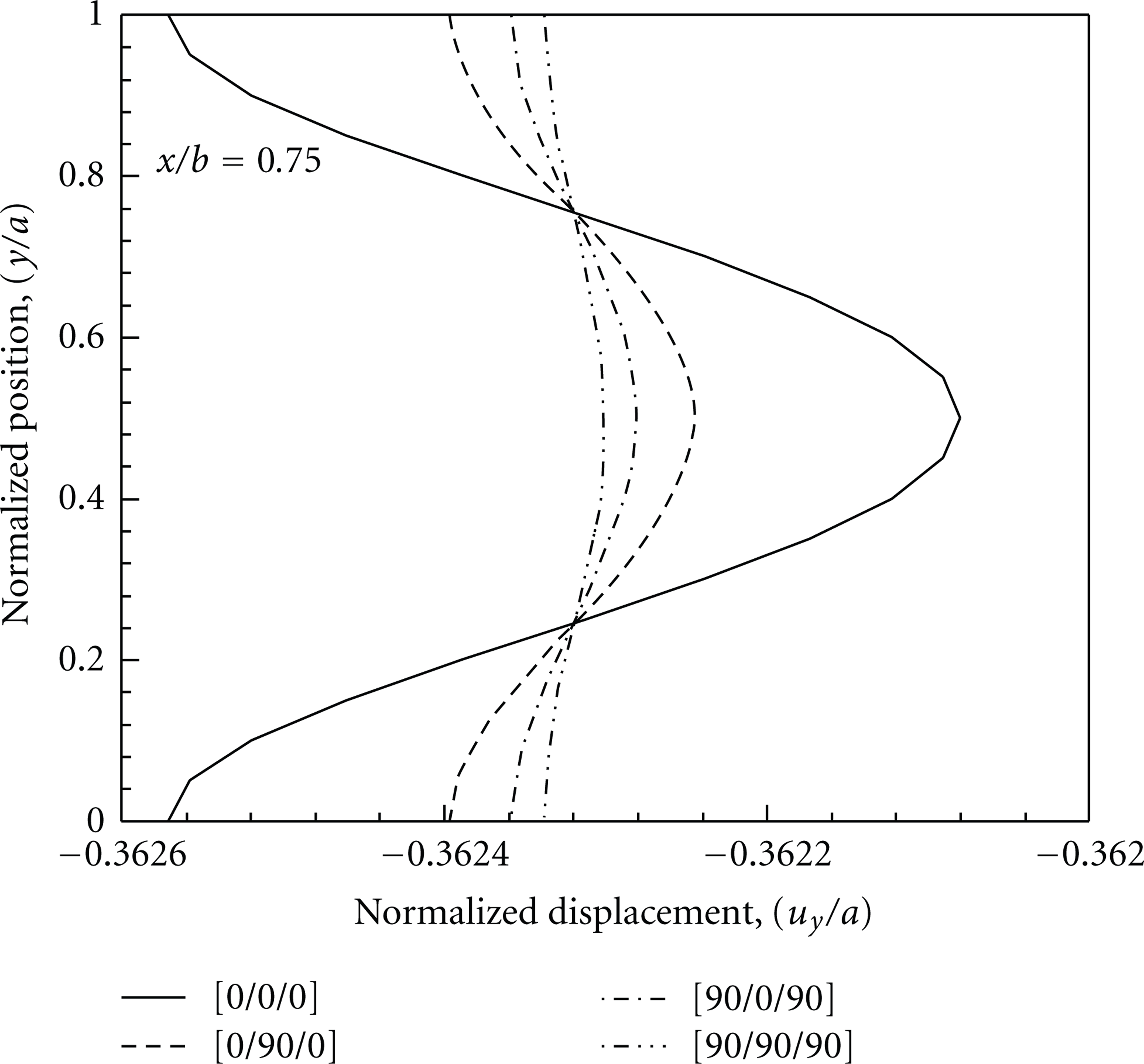
To investigate the effect of ply-angle on the elastic field in the case of the angle-ply cantilever beam, three different pointsy/a = 0.25, 0.50, and 0.75 on the lateral section x/b = 0.75 are considered for which results are computed as a function of ply-angle θ varying from 0 to 90 degrees. Figure 22 illustrates the variation of normalized longitudinal displacement with the variation of ply-angle θ which shows that the displacement at the mid-longitudinal plane, y/a = 0.5, is zero and remains uninfluenced by the ply-angle θ. However, near the top (y/a = 0.75) and bottom (y/a = 0.25) surfaces of the beam, the longitudinal displacement varies significantly as the ply-angle varies from 0 to about 40 degrees. With further increase of the ply-angle, the variation of the displacement is insignificant. Also, the displacement at any point along the lateral section x/b = 0.75 is zero for the ply-angle 40 and 60 degrees. Further, it is noted that the value of the displacement is the maximum for y/a = 0.25 and 0.75 when the ply-angle is zero, which implies the unidirectional composite. This conforms to the results corresponding to the [0/0/0] curve as shown in Figure 12. Thus, zero degree is the critical ply-angle in terms of longitudinal displacement. The normalized lateral displacement is shown in Figure 23 that gives the information that the magnitude and variation of this displacement component with the variation of ply-angle is the same at any point along a lateral section (e.g., x/b = 0.75). The magnitude of the lateral displacement is the minimum at θ = 45 degrees and its value increases as the ply-angle deviates in either direction from 45 degrees.

Figure 22:

Effect of ply-angle on longitudinal displacement.

Figure 23:

Effect of ply-angle on lateral displacement.

The normalized longitudinal stress component as shown in Figure 24 has the similar characteristics to that of the longitudinal displacement component shown in Figure 22. However, the lateral stress component as shown in Figure 25 has a completely different characteristic than lateral displacement. The lateral stress at the mid-point (y/a = 0.5) of the lateral section x/b = 0.75 is uninfluenced by the ply-angle which always remains zero. However, near the top and bottom surfaces of the beam, the magnitude of the stress increases as the ply-angle varies from 0 to about 35 degrees. Then it falls as the ply-angle further increases. In terms of the lateral stress, θ = 37 degree is the critical ply-angle for which the value of the lateral stress near the top (y/a = 0.75) and bottom (y/a = 0.25) surfaces is the maximum.

Figure 24:

Effect of ply-angle on longitudinal stress.

Figure 25:

Effect of ply-angle on lateral stress.

Shown in Figure 26 is the effect of ply-angle on the shear stress component. The shear stress exhibits the reverse trend to that of the longitudinal and lateral stress components. In this case, the stress at the mid-point (y/a = 0.5) of the vertical section x/b = 0.75 has a significant variation with the variation of the ply-angle. On the contrary, the stress near the top and bottom surfaces of the beam has a little variation with the ply-angle. In addition, the shear stress at the points of equal distance from the mid-point of the vertical section is exactly the same. Note that, in terms of shear stress, θ = 34 degree is the critical value of the ply-angle for which the stress is the maximum.

Figure 26:

Effect of ply-angle on shear stress.

5. Conclusion

A stiffened cantilever beam of symmetric laminated composite is mathematically modelled in terms of a single displacement potential function for analytical solution to elastic field in the beam under mixed boundary conditions. The model is suitable for any boundary conditions prescribed in terms of either stress or constraints or any combination of them. The numerical results obtained for a glass/epoxy laminated composite beam show that all the boundary conditions are satisfied exactly. This justifies that the present model is reliable as well as simple in obtaining analytical solution to elastic field even in the critical regions of supports and loadings of structural elements of laminated composites under mixed boundary conditions. From the numerical results of the stiffened cantilever beam, the following major conclusions can be made.

1. The analysis of the cross-ply cantilever beam shows that the beam with all the 90-degree plies is much better than that with all the zero-degree plies in terms of all the components of stress and displacement.

2. For the cantilever made of angle-ply laminated composite, ply-angle is an important parameter that has a significant effect on the elastic field. The same value of the ply-angle does not correspond to the critical value for all the components of stress and displacement. Therefore, to design with a cantilever beam of angle-ply laminate, it is necessary to find out an optimum value of the ply-angle for which all the components of stress and displacement can be minimized to a desired level.