The Role of Nodes Distribution in Extending the Lifetime of Wireless Sensor Networks

Abstract

One of the most important issues in sensor networks is prolonging the network lifetime. In this paper, we demonstrate that given a constant number of nodes, how distribution of nodes affects the lifetime. For this purpose, we first show that in a network with cluster-based routing protocol, nodes do not have equal importance, and their importance depends on their location, and we determine the most critical regions. We prove that the uniform distribution of nodes is not a good distribution. Finally, we propose a solution for the best distribution that concentrates the population of nodes on critical areas. Simulation results of our proposed distribution show a remarkable increase in network lifetime.

1. Introduction

A sensor network consists of a large number of sensor nodes deployed over an area. Nodes are low cost and are usually equipped with a power supply, a microprocessor, microsensors, and radio component that provides for wireless communication between nodes. This set of nodes is used for a variety of applications. The most common use is to monitor changes in a special parameter in a region. For instance, in [1], the temperature and humidity of different elevations of a tree are measured over a period of time, or, in [2], the environment of a coalmine is monitored by a wireless sensor network.

The most distinctive characteristic of a sensor network is the limited energy supply available for each node (a typical battery) due to their small size. Moreover, because of their size and low cost it would not be beneficial to recharge or replace the depleted battery of the nodes. In other words, every node is deemed useless after its battery discharges; therefore, finding energy-efficient routing protocols has become a significant issue. Flooding and gossiping [3], SPIN [4], LEACH [5], and HEED [6] are some examples of routing protocols proposed in the literature.

One of the most well-known techniques is clustering in which nodes are divided into groups called clusters with a node assigned as the cluster head. This technique prevents long-distance communication from distant nodes to the base station, thus, manages to save considerable amounts of energy. Instead, nodes included in a cluster communicate directly with their cluster head, and cluster heads forward the information to the base station within one-hop or multihop routes [7–10]. Clustering algorithms vary mainly based on their number of cluster heads, methods to form a cluster, cluster head election techniques, intercluster communications, and so forth.

One of the primary goals of all mentioned methods is to extend the time that the network is functioning as expected for its specific application. The effective lifetime has been defined in different ways. In [11], life time is defined as the time period for the first node to run out of its energy reserve. Authors of [12] define lifetime as the time until the first failure of the packet delivery due to battery outage. Definition of lifetime in [13] is the time for which 100% or 90% of the network coverage is preserved.

In a given routing algorithm, several parameters directly affect the performance of the network, such as number of the nodes, the area that needs to be observed, the mobility of nodes, and so forth. One of the most effective factors is the distribution of the nodes. The position of the nodes relative to each other and the base station can greatly influence the effective lifetime of the network.

In this paper, we are going to study the relation between the distribution of nodes over the monitored area and network's lifetime. Here, we consider lifetime to be the period that the network's coverage remains at more than 90% of its initial value. Then, we will try to extract the optimum solution for distributing the nodes.

2. Related Works

Several researches have been done addressing the issue of distribution in WSNs. Authors of [14] show how to improve the total data capacity of WSNs by using nonuniform sensor deployment strategy. In [14], SSEP model (Single Static Sink Edge Placement) is discussed in which nodes are placed uniformly in a rectangular area, and base station is located on one of the edges of this rectangle. The performance of such model is measured against the SSEP-NU (SSEP with nonuniform distribution) model for the network. Finally, it is shown that using the SSEP-NU model along with a mobile sink and a suitable routing protocol can improve the total data capacity by one order of magnitude compared to the original SSEP model. The authors extend their models in [15], where they introduce SSEP-NS (SSEP with nonuniform sensor distribution) model. In [16], another nonuniform distribution is suggested in order to avoid unbalanced energy depletion in the network. In this work, it is assumed that all the nodes are deployed in a circular area with a radius of R, and the base station is located in the center. The area around the base station is divided into R adjacent coronas with the same width of 1 unit. In the proposed nonuniform node distribution strategy, number of nodes increases with geometric proportion from the outer parts to the inner ones. The ratio between the node densities of the adjacent ${(i+1)}_{\text{th}}$ corona and the $i_{\text{th}}$ corona is equal to $(2i-1)/q(2i+1)$ , where q is the geometric proportion mentioned above. A high energy utilization is reached using this distribution in circular wireless sensor networks. However, it incurs some costs. With the number of nodes in the coronas increasing from outer to the inner areas with geometric proportion, the total number of nodes in the network grows exponentially.

3. Coverage-Preserving Clustering Protocol (CPCP)

The common objective of almost every routing protocol is to guarantee the balanced energy consumption among nodes and, therefore, prolong the network's lifetime. For this purpose, a cost metric is used in order to assign a cost value to each node. Consequently, nodes with higher residual energy have relatively less cost compared to those with low residual energy, and thus participate in routing more often. As a result, the density of dead nodes would be rather uniform through the monitored area after the expiration of network's lifetime. However, studying the pattern of energy consumption of the network during its lifetime will lead to interesting information.

We use the coverage-preserving clustering protocol (CPCP) algorithm introduced in [13]. First, we briefly explain the method, and then we will investigate the patterns of energy consumption.

CPCP puts a limitation on size of every cluster, so cluster formation in sparsely covered areas is similar to densely covered areas. Through this approach, the authors try to reach the maximum time that the network sustains its high coverage even in nonuniformly distributed networks. Several coverage-aware cost metrics can be used by this algorithm. The cost metric that we use here is the weighted sum coverage

$C_{ws}\left(s_i\right)={{\displaystyle \int }}_{C\left(s_i\right)}^{}\frac{dxdy}{E_{\text{total}}\left(x,y\right)}={{\displaystyle \int }}_{C\left(s_i\right)}^{}\frac{dxdy}{{\sum }_{s_j:\left(x,y\right)ϵC\left(s_j\right)}E\left(s_j\right)}.$

(1)

where $s_i$ refers to the $i_{\text{th}}$ sensor and $E(s_i)$ is the remaining energy of the sensor $s_i$ . Every sensor performs its sensing task in a circular area surrounding it with the radius of $R_{\text{sense}}$ . $C(s_i)$ denotes the sensing area around the sensor $s_i$ . This cost metric measures the weighted average of the total energies of all points that are covered by the sensing area of node $s_i$ .

In CPCP, the total lifetime is divided into some communication rounds. Each CPCP round consists of six phases: information update, cluster head election, route update, cluster formation, sensor activation, and data communication.

In phase 1, nodes broadcast their remaining energy to their neighbors in the range of $2R_{\text{sense}}$ . In phase 2, nodes calculate their activation time (a value proportional to their cost), and then they broadcast an announcement message to their neighbors if they do not hear an announcement message from other nodes before the expiration of their activation time. Every node receiving an announcement considers the sender as its cluster head (CH). Consequently, the node with the lowest cost in a neighborhood becomes the CH. In the next phase, route update, cluster heads find the most efficient multihop path to communicate with the base station, which is a path with minimum sum of routing costs of the nodes involved in routing. In the 4th phase, nodes that were not selected as CHs send a join message to the CH that they belong to and clusters are formed. In sensor activation phase, a subset of nodes is chosen to perform sensing task in that communication round, so other nodes go to sleep mode to save their energy. In the last phase, nodes periodically perform their sensing task, and send their collected data to their CH, where it is aggregated and sent to the base station through multihop routes.

4. Energy Consumption Pattern

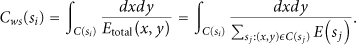
Figure 1 shows the changes in the total energy of the network (the sum of energy of the individual nodes) against time. As it is evident, the total energy of the network decreases linearly at first, but, after a certain point, it shows nonlinear behavior. Clearly, this phenomenon accelerates the depletion of network's energy. In order to find solution to eliminate this unwanted behavior, we first have to examine its possible reasons.

Figure 1

Total energy of the network against time.

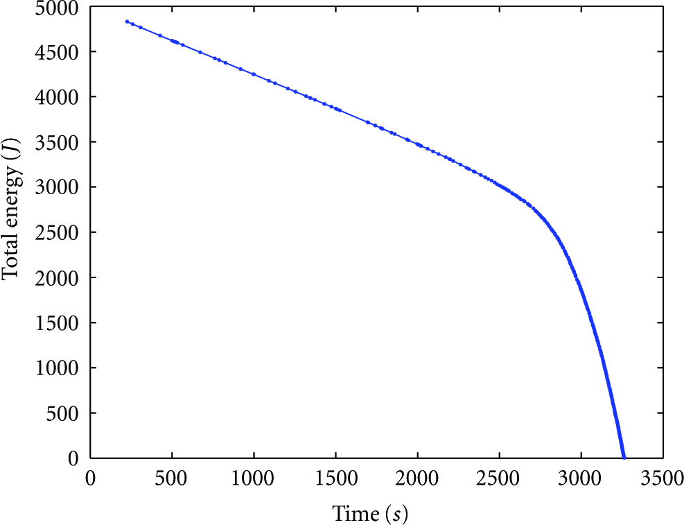
The node's energy is spent for various reasons such as communication, sensing, performing inside-node computations and so forth. Communication is the most energy consuming task in almost every application. The energy required to receive or transmit data for every node is modeled by the model introduced in [10]

$\begin{array}{c}Et\left(l,d\right)=\{\begin{array}{c}l\times E_{\text{elec}}+l\times {ϵ}_{\text{friss\_amp}}\times d^2\hfill \\ \hspace{1em}\hspace{1em}\hspace{1em}\hspace{1em}\hspace{1em}\hspace{1em}:d<d_{\text{cross-over}}\hfill \\ l\times E_{\text{elec}}+l\times {ϵ}_{\text{two\_ray\_amp}}\times d^4\hfill \\ \hspace{1em}\hspace{1em}\hspace{1em}\hspace{1em}\hspace{1em}\hspace{1em}:d>d_{\text{cross-over}},\hfill \end{array}\\ Er\left(l\right)=l\times E_{\text{elec}},\end{array}$

(2)

where $Et(l,d)$ is the energy required for a node to send l bits of data over a distance of d, and $Er(l)$ is the required energy to receive an l bit packet. $E_{\text{elec}}$ is consumed energy by electronic circuits and depends on factors such as digital coding, modulation, and so forth, ${ϵ}_{\text{friss\_amp}}$ and ${ϵ}_{\text{two\_ray\_amp}}$ are parameters dependent on the required receiver sensitivity and the receiver noise figure. $d_{\text{cross-over}}$ is the maximum distance of 2 nodes in order for them to have a direct line of sight thus, if a node sends a packet to a destination further than $d_{\text{cross-over}}$ , the transmission energy will be proportional to $d^4$ . Needless to say, this will increase the energy consumption rate of the node. This phenomenon would not affect the overall performance of the network in cases that the dimensions of monitored area are less than $d_{\text{cross-over}}$ . However, in larger areas, it can have serious impacts. In our setup, we consider a network with radio characteristics given in Table 1.

Table 1

Radio characteristics of the network.

Description	Parameter	Value
Cross over distance for Friss and two-ray ground attenuation models	$d_{\text{crossover}}$	$\frac{4\pi h_r{h}_t}{\lambda }$
Transmit power	$P_t$	${ϵ}_{\text{friss\_amp}}{R}_b{d}^2:d<d_{\text{crossover}}$    ${ϵ}_{\text{two\_ray\_amp}}{R}_b{d}^4:d\ge d_{\text{crossover}}$
Receive power	$P_r$	$\frac{{ϵ}_{\text{friss\_amp}}{R}_b{G}_t{G}_r{\lambda }^2}{{(4\pi )}^2}:d<d_{\text{crossover}}$    ${ϵ}_{\text{two\_ray\_amp}}{R}_b{G}_t{G}_r{h}_t^2{h}_r^2:d\ge d_{\text{crossover}}$
Minimum receiver power needed for successful reception	$P_{r\text{\_thresh}}$	6. 3 nW
Radio amplifier energy	${ϵ}_{\text{friss\_amp}}$ ${ϵ}_{\text{two\_ray\_amp}}$	$\frac{P_{r\text{\_thresh}}{(4\pi )}^2}{R_b{G}_t{G}_r{\lambda }^2}$    $\frac{P_{r\text{\_thresh}}}{R_b{G}_t{G}_r{h}_t^2{h}_r^2}$
Radio electronics energy	$E_{\text{elec}}$	50 nJ/bit
Compute energy for beamforming	$E_{\text{BF}}$	5 nJ/bit
Bitrate	$R_b$	1 Mbps
Antenna gain factor	$G_t{,\hspace{0.17em}\hspace{0.17em}G}_r$	1
Antenna height above the ground	$h_t{,\hspace{0.17em}\hspace{0.17em}h}_r$	1 m
Signal wavelength	λ	0. 325 m

According to the parameters given in Table 1, $d_{\text{cross-over}}$ would be 38. 31 [m]. We use a 400 × 400 [m²] area to observe the effect of $d_{\text{cross-over}}$ .

In this scenario, 1000 nodes are deployed randomly over a 400 × 400 [m²] area. The coverage of the network at its initial state is more that 97% which is a reasonable approximation of a fully covered network. For illustrative purposes, network lifetime is divided into some intervals with a length of 500 [s]. To get a better understanding of the pattern of energy consumption through time, we took a snapshot of the network after every interval.

As it is shown in Figure 2, energy consumption of the nodes is nonuniform and is dependent on their distance from the base station. The reason is that nodes closer to the base station carry a higher rate of traffic. To put it simply, CHs form multihop routes to send their data to the base station, and since according to (2) communicating over long distances is very energy consuming, the last hop of every multihop route would be elected among nodes located relatively close to the center in order to avoid long-distance communication to the base station. As a result, central nodes are used for communication purposes more often; therefore, they lose their energy faster. Obviously, this procedure cannot continue for a long time. Excessive use of central nodes leads to the formation of a low-energy and therefore high-cost area surrounding the base station. Due to the energy-aware characteristic of the algorithm, distant nodes gradually refuse to use these high-cost nodes as hops. The result is that distant nodes are compelled to send their data over longer distances, and according to (2), because $Et$ increases nonlinearly when d is increased (proportional to $d^2$ ), they lose their energy at higher rates. Moreover, if the distance becomes more than $d_{\text{cross-over}}$ , $Et$ will increase at excessive higher rates (proportional to $d^4$ ).

Figure 2

Snapshots of network after every 500 [s].

To take a more precise look, although central nodes carry a heavy load of traffic, nodes located extremely close to the center seem to be excluded from this problem. This fact is shown in Figure 3. According to Figure 3, we calculate the communication energy to send a bit of data from C to A from 2 different paths, and we show that if B is located extremely close to A, it would be better for C to communicate directly with A instead of using B as its interface.

Figure 3

Path1: C, A $E_{\text{total1}}=Et(\text{CA})+Er(\text{A})$ . Path2: C, B, A $E_{\text{total2}}=Et(\text{CB})+Er(\text{B})+Et(\text{BA})+Er(\text{A})$ . If $\text{BA}\to 0\Rightarrow \text{CA}\to \text{CB}$ ; $\text{BA}\to 0\Rightarrow E_{\text{total2}}>E_{\text{total1}}$ .

It seems that nodes extremely close to the base station are less probable to be elected as hops by CHs compared to those located somewhat further. In other words, in the early communication rounds, the percentage of nodes' participation in routing at first increases as we get closer to the center, but, after passing a certain point, it will start to decrease, so it seems to have a maximum at a certain distance from the base station. As discussed before, communication is the most energy-consuming task of the nodes, thus any change in the percentage of nodes' participation in routing would lead to similar changes in nodes' energy consumption, and therefore in their cost.

Taking all the facts into account, it seems that the critical, high-cost area formed around the base station is similar to a ring. These conclusions can be confirmed by the simulation results. Figure 4 shows the cost of nodes versus their distance from the base station after every 500 [s]. The figure shows that there is a peak in the node's cost at a certain point. Of course, the location of this peak is dependent on the assumed parameters of this simulation (Table 3). With our setup, the maximum cost occurs at about $d=50$  [m] which is a circle with the radius of 50 meters with its center located at the base station.

Figure 4

Cost of nodes against their distance from the base station after every 500 [s].

5. The Proposed Solution

According to Figure 4, the formation of a high-cost ring causes long-distance communications and leads to inefficient energy consumption. This problem can be solved by modifying the distribution of nodes. Since nodes in the critical ring are more often used and therefore are more important compared to other nodes, a distribution with higher concentration of nodes in the critical areas seems to be more proper than a uniform distribution. By taking a deeper look into Figure 4, we can see that cost of nodes is a function of their distance from center. We can also recognize a pattern similar to gamma distribution (explained in (3)). The pattern formed in the cost of nodes over time is a measure of their importance in routing or in other words their potential for early depletion. In order to neutralize this effect, we tend to choose a nonlinear distribution that distributes energy in the network with the same pattern seen in Figure 4. In this way, areas that are more probable to be depleted of energy are provided with more initial energy proportionally. Therefore, we suggest gamma distribution for distributing nodes (see Figure 5).

Figure 5

Gamma distribution.

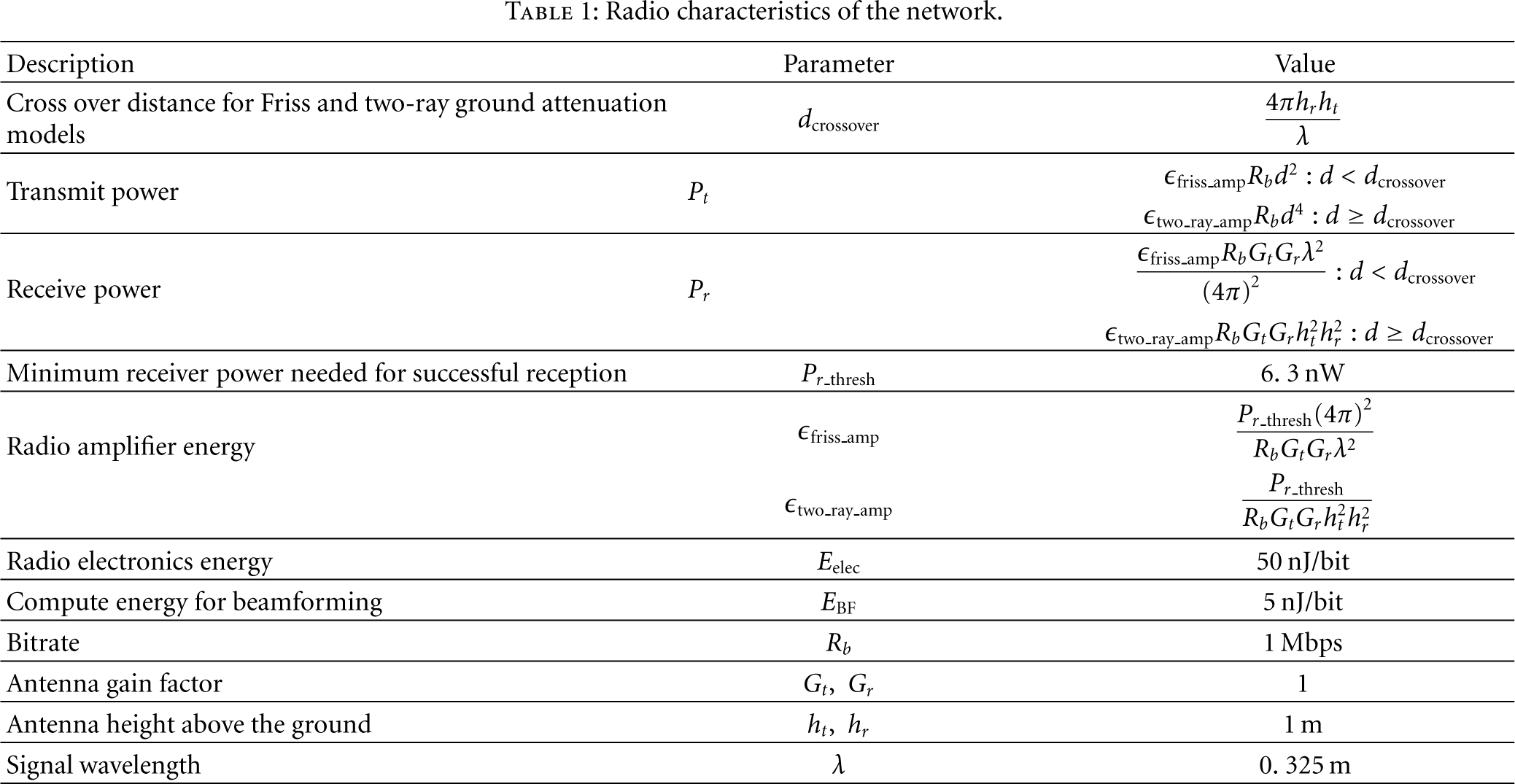
However, a paramount factor that should be taken into consideration is that the number of nodes is constant at 1000 nodes. Therefore, existence of certain densely populated areas will cause other areas to be sparsely covered. This fact will limit the degree to which we can concentrate nodes at the critical area. To put it simply, we have to make sure that the network has a high coverage percentage at its initial state (more than 97%); therefore, there cannot be an unlimited increase in the density of nodes in some areas. To solve this problem, we propose a compromise. We divide the nodes into two groups. We first distribute $N1$ nodes randomly in the area, and then we deploy the remaining $1000-N1$ nodes using a gamma distribution as explained below.

$\begin{array}{c}y=f\left(x\hspace{0.17em}|\hspace{0.17em}a,b\right)=\hspace{0.17em}\hspace{0.17em}\frac{1}{b^a\Gamma \left(\text{a}\right)}{x}^{a-1}{e}^{-x/b},\hspace{1em}\left(a=1.5,\hspace{0.17em}\hspace{0.17em}b=100\right).\end{array}$

(3)

In fact, we place $1000-N1$ nodes in $(r,\theta )$ positions. Where r is determined according to (3) and θ is chosen uniformly. Our goal to guarantee the initial coverage tends to increase $N1$ whereas our objective to concentrate nodes on the critical ring tends to increase $1000-N1$ and consequently decrease $N1$ . A compromise must be made. We try to decline $N1$ to the minimum point possible that the initial coverage remains more than 97%. Table 2 shows the average initial coverage obtained by MATLAB simulation for different values of $N1$ . According to Table 2, $N1=600$ is a reasonable choice to keep the initial coverage percentage over 97%.

Table 2

Average initial coverage of network for different values of $N1$ .

Number of nodes deployed randomly ( $N1$ )	Number of nodes deployed with gamma distribution ( $1000-N1$ )	Average initial coverage (%)
400	600	94.13
500	500	95.76
600	400	97.29

Table 3

Simulation parameters.

Parameter	Value
Number of nodes	1000
Initial energy of each node	5 [J]
Dimensions of monitored area	400 × 400 [m2]
$E_{\text{elec}}$	50 [nJ/bit]
${ϵ}_{\text{friss\_amp}}$	10 [pJ/bit/m2]
${ϵ}_{two\text{\_ray\_amp}}$	0. 0066 [pJ/bit/m4]
$d_{\text{cross-over}}$	38.31 [m]
Packet rate	1 [packet/s]
$R_{\text{sense}}$	15 [m]

6. Simulation Results

We used the parameters indicated in Table 3 and our proposed nonuniform distribution. Figure 6 shows snapshots of the network after every 500 [s]. A comparison of Figures 6 and 2 will give us more insight into the network's operation over time. In uniform distribution scenario (Figure 2), the formation of a high-cost region around the base station initiating from early communication rounds is clearly observable. In Figure 2(d), which corresponds to $t=2000$  [s], we can identify the mentioned area that develops by time as is illustrated in succeeding figures. However, network with our nonuniform distribution shows a more homogeneous behavior in sense of energy consumption. In Figure 6(h), which corresponds to a time approximately equivalent to the lifetime of the network with uniform distribution, the critical area has not been shaped yet resulting in the linear behavior of the network. Although we could not totally eliminate the formation of critical area, (due to the limitations imposed by the coverage-preserving requirements and limited number of nodes), we could greatly delay this event to reduce the nonlinearity of network.

Figure 6

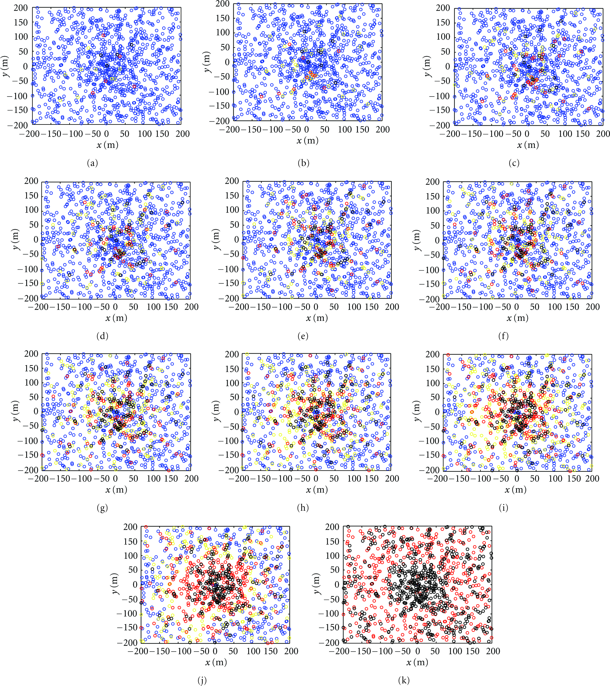
Snapshots of network with our proposed distribution after every 500 [s].

Figure 7 shows the cost of nodes against their distance from center after every 500 [s]. Our effort to guaranty the homogeneous energy consumption over time translates into equalizing the cost of nodes located in various distances from the center during the network lifetime. By contrasting Figure 7 with Figure 4, we will observe the removal of the peak shaped in Figure 4 when the nonuniform distribution is applied. Due to the limitations discussed above, cost of nodes cannot be completely equal. However, its variation is substantially reduced.

Figure 7

Cost of nodes against their distance from the base station after every 500 [s] in a network with our proposed distribution.

Finally, Figure 8 shows changes in the total energy of the network over time using our method for distributing nodes in comparison with the uniform distribution. As it is illustrated, when using nonuniform distribution, the network remains its linear behavior for a longer period, so we expect a longer lifetime for the network. Theoretically, nonlinear behavior of the system emerges as soon as the formation of a high-cost corona that obliges forwarding packets to skip it during routing. Our approach in this paper was to find the most vulnerable area to energy depletion and make this area robust by concentrating more nodes and therefore more energy there. With a constant number of nodes and having in mind our obligation to satisfy the initial coverage threshold, we are confined to a predetermined number of nodes to deploy in critical regions. Therefore, although we can postpone the initiation of nonlinearity, we might not be able to completely eliminate it. In other words, we tend to make the critical region as robust as possible compared to the uniform distribution, but, considering the high traffic rate of this area, we cannot guaranty linear behavior throughout the whole lifetime.

Figure 8

Energy consumption of network using the proposed nonuniform distribution [red] compared to the uniform distribution [blue].

Figure 9 shows the coverage of network against time for both distributions. Using this figure, we can get a clear understanding of the improvement made in network's lifetime. As defined earlier, lifetime of the network is the amount of time that the coverage is more than 90%. According to Figure 9, a 66% improvement of the lifetime has occurred using the proposed distribution.

Figure 9

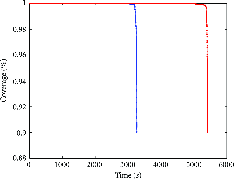
Coverage against time using the proposed nonuniform distribution [red] compared to the uniform distribution [blue].

7. Conclusion

In this paper, we studied the relation between nodes' location and their energy consumption in a wireless sensor network during the network's lifetime. We showed that the uniform distribution of nodes in the monitored area leads to inefficient use of energy resources. To find better distribution scenarios, we located critical areas in the network. Then, we proposed a proper solution that concentrates nodes on critical areas to the highest degree that is possible in order for the network to maintain its initial coverage more than a reasonable threshold. Using this scenario, we demonstrated the progress made in the lifetime by simulation results.