A Top-Down Clustering and Cluster-Tree-Based Routing Scheme for Wireless Sensor Networks

Abstract

Cluster-based organization of large sensor networks is the basis for many techniques aimed at enhancing power conservation and network management. A backbone network in the form of a cluster tree further enhances routing, broadcasting, and in-network processing. We propose a configurable top-down cluster and cluster-tree formation algorithm, a cluster-tree self-optimization phase, a hierarchical cluster addressing scheme, and a routing scheme. Such self-organization makes it possible to effectively deliver messages to a sink as well as within the network. For example, a circular sensor field with a sink in the center can establish cross-links and circular-paths within the cluster tree to deliver messages through shorter routes while reducing hotspots and consequently increasing network lifetime. Cluster and cluster-tree formation algorithm is independent of physical topology, and does not require a priori neighborhood information, location awareness, or time synchronization. Algorithm parameters allow for formation of cluster trees with desirable properties such as controlled breadth/depth, uniform cluster size, and circular clusters. Characteristics of clusters, cluster tree, and routing are used to demonstrate the effectiveness of the schemes over existing techniques.

1. Introduction

Advances in wireless communications and miniature, low-power, and low-cost sensors are enabling the deployment of large-scale and collaborative wireless sensor networks (WSNs). These networks enhance our perception of the surroundings by sensing the physical world at far greater temporal and spatial granularities than been hitherto possible. Numerous WSN systems are being proposed and implemented leading to novel applications in areas such as habitat monitoring, disaster response, eldercare, and battlefield intelligence.

Energy-efficient operation, channel contention, latency, and management of WSNs are complex and critical issues that have to be addressed to facilitate large-scale deployments. Cluster-based organization of large sensor networks is the basis for many techniques that address these issues [1–13]. Applications that span large sensor fields and/or support data aggregation are prime candidates for cluster-based configuration. Clustering is particularly useful in collaborative sensor applications that perform different tasks and deployed in the same physical area [14]. In general, the network is decomposed into a set of clusters, for example, for administrative or communicating purposes, with each cluster formed by grouping a set of nearby nodes. A designated node, namely, the cluster head (CH), manages each cluster. With many solutions based on clustering, the nodes within a cluster communicate only with their CH. The CHs are responsible for coordinating both intercluster and intracluster communication. Communication among CHs can be via either single or multiple hops.

Cluster formation can be either distributed or centralized. Many distributed clustering solutions including [1–4] achieve longer network lifetime by selecting CHs based on residual energy of nodes. LEACH-C [1] is a centralized solution that further enhances the network lifetime. Typically, overhead of local knowledge-based distributed clustering solutions is lower compared to that of centralized solutions such as LEACH-C. However, their lack of global knowledge limits the possibility of forming an optimum set of clusters, that is, fails to achieve maximum spatial coverage with least number of clusters. Even with the presence of such information, selecting a minimum set of clusters with maximum coverage is an NP-hard problem [15]. Hybrid schemes that combine local and neighbors' view of the topology can form better clusters while having low overhead [5]. For example, ACE [6] and FLOC [7] form more uniform and circular clusters. Solutions in [1–3, 6–8] assume all CHs are capable of directly communicating with the sink. This may not be possible in a geographically large network where the sink is beyond the transmission range of many nodes.

Though many clustering solutions have been proposed [16], only a few combines clustering with a data routing scheme that is appropriate for large-scale WSNs [9–12, 17]. Hierarchical topologies are attractive for such large networks because of the scalability. A backbone network that arranges CHs in the form of a cluster tree can facilitate both the node-to-sink and node-to-node communication. Cluster trees are useful for a multitude of tasks such as delivering unicast, multicast, and broadcast traffic, data fusion, and in-network query processing.

A cluster tree can be formed using either a top-down or a bottom-up approach. In top-down approach, a designated root node first forms its own cluster. It then selects some of its neighbors (as CHs) to form their own clusters, which in turn causes some of their neighbors to form the next level of clusters, and the process continues until the entire sensor field is covered. The cluster tree is formed by keeping track of the parent-child relationship among CHs, and it is guaranteed to be connected as new child CHs are selected from neighbors of existing CHs. The IEEE 802.15.4 cluster tree follows this concept [18].

In bottom-up approach, individual clusters are formed independently and later combined together to form a higher-level structure. In [9], for example, nodes probabilistically elect themselves as CHs at different levels of the hierarchy and form their own clusters. The hierarchy is then formed by directly connecting a set of CHs at level i to a CH at level $i+1$ . TEEN [10] follows a similar concept. The physical distance between CHs of adjacent levels increases as we go up the hierarchy [19]. Thus, upper level CHs become hotspots, as they have to relay traffic from lower layers and require higher transmission energy levels. Power balanced unequal cluster formation [4, 12, 16] overcomes this issue by forming many smaller clusters closer to the sink and making them larger as the distance to the sink increases. However, clusters are more likely to become arbitrarily large the further they are from the sink. Therefore, schemes in [4, 9, 10, 12, 16] cannot guarantee CH-to-CH connectivity in geographically large networks because the intercluster distance is not bounded. An alternative would be to use gateway nodes [17] or reposition CHs [11]. ZigBee standard [17] proposes an alternative scheme for clustering IEEE 802.15.4 networks [18]. It first forms an independent set of clusters and later combines them into a cluster tree through gateway nodes. In [11], a set of CHs is selected to form an independent dominating set. Some of those CHs are later repositioned to obtain connectivity. However, CH repositioning is costly and could deteriorate desirable properties of independent dominating sets.

The bottom-up approach, although conceptually appears to be relatively simple, involves considerable communication overhead for building a cluster tree [8–10, 17], and it provides very little or no control over depth and breadth of the tree. Conceptually, the top-down approach provides better control while forming clusters and the cluster tree. However, the existing top-down approaches, such as the basic scheme for IEEE 802.15.4 standard, result in undesirable cluster and tree characteristics such as large variations in cluster size and distance to leaf nodes [5, 13]. Within the framework of the IEEE 802.15.4 standard, however, there is flexibility to deploy alternative clustering approaches while still being compatible with the standard. We propose a configurable top-down clustering scheme in which parameters such as the number of nodes in a cluster and the breadth/depth of the cluster tree can be easily controlled while maintaining compatibility with the IEEE 802.15.4 standard.

A good clustering and routing solution should achieve the following desirable properties. Overlapping clusters add redundancy [20] and increase intracluster signal contention [2]. Thus, a given sensor field should be covered with the least number of clusters. Hexagonal clusters have the highest coverage area and cover the network with the least number of clusters [6, 20]. None-overlapping clusters allow better load balancing within clusters, bound the number of clusters and depth of the cluster tree tighter, and generate networks with predictable topology characteristics [6, 7]. Predictable topology characteristics, even on a randomly deployed network, facilitate intelligent routing solutions without being tied to the cluster tree. Aggregation is more useful when the CH is in the center of the cluster and capable of receiving sensor readings from all the directions [7]. Performance of upper layer functions such as routing and data fusion depend on the number of hops between nodes and the sink. As the hop count increases, both latency and energy required to forward a message increase. Therefore, a lower depth cluster tree is desirable. Less overlapped clusters also reduce the breadth and depth of the cluster tree [13]. Furthermore, distance between two adjacent CHs needs to be bounded to ensure the connectivity of the cluster tree. In summary, a good clustering solution should form clusters with minimum overlap, minimize the depth of the cluster tree, and ensure connectivity.

We propose a compound solution that achieves the aforementioned desirable cluster and cluster-tree properties while enabling efficient communication within large-scale WSNs. First, we propose the generic top-down cluster and cluster-tree formation (GTC) algorithm. GTC achieves desirable cluster and cluster-tree properties by combining the controllability of the top-down approach with local and neighbors' views of the topology. The algorithm is independent of the physical network topology and does not require a priori neighborhood information, location awareness, or time synchronization. Parameters in the algorithm allow cluster and tree characteristics to be changed, for example, a tree with controlled breadth/depth, while achieving more uniform and circular clusters. The IEEE 802.15.4 cluster tree [18], hereafter referred to as simple hierarchical clustering (SHC), is a special case of GTC achievable by controlling algorithmic parameters. Another special case, hop-ahead hierarchical clustering (HHC), is presented that produces more circular and uniform clusters and a cluster tree with lower depth. Cluster properties of HHC are comparable with hexagonal packing, particularly for low-density networks. The cluster tree is guaranteed to be connected as GTC bounds the distance between a parent and its child CHs. Second, we propose a post cluster-tree self-optimization phase that further enhances the structure of the cluster-tree, reduces its depth, and improves routability. Third, a hierarchical addressing scheme that reflects the parent-child relationship among CHs is proposed. Such hierarchical addresses simplify routing and help to reduce the size of routing tables. Fourth, a cluster-tree-based routing scheme that can forward messages to the sink as well as within the network is presented. Two routing extensions, namely cross-link-based routing and circular-path-based routing, are presented, that deliver more than two, and five-times more messages, respectively. These routing schemes enable multiple and shorter routes to a given destination.

Section 2 presents the GTC algorithm, controlling the cluster and cluster tree properties, and the self-optimization phase. Hierarchical addressing and routing schemes are presented in Section 3. Section 4 presents the performance analysis. Concluding remarks and future work are presented in Section 5.

2. Cluster and Cluster Tree Formation

2.1. Top-Down Clustering Algorithm

A discussion of basic algorithm steps is presented first, followed by the specific details. The root node, one of the sensor nodes or a resourceful base station, initiates the cluster formation process by sending a broadcast indicating its interest to form a cluster. Nodes that hear the broadcast become members of the cluster by sending an acknowledgment (ACK) to the root node. Coverage of a cluster depends on whether a single-hop or a multihop cluster is formed by forwarding the broadcast through neighbors. The parameter hops_max is used to provide a bound on the number of hops to a cluster member from the CH. After receiving ACKs from neighbors, the root node selects several new child CHs from subset of the nodes closer to the cluster boundary. Overlap among clusters can be reduced by selecting child CHs from nodes that are outside the cluster boundary. Such outside nodes can be discovered by forwarding the broadcast beyond hops_max and their distance can be bound using the parameter TTL_max (TTL_max ≥ hops_max). The root node then requests those selected child CHs to form their own clusters in turn by sending a unicast message to each of them. New CHs form their own clusters and then select the next set of child CHs and the process continues. Meanwhile, the cluster tree is formed by each CH keeping track of its parent and child CHs. The algorithm continues until all the possible clusters are formed.

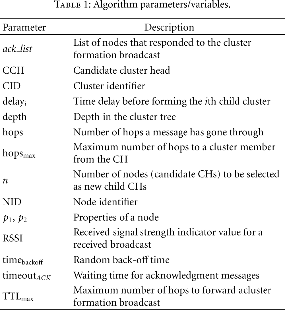
The Generic Top-down Cluster and cluster-tree formation (GTC) algorithm is shown in Algorithm 1. The root node initiates the cluster formation process by executing the Form_Cluster function. All the other nodes execute the Join_Cluster function and listen for a cluster-formation broadcast. Root node sends a cluster-formation broadcast (Bcast_Cluster) indicating its node ID (NID_CH), Cluster ID (CID_CH), maximum number of hops to a cluster member from the CH (hops_max), number of hops to forward the broadcast (TTL_max), and its depth in the cluster tree. Important algorithm parameters are listed in Table 1. A node hearing this broadcast will join the cluster, if it is not already a member of another cluster (my_CID = 0) and within hops_max. A node joins the cluster by initializing its cluster parameters such as cluster ID, CH's node ID, and depth in the cluster tree (lines 17–19, Algorithm 1). An acknowledgment (ACK) is then sent to the corresponding CH (line 20) indicating its own node ID (my_NID), distance to the CH (hops), and set of properties of the node ( $p_1,p_2$ ) such as residual energy and node degree. The CH receiving the ACK adds the sender to its list of acknowledged nodes (ack_list). After sending the ACK, the node waits a random back-off time (line 22), and then forwards the cluster-formation broadcast (Fwd_Bcast_Cluster), if TTL is still valid. Random back-off time helps to reduce collisions among transmitting nodes.

Table 1

Algorithm parameters/variables.

Parameter	Description
ack_list	List of nodes that responded to the cluster formation broadcast
CCH	Candidate cluster head
CID	Cluster identifier
delayi	Time delay before forming the ith child cluster
depth	Depth in the cluster tree
hops	Number of hops a message has gone through
hopsmax	Maximum number of hops to a cluster member from the CH
n	Number of nodes (candidate CHs) to be selected as new child CHs
NID	Node identifier
$p_1$ , $p_2$	Properties of a node
RSSI	Received signal strength indicator value for a received broadcast
timebackoff	Random back-off time
timeoutACK	Waiting time for acknowledgment messages
TTLmax	Maximum number of hops to forward acluster formation broadcast

Algorithm 1: The generic top-down cluster and cluster-tree formation algorithm.

    Form_Cluster (NID _CH , CID _CH , delay, n , hops _max , TTL _max , depth)

 (1) Wait (delay)

 (2)  $TTL\leftarrow {TTL}_{\max \hspace{0.17em}}$

 (3) Bcast_Cluster ( ${NID}_{CH}$ , ${CID}_{CH}$ , ${hops}_{\max \hspace{0.17em}}$ , ${TTL}_{\max \hspace{0.17em}}$ , $TTL$ , depth)

 (4) ack_list ←Receive_ACK ( ${NID}_{child}$ , $hops$ , $p_1$ , $p_2$ , ${timeout}_{ACK}$ )

 (5)  IF (ack_list = NULL)

 (6)   Join_Cluster()

 (7) FOR   $i=1$    TO    $n$

 (8)     ${CCH}_i\leftarrow$ Select_Child_CHs (ack_list)

 (9)     ${CID}_i\leftarrow$ Select_Next_ $CID\hspace{0.17em}\hspace{0.17em}(i)$

 (10)   delay_i← Select_Delay $(i)$

 (11)   depth_i← depth + 1

 (12)   Rqst_Form_Cluster ( ${CCH}_i$ , ${CID}_i$ , delay_i, n, ${hops}_{\max \hspace{0.17em}}$ , ${TTL}_{\max \hspace{0.17em}}$ , depth_i)

    Join_cluster()

 (13) Lstn_Bcast_Cluster ( ${NID}_{CH}$ , CID_CH, ${hops}_{\max \hspace{0.17em}}$ , ${TTL}_{\max \hspace{0.17em}}$ , $TTL$ , depth)

 (14)  $TTL\leftarrow TTL-1$

 (15)  $hops\leftarrow {TTL}_{\max \hspace{0.17em}}-TTL$

 (16) IF ( $hops\le {hops}_{\max \hspace{0.17em}}\hspace{0.17em}\hspace{0.17em}\mathbf{A}\mathbf{N}\mathbf{D}\hspace{0.17em}\hspace{0.17em}my\_CID=0$ )

 (17)    $my\_CID\leftarrow {CID}_{CH}$

 (18)    $my\_CH\leftarrow {NID}_{CH}$

 (19)    $my\_depth\leftarrow depth+1$

 (20)   Send_ACK (my_NID, hops, $p_1$ , $p_2$ )

 (21) IF ( $TTL\hspace{0.17em}\hspace{0.17em}>\hspace{0.17em}\hspace{0.17em}0$ )

 (22)    Wait (Random (time_backoff))

 (23)    Fwd_Bcast_Cluster ( ${NID}_{CH}$ , ${CID}_{CH}$ , ${hops}_{\max \hspace{0.17em}}$ , ${TTL}_{\max \hspace{0.17em}}$ , $TTL$ , depth)

 (24)    IF ( $hops\le {hops}_{\max \hspace{0.17em}}$ )

 (25)      Exit $()$

 (26) ELSE

 (27)    IF (Wait_Lstn_Neighbors (Random(time_backoff))= FALSE)

 (28)      Send_ACK(my_NID, hops, $p_1$ , $p_2$ )

 (29)      IF (Lstn_Form_Cluster( $CCH$ , $CID$ , delay, n, ${hops}_{\max \hspace{0.17em}}$ , ${TTL}_{\max \hspace{0.17em}}$ , depth, ${timeout}_{CCH}$ ) = TRUE )

 (30)         Form_Cluster (my_NID, CID, delay, n, ${hops}_{\max \hspace{0.17em}}$ , ${TTL}_{\max \hspace{0.17em}}$ , depth)

 (31)         Exit $()$

 (32) Join_cluster $()$

Intermediate nodes between (hops_max, TTL_max) hops do not join the cluster, instead help forward the broadcast further. They do not send any ACKs. A broadcast from a particular CH is forwarded only once by a receiving node; hence, broadcasts are forwarded outward from the CH. When the broadcast reaches the last hop (i.e., TTL expires) the nodes that received the broadcast are capable of being selected as new CHs. Such a node is called a candidate cluster head (CCH). At this stage, the CCH nodes are either at the edge of the cluster (if TTL_max = hops_max) or outside the cluster (if TTL_max > hops_max). By listening to the transmissions from neighbors, the possibility of selecting two nearby nodes as CCHs can be reduced. Therefore, each candidate node waits a random time (Wait_Lstn_Neighbors) before sending an ACK to the corresponding CH. While waiting, nodes keep listening and try to detect any ACKs sent by their neighbors to the same CH. If such an ACK is detected (line 27, function returns TRUE), the node gives up its candidacy to be a new CH and retries to join a cluster, that is, reruns the Join_Cluster function. If no ACK is detected by the time the function timeouts (no neighbor is still interested in becoming a CCH), node confirms itself as a CCH and informs this to the corresponding CH by sending an ACK (line 28). Child CHs are chosen from this spatially distributed set of CCHs, and therefore generates a less overlapping set of clusters. After sending the ACK, each CCH waits for a cluster formation request (Lstn_Form_Cluster) from the corresponding CH. Meanwhile, a CCH may join a different cluster if it hears a new broadcast and is within hops_max from the new CH. This further prevents the formation of overlapping clusters and ensures all nodes are covered by clusters.

In the meantime, the corresponding CH keeps receiving ACKs until the Receive_ACK function timeouts (line 4). A new set of child CHs are then selected from the CCHs in the ack_list, using the Select_Child_CHs function. Finally, a request is sent to each selected CCH asking them to form their own clusters (Rqst_Form_Cluster). Each request also includes the new cluster's ID (CID _i ), a hold-up time (delay _i ) before forming the new cluster, and other relevant parameters. Upon receiving the requests, selected CCHs form their own clusters by executing the Form_Cluster function. These CHs then select the next set of child CHs and the process continues. The cluster tree is rooted at the root node and formed by each CH keeping track of its parent and child CHs. If a selected CCH is unable to attract any child nodes, a cluster is not formed and the related branch in the cluster tree is not expanded further. The algorithm continues until all possible branches are expanded.

2.2. Control of Clusters and Cluster Tree Characteristics

GTC algorithm can achieve a wide range of solutions by varying the implementation of functions Select_Child_CHs and Select_Delay, and controlling the parameters hops_max and TTL_max. hops_max controls the coverage of a cluster while TTL_max controls the distance between a parent and its child CHs. Multihop clusters are formed when hops_max > 1. When TTL_max = hops_max, CCHs are selected from nodes that are at the edge of the parent cluster. Figure 1(a) illustrates the best theoretical cluster packing that can be achieved when hops_max = TTL_max = 1. For simplicity, only a selected set of CCHs is shown and one branch is expanded into several levels. It is sufficient for a CH to select three CCHs, if those are separated physically as widely as possible. Let $n_i$ denote node i and $c_i$ denote cluster i. The root node ( $n_1$ ) forms cluster $c_1$ by connecting all one-hop neighbors. It then requests three of its neighbors $n_2$ , $n_3$ , and $n_4$ that are at the edge of the cluster, to form their own clusters $c_2$ , $c_3$ , and $c_4$ . How those three neighbors can be selected is addressed later. They are called level 1 clusters while the root node belongs to level 0. Then $n_2$ requests $n_5$ , $n_6$ , and $n_7$ to form their own clusters. Even in this conceptual case, the shapes of clusters are not circular except for $c_1$ . Many overlapped clusters are formed as we go down the tree. As the effective coverage of a cluster is small, many clusters and a longer cluster tree are required to cover the sensor field. This approach reflects the basic scheme proposed in the IEEE 802.15.4 standard and hereafter referred to as simple hierarchical clustering (SHC).

Figure 1

Physical shape of ideal single hop clusters: (a) simple hierarchical clustering, hops_max = TTL_max = 1; (b) hop-ahead hierarchical clustering, hops_max = 1, TTL_max = 3. Straight lines indicate the parent-child relationship among CHs.

The overlap between parent and child clusters can be reduced by selecting nodes that are outside the parent cluster as CCHs. Cluster-formation broadcasts can be propagated beyond the parent cluster (i.e., TTL_max > hops_max) through a set of intermediate nodes to select some of the distant nodes as CCHs. When TTL_max = 2hops_max, the overlap between a parent and its child clusters is reduced. It also ensures that both clusters have the same hop count. Though this is a significant improvement over SHC, clusters can still overlap due to random node placement, that is, it is not always possible to find an optimum set of CCHs that is furthest from the parent CH. For minimum overlap, the ideal distance between a CH and its CCHs should be just above 2hops_max. Hence, it is more appropriate to select TTL_max = 2hops_max + 1. This multihop forwarding approach is named hop-ahead hierarchical clustering (HHC). Figure 1(b) illustrates the ideal circular packing with single-hop HHC. The root node ( $n_1$ ) sends a cluster-formation broadcast and all one-hop neighbors join $c_1$ . The broadcast is then forwarded until TTL expires. For example, after hearing the broadcast from $n_1$ , $n_2$ joins the cluster. The broadcast is then forwarded from $n_2$ to $n_3$ and from $n_3$ to $n_4$ . Finally, $n_4$ is three-hops away from the CH, and hence it becomes a CCH. The root node selects six such nodes ( $n_4$ to $n_9$ ) that are in different directions of the sensor field as child CHs. Different mechanisms that can be used to select those six nodes are discussed later. For all the other levels it is sufficient that each parent CH selects up to three nodes as child CHs, for example, $c_8$ , $c_9$ , and $c_{10}$ are formed by $c_4$ . Due to this setup, HHC scheme forms larger clusters, more circular clusters, and has a better distribution of CHs.

Each parent CH uses the Select_Child_CHs function to select child CHs from a set of CCHs. Implementation of the function depends on the availability of node properties such as node degree, residual energy, cryptographic key identifiers, or location information. When a node sends an ACK to the CH, such properties are reported using parameters $p_1$ and $p_2$ . Load balancing can be achieved by selecting CCHs based on higher residual energy or lower node degree [2]. If the cluster setup phase is cycled like in [1, 2], such parameters play a key role in selecting different sets of CHs in different cycles. In [21], we illustrate the use of GTC algorithm with predistributed cryptographic key identifiers to build a secure backbone. Node location information is essential to select a precise set of child CHs. However, due to constraints on cost, size, energy consumption, and implementation environment, most sensor nodes are not location aware [22]. The received signal strength indicator (RSSI), available in most wireless devices, can be used to estimate the distance between two nodes. RSSI is attractive because it has minimum impact on hardware, power consumption, and cost. Though RSSI is not very reliable, it has been demonstrated that RSSI measurements in new radios such as CC2420 [23] are stable over time [24, 25] and tend to decrease exponentially with the distance [24]. As cluster formation does not need highly accurate distance information, rather relative distance relationships between neighboring nodes, RSSI can serve as a reasonable first-order approximation needed for the relative distance values.

An RSSI-based heuristic to select a spatially distributed set of CCHs is presented next. Clusters overlap if CCHs are pushed by 2hops_max, but coverage holes are created if they are pushed all the way up to 2hops_max + 1 (Figure 1(b)). A better alternative would be to select a node that is just above 2hops_max as a CCH [13]. An RSSI-based heuristic can be used to forward the cluster-formation broadcast to the maximum distance within 2hops_max and then select a nearby node as a CCH. The heuristic can be implemented by modifying lines 22 and 27 of the GTC algorithm:

• (22)

Wait (RSSI + Random (time_backoff))

(27)

IF   (Wait_Lstn_Neighbors  (1/RSSI  +  Random (time_backoff)) = FALSE)

The waiting time now depends on the RSSI value of the received broadcast and the random back-off time. Random back-off time is used to differentiate the waiting time among nodes with the same RSSI. According to line 22, a node with a lower RSSI (i.e., higher distance) gets priority in forwarding the broadcast than a node with a higher RSSI. This allows the nodes that are furthest away from the CH and within 2hops_max to forward the broadcast first. Then in the last hop, a nearby node (i.e., one with higher RSSI; note 1/RSSI in line 27) gets priority in becoming a CCH than a distant node. Therefore, the time that such a node keeps listening for ACKs (sent by neighbors) is shorter than the nodes that are further away. If such an ACK is detected, the node gives up its candidacy to be a new CH and retries to join a cluster. Thus, the waiting time is used to prevent nodes in the same neighborhood from becoming CCHs and thereby achieve spatial separation. Distant nodes are selected only if they do not hear any ACKs from their neighbors. Consequently, CCHs are primarily selected from a spatially separated set of nodes that are just beyond 2hops_max. Then n ( $n=6$ for first round of HHC, and $n=3$ otherwise) CCHs are randomly selected as child CHs. As the set of CCHs is spatially separated, child CHs selected from that set are also spatially separated. The RSSI based heuristic minimizes coverage holes, produces more uniform clusters, and reduces depth of the cluster tree. If no location information or RSSI is available, child CHs can still be selected randomly from the set of CCHs.

Cluster properties are affected when multiple child CHs try to form clusters at the same time. Therefore, we reduce collisions among cluster-formation broadcasts by a randomized scheduling scheme. Each parent CH determines a time delay (delay _i ) that each of its child CHs needs to wait before forming its own cluster, using the Select_Delay function. Furthermore, the shape of cluster tree can be controlled by appropriately selecting delay _i values. For breadth-first tree formation, delay should ensure that cluster formation of level j completes before the start of level $j+1$ . Thus, a parent CH can estimate when its first child CH should form the cluster using [13]:

$\begin{array}{c}{t}_j=j{t}_{\text{CH}}+\left(j-1\right)\left(n-1\right)t_{\text{CCH}},\end{array}$

(1)

where j is the child CHs level in cluster tree, $t_{\text{CH}}$ is the time required to form a cluster, $t_{\text{CCH}}$ ( $t_{\text{CCH}}\ge t_{\text{CH}}$ ) is the scheduled delay between formation of two child clusters of the same parent, and n is the number of child CHs (i.e., branching factor of the tree). Each of the remaining child clusters needs to be delayed by $t_{\text{CCH}}$ . Depth-first tree formation can be facilitated by allowing a branch to complete its expansion before start of another branch by the root node. This approach forms a longer tree that provides more opportunities for data aggregation. However, a longer tree increases latency and energy consumption therefore may not be desirable in many applications. Note that waiting time is just a delay, and thus the algorithm does not require time synchronization.

The cluster tree starts from the root node and is formed by each CH keeping track of its parent and child CHs. Parent and child CHs can be physically linked using either single-hop (high-power) or multihop (low-power) transmissions. Typically, long-range intercluster communication is desirable due to low latency and simplified routing [11, 16]. It further enables non-CHs to sleep while not sensing or transmitting [16]. Because any node is capable of becoming a CH, this approach is suitable if either the nodes can tune their transmission power or the CHs are later replaced by energy-rich actor nodes [11]. Henceforth, we assume high-power transmissions among CHs.

In top-down clustering, a set of child CHs is always selected from the nodes that are at a bounded distance from the parent CH. The cluster tree that connects those CHs is therefore guaranteed to be connected, if the intercluster communication range of CHs is higher than the distance bound. The same property holds for the GTC algorithm as the distance between a parent and its child CHs is bounded by TTL_max. Thus, the cluster tree is guaranteed to be connected if $R\ge r\times {\text{TTL}}_{\max \hspace{0.17em}}$ , where R and r are the intercluster and intracluster transmission ranges, respectively. Hence, GTC algorithm guarantees a connected topology compared to [1, 2, 9, 10] and does not require CH repositioning as in [11].

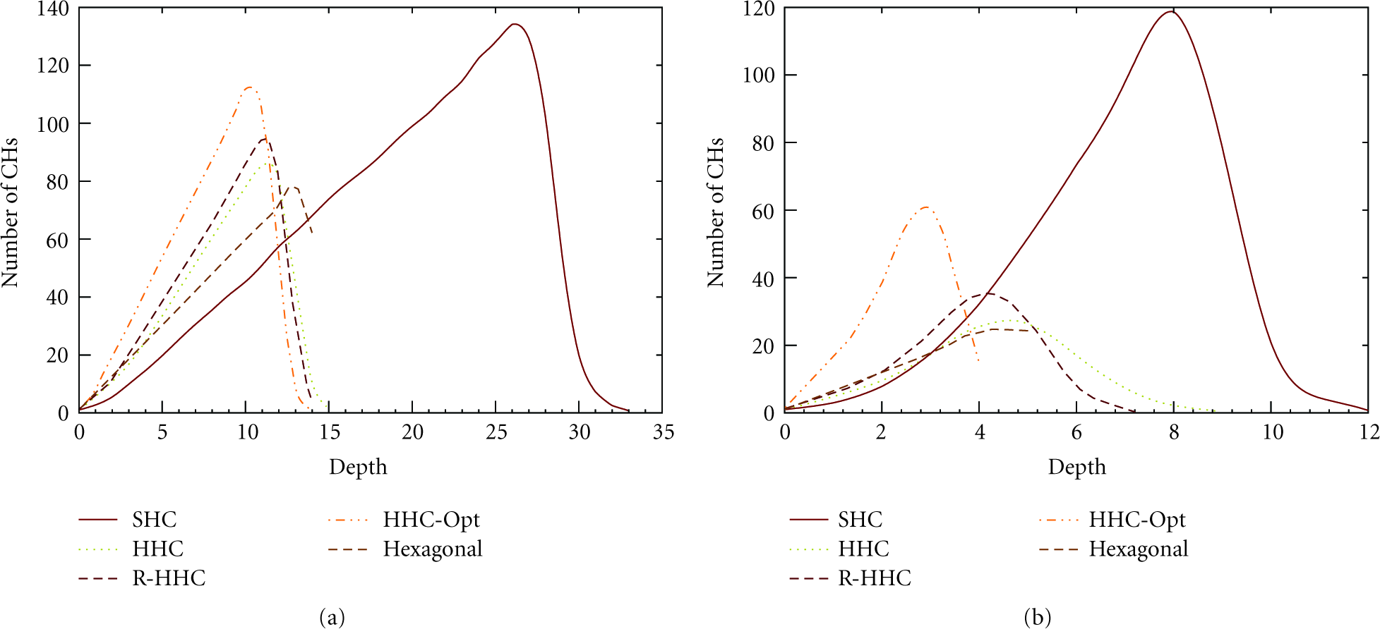
Based on hexagonal packing, lower and upper bounds are derived for the depth of a cluster tree formed by interconnecting single-hop clusters. Assume a circular sensor field (see Figure 2) with uniform node distribution. The root node is placed in the center of the sensor field. Let C be the radius of the sensor field and r be the transmission range of a node. Let $2h$ ( $h=\sqrt{3}r/2$ ) be the height of a hexagon (see Figure 2(c)). First, consider the cluster formation along the Y-axis. Distance to the edge of the sensor field from root node is C, and it is ( $C-h$ ) from the edge of first cluster. Therefore, the number of clusters between the edge of first cluster and the edge of sensor field is = $\lceil (C-h)/2h\rceil$ . As each cluster is a child of another (e.g., $c_2$ is a child of $c_1$ , $c_8$ is a child of $c_2$ , $c_{20}$ is a child of $c_8$ , etc.), the number of clusters along the Y-axis indicates the depth of the cluster tree. In reality, clusters will not form along the same axis; therefore, analysis along the Y-axis provides only a lower bound.

Figure 2

Hexagonal packing of a circular sensor field. $C\text{-}$ radius of the sensor field, $r\text{-}$ transmission range of a sensor node.

Analysis along the X-axis provides an upper bound. Consider inset (b) in Figure 2, which shows analysis of a border case. If the edge of the sensor field is beyond the line QS drawn through point P ( $C>$ distance to P from the root node) an additional level of clusters needs to be formed. It can be shown that $OP=r/2$ and $l=\sqrt{3}h$ . If the edge of the sensor field is before point P, then the depth of the cluster tree is $=\lfloor C/\sqrt{3}h\rfloor$ . If the edge is beyond point P, the depth increases by one more hop. Therefore, by replacing h with r,

$\begin{array}{c}{\text{depth}}_{\min }=\lceil \frac{C}{\sqrt{3}r}-\frac{1}{2}\rceil \end{array}$

(2)

${\text{depth}}_{\max }=\{\begin{array}{cc}\lfloor \frac{2C}{3r}\rfloor \hfill & \text{if}\hspace{0.17em}\hspace{0.17em}\left(C\text{\%}\frac{3r}{2}\right)>\frac{r}{2}\hfill \\ \lfloor \frac{2C}{3r}\rfloor +1\hfill & \text{else}.\hfill \end{array}$

(3)

Lemma 1.

Worst-case message complexity of the GTC algorithm is O( $N^2$ ).

Proof.

Let us first analyze the cost to form a single cluster and then analyze the number of clusters to be formed. Suppose N nodes are uniformly distributed within a sensor field (with area A) such that the network topology forms a connected graph for a given transmission range r. Because a node forwards the cluster-formation broadcast only once, the number of broadcast messages per cluster is the same as the number of nodes within ( ${\text{TTL}}_{\max \hspace{0.17em}}-1$ ) hops from the CH. Let $N_b$ be the number of nodes within ( ${\text{TTL}}_{\max \hspace{0.17em}}-1$ ), which indicates the broadcast cost. All nodes within ${\text{hops}}_{\max \hspace{0.17em}}$ send ACKs to the CH. ACKs from nodes that are more than one hop away from the CH have to be forwarded multiple times (assuming no piggybacking). Similarly, a subset of nodes that are at ${\text{TTL}}_{\max \hspace{0.17em}}$ hops also sends ACKs as CCHs. These messages travel ${\text{TTL}}_{\max \hspace{0.17em}}$ hops. Thus, total number of ACK messages per cluster is

$\begin{array}{c}{\text{TTL}}_{\max }\times N_{\text{TTL}}+{{\displaystyle \sum }}_{i\hspace{0.17em}\hspace{0.17em}=\hspace{0.17em}\hspace{0.17em}1}^{{\text{hops}}_{\max }}i\times N_i,\end{array}$

(4)

where $N_{\text{TTL}}$ and $N_i$ are number of nodes that are at exactly ${\text{TTL}}_{\max \hspace{0.17em}}$ and i-hops from the CH, respectively. Each CH then sends n unicast messages to newly elected child CHs. Hence, the total number of messages is:

$\begin{array}{c}{N}_b+N_{\text{TTL}}\times {\text{TTL}}_{\max }+n\times {\text{TTL}}_{\max }+{{\displaystyle \sum }}_{i=1}^{{\text{hops}}_{\max }}i\times N_i.\end{array}$

(5)

Recall that $n=3$ for SHC and $n=6$ for HHC. hops_max and TTL_max are constant for a given network, and hops_max ≤ TTL_max ≪ N. In the worst case, all the nodes in the network can be within either hops_max or TTL_max from the CH. Therefore, each term $N_b$ , $N_{\text{TTL}}$ , and $N_i$ is bounded by O(N). Thus, the message complexity per cluster is bounded by O(N).

Largest number of clusters is formed when nodes are placed along a line with internode distance of r. If the root node is placed at one end of the line, first cluster will contain hops_max + 1 nodes. Rest of the clusters will have 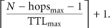${\text{TTL}}_{\max \hspace{0.17em}}$ nodes. Thus, the number of clusters can be given by

$\begin{array}{c}\lceil \frac{N-{\text{hops}}_{\max }-1}{{\text{TTL}}_{\max }}\rceil +1.\end{array}$

(6)

The number of clusters therefore is bounded by O(N). In practice, most clusters have more than TTL_max nodes, and therefore the number of cluster is lower than that in (6). However, as both the number of messages per cluster and the number of clusters are bounded by O(N), the worst-case message complexity is O( $N^2$ ).

Lemma 1 is a very loose bound, thus average complexity is derived next. Let $\lambda =N/A$ be the node density. Let us derive the message complexity of single-hop HHC scheme, that is, hops_max = 1 and TTL_max = 3, and similar arguments follows for SHC and multihop clusters [13]. In HHC, 1-hop and 2-hop neighbors further forward a cluster-formation broadcast. Altogether there will be $1+\{\lambda \pi r^2-1\}\hspace{0.17em}\hspace{0.17em}+\hspace{0.17em}\hspace{0.17em}\lambda \{\pi {(2r)}^2-\pi r^2\}=4\lambda \pi r^2$ broadcasts. Only nodes at a distance of 1-hop and 3-hops send ACKs back to the CH. Cost of forwarding these ACKs is $\lambda \pi r^2-1+3\lambda \{\pi {(3r)}^2-\pi {(2r)}^2\}=16\lambda \pi r^2-1$ . Up to six CCHs are selected as child CHs, and respective cluster formation requests travel up to 3-hops. Then the total overhead per cluster is $4\lambda \pi r^2+16\lambda \pi r^2-1+18=20\lambda \pi r^2+17$ . There are $A/k\pi r^2$ clusters in the network, where k is a constant that reflects the circularity of a cluster. Therefore, the total overhead is $20N/k\hspace{0.17em}\hspace{0.17em}+17A/k\pi r^2$ . Hence, the average message complexity is O(N).

2.3. Cluster Tree Self-Optimization Phase

Though the cluster tree formed with the HHC scheme is significantly better, it is suboptimal as the breadth and depth of the tree depend on several factors such as node distribution, which nodes are randomly selected as CCHs, and which of those selected CCHs are able to form clusters. A cluster-tree self-optimization phase is presented next that could further improve the breadth and depth of the tree.

Cluster tree self-optimization is performed by exchanging another set of messages among CHs. After the cluster formation phase, each CH (staring from the root node) sends at least one broadcast announcing its depth to neighboring CHs. A neighboring CH receiving this broadcast, checks whether the received depth is lower than its parent CH's depth. If so, the neighboring CH selects the broadcasting CH as its new parent CH and reorganizes its cluster tree membership. It then sends a new broadcast enabling its child and neighboring CHs to upgrade their depth. This approach increases the breadth of the cluster tree, while consequently reducing its depth.

Algorithm 2 formally describes this process. After the cluster formation phase, each of the CHs (except the root node) executes the Lstn_Optimize_Tree function to upgrade its depth in the cluster tree. The root node initiates the optimization phase by sending a broadcast (Bcast_CH_Presence) with its NID_CH, CID, and depth. When a broadcast is received, each CH compares its current depth (my_depth) with what was heard from its neighbor. If the new depth is lower, it sets the broadcasting CH as its new parent CH. After receiving the first broadcast, each CH generates a new broadcast with its own data (line 8). Even a CH that does not benefit from the new depth information, that is, current depth is lower, has to send its own broadcast once. This ensures that each CH receives at least one broadcast, and therefore gets the opportunity to upgrade its tree membership. If a CH hears a subsequent broadcast with even lower depth, it reorganizes the tree membership and regenerates a new broadcast with the updated depth.

Algorithm 2: Cluster tree self-optimization algorithm.

 Bcast_CH_Presence(NID _CH , CID, depth, TTL)

 Lstn_Optimize_Tree()

(1) Lstn_Bcast_CH_Presence ( ${NID}_{CH}$ , CID, depth)

(2) IF (my_depth > depth + 1)

(3)    my_CID ←CID

(4)    my_CH ← ${NID}_{CH}$

(5)    my_depth ←depth + 1

(6)    opt_msg_send ←FALSE

(7) IF (opt_msg_send = FALSE)

(8)    Bcast_CH_Presence ( ${NID}_{child}$ , my_CID, my_ depth, TTL)

(9)    opt_msg_send ←TRUE

The self-optimization algorithm is independent of the intercluster communication mechanism. Therefore optimization messages can be forwarded as either single (TTL = 1) or multiple (TTL = TTL_max) hop broadcasts. Single-hop broadcasts utilizing high-power therefore can directly reach nodes that were not reachable during the cluster formation phase (due to lack of intermediate nodes). This enables many CHs to improve their cluster tree membership. Consequently, breadth of the tree increases and depth reduces. During this phase, non-clustered nodes can join a nearby cluster if they hear a broadcast.

3. Routing

3.1. Cluster-Tree-Based Routing

Though many hierarchical routing schemes are designed to deliver data only towards the sink [1, 2, 9, 10], many WSN applications also require communication within the network [8, 14, 26]. If root node is either the sink or capable of forwarding messages to the sink, node-to-sink communication can be easily facilitated by forwarding data to upper levels in the cluster tree. However, an addressing scheme is required to facilitate node-to-node communication. Assume that the sender knows the destination address, through some other mechanism. In [27], we propose a mechanism to determine destination addresses in virtual sensor networks [14].

Our routing scheme makes use of the cluster tree formed with the HH C scheme (Figure 3) because of its desirable cluster and tree properties. Assume CH J wants to communicate with CH P. The message is first forwarded to C, as it is the parent CH of J. C only knows about its parent A and children J, K, and L. Therefore, C has to either drop the message or forward it to parent A. Even A does not know about P. This problem can be overcome by each CH keeping track of all its descendants. If C was aware that P is the child CH of L, it could have directly forwarded the message to L, which can forward it to P. As we go up the tree, more and more data about descendant CHs needs to be stored and the root node has to keep track of the entire network. This approach is not scalable in supporting communication among the nodes.

Figure 3

(a) A hypothetical sensor field covered with ideal HHC clusters; (b) corresponding cluster tree with hierarchical addresses. Scattered lines indicate cross-links among neighboring CHs.

A variable length hierarchical addressing scheme (Figure 3(b)) that reflects the parent-child relationship among CHs to overcome these issues is proposed next. A hierarchical address is assigned to a CH based on its branch number and parent CH's address. Branch numbers are relative to the parent CH and are determined based on the order that child CHs are selected from the set of CCHs. Branch numbers have a zero-based index. The root node (A) does not have a parent CH hence we assign its address as 0. B is the first child CH of A therefore gets address 00, second child C gets address 10, and G being the sixth child CH gets address 50. When B assigns addresses to its child CHs, it merges its address 00 with the child's branch number. Thus, the first child H gets address 000 while the second child I gets address 100. The branch related to H is discontinued as it does not have any child CHs. Q is the one and only child of I hence gets the address 0100. Address 210 is not assigned because the child CH that was given the address did not form its own cluster. Each CH is aware of the addresses of child CHs that were not able to form a cluster. If needed, such addresses can be reassigned to new child CHs that are added during the self-optimization phase. Then L, the fourth child, gets the address 310. The hierarchical addresses of each child CH is generated by the Select_Next_CID function of the GTC algorithm. Our addressing scheme satisfies all the necessary properties defined in [26].

To enable routing, each CH needs to keep track of only the addresses of its parent and child CHs. Root node keeps track of its immediate child CHs. Therefore, hierarchical addresses significantly reduce the number of routing entries at a CH. Given the hierarchical address of a destination, entire path to the destination can be determined. Next hop to forward a message can be determined using the pseudocode in Algorithm 3. A hierarchical address can be represented as an array of digits (Figure 3(b)) with the least significant digit (LSD) indicating the root node's branch number. The input variables current and destination indicate the hierarchical addresses of the CH that is trying to determine the next hop and the destination CH, respectively. Individual digits of the two addresses are compared starting from the LSD (line 4), until a mismatch is found. When the loop terminates, variable i indicates the number of matching digits. Digits that match indicate the address of the CH that two addresses converge. If i < Depth (current), the rendezvous is above the current CH hence the message should be forwarded to the parent CH. Otherwise, the rendezvous is below the current CH (line 9) and the message should go to one of the child CHs. Child CHs branch number can be determined from the ( $i+1$ )th digit in the destination address. For example, suppose CH L in Figure 3(b) wants to communicate with CH M. L's address is 310 while M's address is 020. Both addresses converge at the root node (A) as 0 is the only common digit between the two addresses (i.e., $i=1$ ). Because i < Depth (current), the message will be forwarded to the parent CH C. Similarly, when C compares its address with M's address, it realizes that the message needs to be forwarded to its parent CH A. As A is the rendezvous for the two addresses, the next hop should be one of A's child CHs. By looking at address 020, A can determine that message needs to be forwarded to child CH in the second branch, D. The message will be then forwarded from A to D. Two addresses 20 and 020 are compared again at D. Addresses are identical up to 20 hence next hop should be the child CH in branch zero. Thus, the message will be forwarded to the destination M.

Algorithm 3: Pseudo code to determine the next hop.

 Next_Hop(current, destination)

(1) IF (current = destination)

(2)   Return current

(3) min_depth ←Min(Depth (current), Depth (destination))

(4) FOR   $i=0$   TO min_depth

(5)   IF (current [i] ≠destination [i]

(6)     Break

(7) IF (i < Depth (current))

(8)   Return parent_CH

(9) ELSE IF (i = Depth (current))

(10)   Return  destination [ $i+1$ ]

3.2. Cross-Link-Based Routing

The root node is a single point of failure in hierarchical topologies. It spends energy much faster than the rest of the nodes, as it handles all the traffic going either to the base station or across different branches. If it is not energy constrained, its power limited child CHs will run out of energy faster than the remaining nodes as they share the traffic going through the root node. Multiple high-energy nodes can be placed closer to the root node to handle more traffic [28]. Yet such solutions are unable to utilize the energy available in rest of the network, which is critical in enabling communication within the network. We propose two routing approaches that make use of the energy available in rest of the CHs.

In a clustered network, neighboring clusters may belong to different branches of the cluster tree, for example, CHs H and J in Figure 3 belong to completely different branches of the tree. As they are in the same neighborhood, they can hear each other's messages and figure out each other's hierarchical addresses. Cross-links formed among such neighboring clusters can be used to forward messages across different branches of the cluster tree. For example, suppose H wants to communicate with K. A message travelling through the cluster tree will take the path $H\to B\to A\to C\to K$ , which is four-hops long. If H knows that its neighbor J is in the same branch as K, it can use J to relay the message. Then the new path $H\to J\to C\to K$ requires only three-hops. More importantly, it does not go through the root node. Ability to utilize such cross-links reduces the workload on the root node therefore increases the network lifetime.

It is not desirable to go through cross-links, just because they are available. The same hierarchical addresses can be used to determine whether it is shorter (or same) to go through the root node or across one of the cross-links. Given addresses of CHs H (000) and K (110), their rendezvous is the root node. Both H and K have two-hops to the root node hence the distance is four-hops. If H compares $J\text{'}\text{s}$ address (010) with K's address (110), their rendezvous is at a CH with address 10. Both J and K have a hop to the rendezvous and H also needs to forward the message to J, which requires another hop. Altogether, three-hops are required. Thus, shorter path through J is preferred. These changes can be easily incorporated into Algorithm 3 [13].

3.3. Circular-Path-Based Routing

More uniform and circular clusters of the same depth tend to be somewhat localized and lie on approximately concentric set of rings (see Figure 2). Therefore, as seen in Figure 4, cross-link based routing can be further extended by combining multiple cross-links that are at the same depth of the cluster tree to form circular-paths within the network. A path can be formed by sharing cluster addresses not only with the neighbors but also with neighbors of neighbors, if they lead to a better route. Such circular-paths enable many alternative routes without being tied to the cluster tree.

Figure 4

Cluster tree with a circular path constructed by connecting level 2 CHs that are in the same neighborhood.

Suppose a node in CH U (see Figure 4) wants to communicate with a node in CH K. A message going from U to K has to travel five-hops if it goes through the cluster tree. U is not in a circular-path; therefore, tree can be used to forward the message to its parent CH M. M is in the circular-path hence has the option of selecting either the circular-path (needs three-hops) or the cluster tree (needs four-hops). The route through circular-path is preferable as it is shorter and avoids the root node. The resulting route U→M→P→L→K is four hops long and utilizes both the tree and the circular-path.

To determine the path length, M has to know about K's address through neighboring CHs P and L, beforehand. It is not useful to share each CH's address with all the other CHs in a circular-path. For example, CHs H and P require four-hops to communicate with each other using either the tree or the circular-path. Circular-path is preferred as it reduces the burden on the root node. Therefore, it is useful for H and P to know about each other. For P's neighbor M, it takes four-hops to reach H through the tree and five-hops through the circular-path. Therefore, H's address is not useful to M and should not be propagated any further. Hierarchical addresses are useful in determining path lengths and making sure that only relevant addresses are shared among CHs along a circular-path. Though it is not possible to form a complete set of circles in a randomly deployed network, even partial circles are useful. Using a simplifying example it is possible to show that cluster tree with circular-paths has the largest lifetime.

Example 3.3.

Lower bound of network lifetime using the three routing schemes has the ordering: cluster tree with circular-paths > Cluster tree with cross-links > cluster tree.

Argument

Consider the lifetime of the network to be the time before the first node dies. Performance of node-to-node communication is evaluated as node-to-sink performance is same for all routing schemes. Assume nodes are homogeneous, and source and destination nodes are uniformly distributed across the network. It is complicated to derive the exact lifetime of the network considering depth/breadth of cluster tree and position of all source/destination nodes [13]. Therefore, a lower bound is derived by considering only the root node and level 1 CHs. Let CH₁ indicate a level 1 CH and λ be the packet arrival rate at a CH₁. In cluster-tree-based routing, a packet arriving at a CH₁ has to go to one of its descendants, to the root node, or to one of the remaining five level 1 clusters through the root node (Figure 3). Compared to the size of the network N, the root node has only a small number of cluster members. Therefore, it is reasonable to assume that each CH₁ is responsible for relaying packets to N/6 nodes. Hence, 1/6 of the packets will go to the descendants while remaining 5/6 will go across the root node. As there are six CH₁s, total load on the root node is 5λ. When cross-links are present, each CH₁ has two neighboring CH₁s (Figure 3). Then 1/6 of the packets will go to the descendants, 2/6 through neighboring CH₁s, and remaining 3/6 through the root node. Hence, the total load on the root node is 3λ. It can be shown that root node is still the bottleneck. Distance between any two CH₁s along the cluster tree is 2-hops (Figure 4). Therefore, when a circular-path is available each CH₁ keeps track of neighboring CH₁s that are within 2-hops. There are four such neighbors that could be used to reach 4N/6 nodes. However, CH₁s are now the bottlenecks because excessive use of the circular-path overloads them. A CH₁ has to forward λ packets originating from its descendants. In addition, its neighbors (two such neighbors) use it to reach 2/6 of the nodes while each of the remaining two-hop neighbors uses it to reach 1/6 of the nodes. Then the total load is λ + 4λ/6 + 2λ/6 = 2λ. Let P be the number of packets that can be relayed by a node. Therefore, lifetime of the network under each routing scheme is $P/5\lambda$ , $P/3\lambda$ , and $P/2\lambda$ which can be written as a set of ratios 1 : 1.667 : 2.5. Therefore, inequality holds.

Formation of cross-links and circular-paths at higher levels of the cluster tree will enable identification of better paths without coming all the way down to level 1. Therefore, the actual number of packets delivered by each routing scheme will exceed the lower bound.

4. Performance Analysis

4.1. Simulator

A discrete-event simulator is developed using C. 5000 nodes are randomly placed on a circular region with a radius of 500 m. The root node is placed in the middle of the sensor field. Single-hop clusters are formed using the breadth-first tree formation approach. Intercluster communication is single hop. Child CHs are selected randomly from a set of CCHs and for each simulation, the random function is initialized with a different seed. We compare our results with hexagonal packing that initiates from the root node. A circular sensor field is considered to make the comparison with hexagonal packing easier. Average circularity of clusters is defined as

$\text{Circularity}=\frac{1}{m}{\displaystyle \sum }_{i=1}^m\frac{\text{No}\hspace{0.17em}\hspace{0.17em}\text{of}\hspace{0.17em}\hspace{0.17em}\text{nodes}\hspace{0.17em}\hspace{0.17em}\text{in}\hspace{0.17em}\hspace{0.17em}\text{cluster}\hspace{0.17em}\hspace{0.17em}i}{\text{No}\hspace{0.17em}\hspace{0.17em}\text{of}\hspace{0.17em}\hspace{0.17em}\text{nodes}\hspace{0.17em}\hspace{0.17em}\text{in}\hspace{0.17em}\hspace{0.17em}\text{the}\hspace{0.17em}\hspace{0.17em}\text{range}\hspace{0.17em}\hspace{0.17em}\text{of}\hspace{0.17em}\hspace{0.17em}\text{C}{\text{H}}_i}\times 100,$

(7)

where m is the number of clusters in the network. Clusters at the border of the sensor field are often not able to find a sufficient number of nodes to achieve high circularity. However, these clusters have already attracted all the possible nodes. Our circularity metric assigns 100% to those clusters allowing us to discard the border effect. A hexagonal cluster in a uniformly distributed network has an average circularity of 82.7% [13]. Cluster tree formed with the HHC scheme is used while analyzing the performance of routing. Collisions among broadcasting nodes are considered. Signal propagation is based on the log-distance path-loss model [22] with a multipath fading factor of 2.2 [29]. Energy model is similar to that used in [1, 2] with each node having 2 J of energy. The results are based on 100 samples, which were sufficient to attain mean circularity, number of clusters, and number of messages within ±10% accuracy and 95% confidence level. Detailed simulation parameters can be found in [13] and the source code is available at [30].

4.2. Cluster and Cluster-Tree Characteristics

Figure 5 illustrates the physical shape of clusters formed by SHC and HHC schemes. Only the first SHC cluster has approximately a circular shape while the shapes of other clusters vary widely (Figure 5(a)). Child CHs are selected from nodes that are closer to the edge of the parent cluster, for example, CH of $c_3$ is within $c_1$ 's coverage area. Note that $c_i$ denotes the cluster labeled i. It is also possible that some of the child CHs reside inside the parent cluster, for example, CHs of $c_2$ and $c_4$ are inside $c_1$ . SHC may even form single node clusters, for example, $c_G$ and $c_F$ (see arrow in Figure 5(a)) initially had cluster members and they were later elected as CHs of $c_W$ and $c_{<}$ . SHC can push child CHs only up to the edge of the parent cluster, even with location information or RSSI, therefore clusters will overlap significantly. Alternatively, HHC clusters in Figure 5(b) are much larger, more circular, and have lower overlapping regions.

Figure 5

Physical shape of single-hop clusters: (a) SHC clusters; (b) HHC clusters. $Grid\hspace{0.17em}\hspace{0.17em}size=30\times 30$ , grid spacing = 5 units, nodes = 450, and transmission range = 30 units.

Circularity of single-hop clusters is summarized in Figure 6. HHC and RSSI heuristic-based HHC (R-HHC) clusters have much higher circularity than SHC. Ideal hexagonal clusters have the highest circularity. Ability to push CCHs further away from the parent CH reduces the overlap among most of the HHC clusters. However, as we push the CCHs further away, they can create coverage holes in the network (Figure 1(b)). Sometimes smaller clusters are formed to cover up such open regions, for example, $c_Z$ in Figure 5(b), while reducing the overall circularity. This is the reason that 5th percentiles for HHC and R-HHC overlap with 95th percentile of SHC. R-HHC clusters cover the sensor field more uniformly without creating such open regions, because the CCHs are selected from nodes that are just above 2hops_max from the parent CH. Uniform coverage requires some overlap among clusters; therefore, the circularity of R-HHC is relatively lower than that of HHC. Though uncertainties in signal strength affect R-HHC, it can still form clusters with better properties than HHC does [13].

Figure 6

Circularity of clusters. Error bars indicate the 5th and 95th percentile.

Due to the following factors, circularity reduces as the intracluster transmission power $P_T$ (i.e., transmission power of a node while forming clusters and communicating within a cluster) increases. When $P_T$ is higher, many nodes are capable of being selected as CCHs. The Wait_Lstn_Neighbors function prevents two nodes that are within each other's communication range (r) from becoming CCHs. However, clusters will overlap if the selected CCHs are within $2r$ from each other. High $P_T$ also increases collisions (even with random waiting), and thus some nodes may not hear a cluster-formation broadcast. Consequently, those isolated nodes may not join a cluster or later form smaller clusters. Coverage holes created by HHC scheme become larger as $P_T$ increases, consequently new clusters are formed to cover them up. These newly formed, small clusters overlap with the existing clusters consequently reducing the overall circularity.

Number of clusters/CHs produced by each scheme is shown in Figure 7. Number of clusters required to cover a given sensor field depends on both the circularity and geographical area covered by a cluster. Because of higher circularity, HHC produces a lower number of large clusters. As $P_T$ increases, the circularity of a cluster somewhat reduces while coverage area increases. However, increase in area is dominant (proportional to $r^2$ ). Therefore, number of clusters decreases with increasing $P_T$ . R-HHC produces a relatively higher number of clusters as it requires more clusters to cover the sensor field uniformly.

Figure 7

Number of clusters and cluster heads. Error bars indicate the 5th and 95th percentile.

We further evaluated the impact of node density on cluster characteristics. When the network is sparse, clusters are more circular. When it is dense, even a small coverage hole with one or two nodes needs to be covered by a new cluster. Consequently, circularity reduces with the increasing node density. Table 2 shows per node cluster and cluster-tree formation overhead. Uniform coverage property of R-HHC does not require the creation of new clusters to cover up coverage holes, and thus has the lowest overhead. Extra messages required by the post cluster-tree self-optimization phase (HHC-Opt) increase the overhead by approximately 1.5 messages per node, corresponding to around 25% increase. Per node overhead for different network sizes (N) are similar, which confirms that the average message complexity of GTC algorithm is O(N). We further build two other discrete-event simulators to compare HHC with FLOC [7] and the scheme given in [9]. While FLOC also shows a similar behavior for increasing $P_T$ and node density, HHC clusters are more circular and larger than FLOC clusters [13]. Multihop HHC clusters are more circular and larger than multihop clusters formed by scheme in [9], which probabilistically selects CHs. Cluster properties of HHC and ACE [6] are comparable. However, cluster formation overhead of HHC (Table 2) is much lower compared to that in ACE, which uses an iterative CH selection process.

Table 2

Number of control message per node. $P_T=-20$  dBm.

Scheme	$N=2500$	$N=5000$	$N=7500$
HHC	4.12	4.86	4.87
R-HHC	3.98	4.47	4.31
HHC-Opt	5.58	6.13	6.07

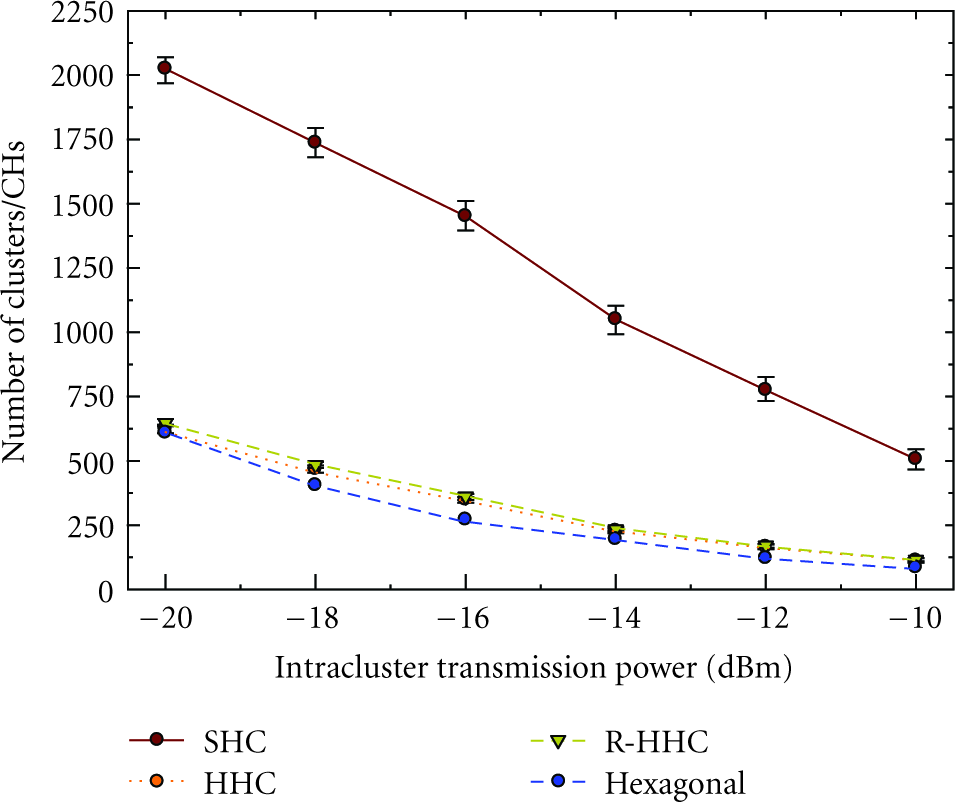
Figure 8 shows the distribution of CHs in the cluster tree. HHC and R-HHC schemes form much shorter trees than the SHC scheme. Due to high overlap among SHC clusters, some branches of the cluster tree are discontinued, resulting in a longer tree. Alternatively, HHC and R-HHC clusters are more uniformly distributed; therefore, tree has a higher branching factor and a lower depth. R-HHC selects a spatially distributed set of CCHs. Hence, most of the selected child CHs can form their clusters resulting in increased branching factor and reduced depth. Such a lower depth and higher breadth cluster tree is desirable in many WSN applications. The self-optimization phase reorganizes the cluster tree membership allowing a CH to connect to a new parent CH with a lower depth, while producing a shorter tree. Clusters become larger as $P_T$ increases. Consequently, fewer clusters are required to cover the sensor field and the depth of the tree reduces.

Figure 8

Distribution of CHs at different levels of the cluster tree: (a) $P_T=-20$  dBm; (b) $P_T=-10$  dBm.

Physical shape of the cluster tree formed by one of the data samples is shown in Figure 9(a). Figure 9(b) shows the same tree after the cluster-tree self-optimization phase. The optimized tree is more structured and shorter than the original one. In addition to the maximum depth (see Table 3), the number of intersecting links and CHs having higher depth than their distant neighbors can be used to determine the orderliness and regularity of a cluster tree. In Figure 9(a), links AB and AC intersect link DE. Such intersections are not desirable as they could lead to collisions during intercluster communication. Original tree has 34 intersections and it is reduced to 15 in the optimized tree. Furthermore, node E is physically more closer to the root node than node A yet its depth is 3-hops higher than that of A. Such cases should be avoided as they unnecessarily increase the path length, and therefore increase the energy consumption and latency. Original tree has 24 such CHs and all of them are removed in the optimized tree. Thus, optimized tree is more structured. Note that after the optimization phase all the disconnected nodes in Figure 9(a) are connected to a cluster.

Table 3

Comparison of theoretical and empirical depth of the cluster tree.

$P_T$	Scheme	Depth-theoretical	Depth-empirical
−20 dBm	HHC	15	15
	R-HHC		14
	HHC-Opt		14
−10 dBm	HHC	5	8
	R-HHC		7
	HHC-Opt		4

Figure 9

Physical shape of the cluster tree formed with HHC scheme: (a) before optimization; (b) after optimization. $N=5000$ , $P_T=-12$  dBm, squares—CHs, and circles—nodes without a cluster.

Such a structured topology reduces path length and latency, and can be used to build an addressing scheme that reflects the geographical location of CHs, for example, using an approach similar to that in [31]. Simulation results and the depth predicted by (3) are compared in Table 3. For lower $P_T$ , empirical depth is within the bound predicted by the model. Cluster properties are less optimal for higher $P_T$ , and therefore form a relatively longer tree. However, as we can see from Figures 8 and 9, and Table 3, the self-optimization phase significantly improves such cluster trees. This demonstrates that cluster properties are comparable with hexagonal packing for lower $P_T$ and sparse networks, and that the model based on hexagonal packing is valid for such cases.

4.3. Performance of Routing

After the cluster formation phase, each CH sends a broadcast with its hierarchical address allowing its neighbors to form cross-links. Circular-path based routing requires the formation of set of rings within the network by connecting CHs at the same depth. In practice, it may not be possible to build a closed ring because CHs with same depth may not lie on a set of concentric rings and could further depend on node positions and physical shape of clusters. Therefore, we relax the same depth constraint by allowing a CH to share addresses with neighboring CHs, if neighbors' depth is one level higher than its own depth. Messages are sent between randomly selected source and destination node pairs. For comparison, we take the number of messages delivered until the first node dies.

Figure 10 shows the number of messages delivered by each routing scheme. Use of cross-links reduces the workload on the root node, and therefore increases the message capacity by 2.1–2.4 times than routing with only the cluster tree. Circular-paths distribute the workload across many CHs, therefore they deliver 2.7–3.2 times more messages. Relaxed circular-path construction (Circular + 1) increases the capacity by 5.2–6.4 times. The cluster-tree self-optimization phase forms a more structured topology allowing even better construction of circular-paths. Therefore, circular-path routing on top of the optimized tree (Tree (Opt) + Circular) is able to deliver 3.6–5.5 times more messages while relaxed circular-path construction delivers 6.0–8.1 times more messages. Tree-based and cross-link-based routing schemes are unable to benefit from the self-optimization phase because the root node is the bottleneck (see the example in Section 3.3). Nevertheless, all routing schemes benefit from shorter routes along the optimized tree, and therefore become more suitable for latency bound sensor applications. All the routing schemes deliver lower number of messages with increasing $P_T$ as high-power transmissions significantly drain energy at a CH.

Figure 10

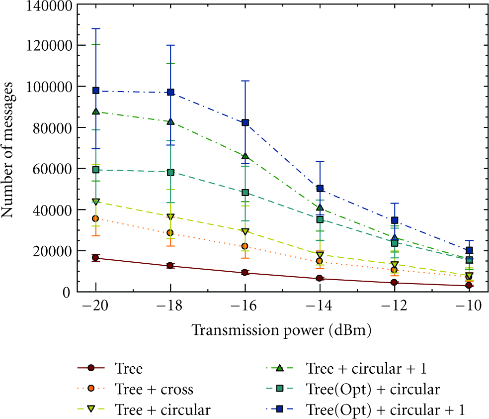
Number of messages delivered by each routing scheme. Error bars indicate the 5th and 95th percentile.

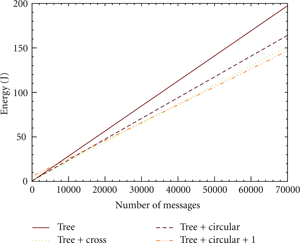
Average residual energy of CHs at the end of the network lifetime is shown in Figure 11. The root node depleted its energy in both cluster-tree-based and cross-link-based routing. For circular-paths, however, the bottleneck is among CHs between depths 1–4; thus, the bottleneck has shifted to the middle of the tree. Relaxed circular-path construction scheme is able to distribute the workload even more and utilizes energy available in CHs between depths 1–8, thereby delivering a significantly higher number of messages. This behavior of the routing schemes further confirms the analysis of example in Section 3.3. Figure 12 shows the energy consumption of the network assuming nodes have sufficient power to stay active for a long time. Cluster formation and address discovery overhead are constant. Therefore, all the routing schemes linearly increase the number of delivered messages as the energy per node increases, a behavior confirmed by simulation results as well. Though relaxed circular-path construction has the highest initial overhead (due to address sharing with many nodes), it performs best by being able to send a large number of messages over a long period. It reduces the energy per message by identifying shorter routes and thus significantly extends the network lifetime by distributing the workload across many CHs. Circular-path based routing's ability to distribute the workload while alleviating hotspots is desirable in WSNs that are capable of harnessing energy, where it allows sufficient time for nodes to regain energy thus extending the network lifetime.

Figure 11

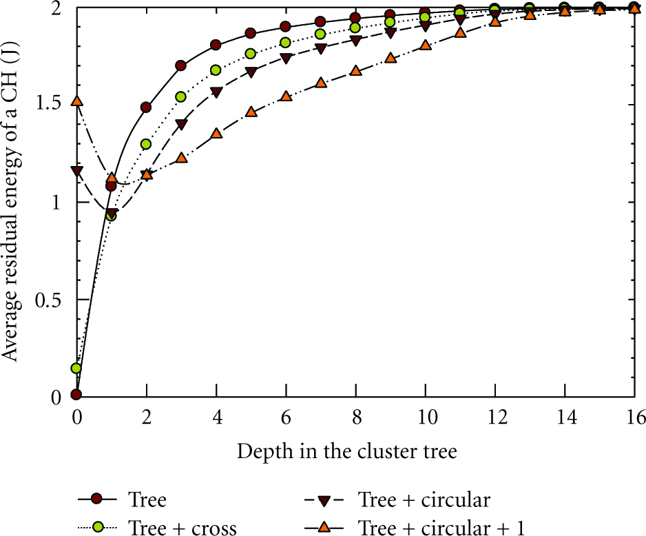
Average residual energy of CHs at different depths of the cluster tree at the end of the network lifetime. $P_T=-20$  dBm.

Figure 12

Energy consumption of the network with time. $P_T=-20$  dBm.

5. Conclusions

A top-down cluster and cluster-tree formation algorithm that is independent of network topology, and does not require a priori neighborhood information, location awareness, or time synchronization is presented. GTC is configurable where parameters such as the number of nodes in a cluster and breadth/depth of the cluster tree can be controlled. For example, the HHC scheme of the GTC algorithm forms more uniform clusters and a cluster tree with a lower depth. RSSI-based heuristic forms even more uniform and circular clusters and a shorter tree, but relies on RSSI for distance estimation. Cluster and tree properties are comparable to hexagonal packing for low intracluster transmission power levels and sparse networks. The post cluster-tree self-optimization phase forms an ordered cluster tree and reduces its depth. Therefore, it is desirable in latency-bound applications. Hierarchical addresses based cluster tree routing facilitates communication within the network as well as with the base station. Cross-link-based and circular-path-based routing schemes increase the network lifetime by two and three times, respectively. Relaxed heuristic based circular-path construction improves the lifetime by five-times while it gains a six to eightfold improvement when self-optimization is enforced. It performs best over a long period, thus it is desirable for networks that exist over a very long period and networks with nodes that harness energy. In [27], we proposed a cluster-tree-based implementation of virtual sensor networks [14], and demonstrated the efficacy of our scheme by simulating a subsurface chemical plume monitoring system [13].