Sage Journals: Discover world-class research

Abstract

The constrained power source given by batteries has become one of the biggest hurdles for wireless sensor networks to prevail. A common technique to reduce energy consumption is to put sensors to sleep between duties. It leads to a tradeoff between making a fewer number of observations for saving energy while obtaining sufficient and more valuable sensing information. In this paper, we employ two model-based approaches for tackling the sensor scheduling problem. The first approach is to apply our corrected VoIDP algorithm on a chain graphical model for selecting a subset of observations that minimizes the overall uncertainty. The second approach is to find a selection of observations based on Gaussian process model that maximizes the entropy and the mutual information criteria, respectively. We compare their performances in terms of predictive accuracies for the unobserved time points based on their selections of observations. Experimental results show that the Gaussian process model-based method achieves higher predictive accuracy if sensor data are accurate. However, when observations have errors, its performance degrades quickly. In contrast, the graphical model-based approach is more robust and error tolerant.

1. Introduction

The technology of wireless sensor networks has been popular for more than a decade in both academia and industry. Through the observations obtained by tiny embedded wireless sensors, we can have a better understanding of the natural environment, human activities, and their interactions. Researchers have been trying to turn the current relatively small-scale wireless sensor networks to a future generation of large-scale, energy-sustainable, and extensively long-standing deployments. One of the biggest hurdles is the constrained power source. Today's wireless sensors are mostly battery powered. It is not a viable way for human intervention to replace the batteries for thousands of wireless sensor nodes. The high maintenance overhead prevents the wireless sensing technology from prevailing in real-world large-scale applications.

A common technique for extending the lifetime of a wireless sensor network is to reduce its duty cycles, that is, a sensor wakes up for a small amount of time in a fixed period of interval to sense and go to sleep the rest of the time. Besides reducing sensing times for saving energy, it would be desirable to have the informative values obtained from the sensing data as high as possible. The observations should be worth of their energy costs. This is even more important for the next generation of scalable wireless networked sensors.

Tomorrow's sensors will be much smaller and energy sustainable. They can harvest energy from the environment [1]. The ambient power sources in their surrounding such as heats, mechanical movements, electromagnetic induction, and electrochemical reactions make sensing more sustainable and hassle free. However, energy harvesting on wireless sensors also brings a lot of challenges. First of all, the ambient power supply is often intermittent, and the smaller the sensor nodes are, the less power they can store. Moreover, the harvested energy usually needs to be accumulated to reach a certain level before being capable of performing some operations like taking a sensor reading or transmitting a packet. In such situations, the energy harvested sedulously should never be taken for granted. Instead, every sensing observation paid by the harvested energy should be as rewarding as possible.

Making optimal scheduling of observations with a limited power budget to maximize their information gains has become an important problem in real-world applications. It is a trade-off between obtaining more and useful information versus making less observations. The optimization of selecting observations can be considered as a subset selection problem. For example, in a task of monitoring indoor temperature, if a wireless sensor is deployed to observe for only once per hour, and we want to turn on the sensor k times for a day, then it becomes such a subset selection problem that k out of the total 24 time points are chosen so that the k observations will be the best selection among the other options for having the most accurate predictions of temperature readings at the unobserved time points.

In the context of statistics, the problem of subset selection or variable selection determines a subset of variables and eliminates the rest from usually a linear regression model, in order to increase predictive accuracy or to get the “big picture” with the strongest effects of predictors [2, 3]. But the selection of variables are usually for predicting only a single variable of interest. However, in the sensor scheduling case, the subset selection needs to predict the temperature distribution that covers all the unobserved time points.

Probabilistic inference in graphical models [4] provides an effective tool to deal with the quantification of uncertainty existed in the subset selection problem. The optimal subset of observations is the one that minimizes the uncertainty of the posterior conditional probability distribution of the unobserved variables. Hidden Markov models (HMMs), the chain graphical models, are often used for modelling time series data. The posterior conditional probability of unobserved variables given observations can be efficiently computed on an HMM. The VoIDP algorithm [5] was claimed to be the first optimal algorithm for efficiently making the subset selection on the chain graphical models. The name “VoIDP” was after its usage of dynamic programming approach to optimize the information value. We corrected the original VoIDP algorithm by fixing a mistake in it [6]. In this paper, we apply the corrected version of VoIDP algorithm on an HMM to solve the subset selection problem for sensor scheduling.

Gaussian process (GP) is a generalization of linear regression based on multivariate normal distributions [7]. It is often applied to spatial monitoring problems [8, 9]. Greedy methods based on heuristics, such as entropy and mutual information, can efficiently make a selection of time points. The mutual information [10] criterion, which measures entropy reduction, was shown to have better solutions than the entropy criterion in a couple of sensor placement problems [8]. In this paper, we use the GP-based approach with both the entropy and mutual information heuristics to solve the sensor scheduling problem.

In summary, the objective of the sensor scheduling problem is to select a subset of time points to turn on a sensor and keep it off at the other time to minimize prediction errors at unobserved time points. Our contribution is employing the GP model-based selection approach and our corrected version of VoIDP algorithm based on graphical models to solve the scheduling problem and comparing their performances. The GP-based approach is more data driven than the graphical model-based approach. But the latter, such as an HMM, can capture the underlying structures of the latent variables that determine the observational values in time series. Through comparison experiments, we find out that the GP-based selection approach achieves lower prediction error than the HMM-based approach given with accurate observations. However, the HMM-based selection approach performs more stably and robustly than the GP-based approach with erroneous observations.

We will briefly describe the graphical model-based, particularly HMM-based, selection approach in Section 2, and the GP-based selection approach in Section 3. The experimental results will be presented and discussed in Section 4. Following that are the conclusions.

2. Probabilistic Graphical-Model-Based Observation Selection

A sensor's time series of observations can be modeled using a probabilistic graphical model, such as an HMM. Each observation variable at a timepoint has a distribution over some hidden states such as different time periods or some events. Any observations made on the chain graphical model will contribute to the predictions of values for other unobserved variables. But the degree of the contributions depends on the selection of observations.

The quality of a selection of observations is measured based on how the observation subset changes the shape of the probability distribution of an unobserved variable. The probability distribution of any unobserved variable conditioned on a subset of observed variables can be efficiently computed using a trained HMM. A utility reward can thus be defined by the entropy on the posterior conditional probability distribution. When a subset of observation variables is selected, an expected total reward across the entire time chain is computed. Hence, the sensor scheduling problem can be formulated as a subset selection problem on a chain graphical model as follows.

Given random variables $𝒳_{𝒱} = (𝒳_{1}, \dots, 𝒳_{n})$ , a subset of the variables, $𝒳_{𝒜} = (𝒳_{i_{1}}, \dots, 𝒳_{i_{k}})$ is observed as $x_{𝒜}$ . $P (𝒳_{𝒱} | 𝒳_{𝒜} = x_{𝒜})$ is the conditional observation distribution over all variables given the observation $x_{𝒜}$ . A total reward $R (P (𝒳_{𝒱} | 𝒳_{𝒜} = x_{𝒜}))$ is also given. The subset selection problem is

A^{*} = {\arg \max}_{A} \sum_{x_{A}} P (X_{A} = x_{A}) R (P (X_{V} | X_{A} = x_{A})),

(1)

where the expected total reward is used because the future observations of

𝒳_{𝒜}

are unknown. The selections are made based on the model before knowing any observational values. Because of conditional independency on chain graphical models, the expected total reward to maximize in (1) is also the summation of all the expected local rewards, where an expected local reward

R_{j} (𝒳_{j} | 𝒳_{𝒜})

equals to

\sum_{x_{𝒜}} P (𝒳_{𝒜} = x_{𝒜}) R_{j} (𝒳_{j} | x_{𝒜})

. A local reward

R_{j} (𝒳_{j} | x_{𝒜})

depends on

P (𝒳_{j} | 𝒳_{𝒜} = x_{𝒜})

, which is the marginal distribution of variable

𝒳_{j}

conditioned on observations

𝒳_{𝒜} = x_{𝒜}

. We can define the reward by using conditional entropy, that is,

R_{j} (𝒳_{j} | x_{𝒜}) = - H (𝒳_{j} | x_{𝒜}) = \int P (x_{j}, x_{𝒜}) \log_{2} P (x_{j} | x_{𝒜}) d x_{j}

The conditional independence property of chain graphical models simplifies the evaluation of $P (𝒳_{j} | 𝒳_{𝒜})$ . If only the observations made before a time point are used, then the evaluation of $P (𝒳_{j} | 𝒳_{𝒜})$ only depends on $P (𝒳_{j} | 𝒳_{i})$ , where $𝒳_{i}$ is the closest observation made before j. Moreover, the conditional independence property also decomposes the expected total reward for the entire chain into the local rewards for subchains that are separated by the observations. This important property inspired an efficient approximate algorithm based on the divide-and-conquer strategy [5].

The subset selection problem in (1) is a combinatorial optimization problem like the Knapsack problem, although its utility function is more computationally complicated. It is an NP-hard problem. The Knapsack problem admits a pseudopolynomial time algorithm, and all known such algorithms for NP-hard problems are based on dynamic programming [11].

The authors in [5, 12] developed an algorithm called VoIDP to solve the subset selection problem, and it was claimed to be the first optimal algorithm for selecting the optimal observations on chain graphical models. It implements a dynamic programming approach that exploits the chain structured models to efficiently evaluate the expected total reward. The time complexity of the algorithm was proved to be $(1 / 6 n^{3} + 𝒪 (n^{2})) B$ given budget B in terms of the number of evaluations of the rewards, where $n = | 𝒱 |$ . Although it works efficiently and optimally with a chain graphical model, it is still much harder to be applied on more general forms of graphical models. It was proved that the problem of selecting a subset of observations for even discrete poly-tree is computational intractable.

We found out a mistake in the originally published VoIDP algorithm that fails to give correct solution. We corrected the mistake and presented an improved version of the algorithm in [6]. In the experiments, we will use the corrected VoIDP algorithm that will be briefly presented in what follows. Once the optimal observations are selected, the predictive value will be calculated by taking the expected mean of a posterior conditional observation distribution.

Algorithm 1 shows the corrected version of VoIDP. The first part of the algorithm dynamically computes a three-dimension ( $a, b, and k$ ) table, where a and b are the two ends of a chain, and k is the budget. Each cell in the table is a tuple of two elements: $L_{a : b} (k)$ and $Φ_{a : b} (k)$ . $L_{a : b} (k)$ represents the optimal expected total reward of the subchain $a : b$ with the budget k. $s e l (j)$ is the expected total reward of the subchain $a : b$ obtained by observing at time point j, and $s e l (0)$ is the reward when no observation is made. $Φ_{a : b} (k)$ stores the j that maximizes the value of $s e l (j)$ . $L_{a : b} (0)$ is the base case, and the recursion for $L_{a : b} (k)$ is either $L_{a : b} (0)$ or $ma x_{a < j < b, β_{j} \leq k} {s e l (j)}$ . It means that we can choose not to spend any more of the budget to reach the base case, or select the optimal observation at j with the cost $β_{j}$ . $C_{j}$ denotes penalty on the reward by selecting at j. In our experiments, we let $C_{j}$ be zero and $β_{j}$ be one.

Algorithm 1: Corrected VoIDP algorithm for optimizing observation selection on chain graphical models.

Input: Budget B, rewards $R_{j}$ , costs $β_{j}$ and penalties $C_{j}$

$(j \in 𝒱, | 𝒱 | = n)$

Output: Optimal selection of observations at 𝒜

begin

for $0 \leq a < b \leq n + 1$ do compute $L_{a : b} (0)$

for $k = 1$ to B do

for $0 \leq a < b \leq n + 1$ do

$s e l (0) \leftarrow L_{a : b} (0)$

for $j = a + 1$ to $b - 1$ do

$s e l (j) \leftarrow$

$R_{j} (𝒳_{j} | 𝒳_{j}) - C_{j} + L_{a : j} (0) + L_{j : b} (k - β_{j})$

$L_{a : b} (k) \leftarrow \max_{j \in {0, a + 1, \dots, b - 1}} s e l (j)$

$Φ_{a : b} (k) \leftarrow {\arg \max}_{j \in {0, a + 1, \dots, b - 1}} s e l (j)$

$a \leftarrow 0; b \leftarrow n + 1$

$k \leftarrow B$

$𝒜 \leftarrow \emptyset$

repeat

$y \leftarrow Φ_{a : b} (k)$

if $y > 0$ then

$𝒜 \leftarrow 𝒜 \cup {y}$

$a \leftarrow y$

$k \leftarrow k - β_{y}$

else

break

until $k \leq 0$

The second part of Algorithm 1 computes the optimal selections by tracking through the values of $Φ_{a : b} (k)$ . Initially a and b are set to represent the entire chain. It starts with the full budget B and the empty selection set 𝒜. In the following loop, it finds the optimal selection y from $Φ_{a : b} (k)$ , and adds it into the selection set 𝒜. Whenever a selection is made, it spent a budget of $β_{y}$ and cuts the chain into two parts, a : y and y : b. The searching of optimal observation will be continued on the second subchain y : b. This process will stop when the budget is used up. The bold-faced $a \leftarrow y$ is important because it makes the tracking to fall into the correct domain in the whole table, but it was not in the original VoIDP algorithm.

3. Gaussian Process-Based Observation Selection

A Gaussian process (GP), by definition [7], is a collection of random variables, and any finite number of variables in the collection also has a joint Gaussian distribution. For scheduling a sensor, we assume that the joint probability of its observations at all the time points is a multivariate Gaussian distribution:

\begin{matrix} P (X_{V} = x_{V}) = \frac{1}{{(2 π)}^{n / 2} {| Σ_{V V} |}^{1 / 2}} e^{- 1 / 2 {(x_{V} - μ_{V})}^{T} Σ_{V V}^{- 1} (x_{V} - μ_{V})} \end{matrix},

(2)

where 𝒱 denotes the whole set of the variable indices with

| 𝒱 | = n

μ_{𝒱}

is the mean vector and

Σ_{𝒱 𝒱}

is the covariance matrix. A subset 𝒜 from 𝒱 also satisfies that

𝒳_{𝒜} ~ 𝒩 (μ_{𝒜}, Σ_{𝒜 𝒜})

, where

μ_{𝒜}

is a subvector of

μ_{𝒱}

and

Σ_{𝒜 𝒜}

is the relevant submatrix of

Σ_{𝒱 𝒱}

. This consistency property is also known as the marginalization property.

The nice property also holds in $P (𝒳_{i} | 𝒳_{𝒜} = x_{𝒜})$ , the probability distribution of $𝒳_{i}$ conditioned on the observational values $x_{𝒜}$ of a selected variable set $𝒳_{𝒜}$ . This posterior conditional probability is also a Gaussian distribution with conditional mean $μ_{i | 𝒜}$ and variance $σ_{i | 𝒜}^{2}$ given by

\begin{gathered} μ_{i | A} = μ_{i} + Σ_{i A} Σ_{A A}^{- 1} (x_{A} - μ_{A}), \end{gathered}

(3)

\begin{gathered} σ_{i | A}^{2} = Σ_{i i} - Σ_{i A} Σ_{A A}^{- 1} Σ_{A i}, \end{gathered}

(4)

where

μ_{𝒜}

is the mean vector of variable set

𝒳_{𝒜}

Σ_{i 𝒜}

, and

Σ_{𝒜 i}

are the corresponding submatrices of

Σ_{𝒱 𝒱}

. For instance, the

Σ_{i 𝒜}

is calculated by taking the ith row and the 𝒜 columns of

Σ_{𝒱 𝒱}

μ_{i}

and

Σ_{i i}

can be considered as the prior mean and the prior variance of the observations at i.

3.1. The Entropy Heuristic

The conditional probability $P (𝒳_{i} | 𝒳_{𝒜})$ carries very important information for evaluating the quality of the selection set 𝒜, which can be measured by the conditional entropy:

\begin{matrix} H (X_{i} | X_{A}) & = - \int \int P (x_{i}, x_{A}) \log P (x_{i} | x_{A}) d x_{i} d x_{A} \\ = \frac{1}{2} \log σ_{i | A}^{2} + \frac{1}{2} (\log π + \log 2 + 1), \end{matrix}

(5)

where

P (𝒳_{i} | 𝒳_{𝒜})

is assumed as a Gaussian probability distribution. Note that the entropy is a monotonic function of its variance

σ_{i | 𝒜}^{2}

, which can be evaluated ahead of making any observations (4).

The sensor scheduling problem becomes to select a subset of time points at 𝒜 (out of the variable index set 𝒱) to turn on the sensor and to keep it off at all the other time (as of indices in $𝒱 ∖ 𝒜$ ). The subset selection can be optimized by minimizing the entropy $H (𝒳_{𝒱 ∖ 𝒜} | 𝒳_{𝒜})$ . This is also equivalent to finding a subset 𝒜 that maximizes $H (𝒳_{𝒜})$ , as the chain rule for conditional entropy holds that $H (𝒳_{𝒱 ∖ 𝒜} | 𝒳_{𝒜}) = H (𝒳_{𝒱}) - H (𝒳_{𝒜})$ . The optimization problem turns out to be an NP-hard problem. To solve it, a greedy heuristic is to iteratively find the next selection $y_{i + 1}^{*} \in 𝒱 ∖ 𝒜_{i}$ that has the highest conditional entropy given the current selection set $𝒜_{i}$ :

\begin{matrix} y_{i + 1}^{*} = {\arg \max}_{y_{i + 1}} H (X_{y_{i + 1}} | X_{A_{i}}) \end{matrix} .

(6)

Algorithm 2 shows the greedy algorithm based on the entropy heuristic. k is the size of the selection and the $σ_{y | 𝒜}^{2}$ can be computed using (4). Because the log function is monotonic, $σ_{y | 𝒜}^{2}$ is proportional to $H (𝒳_{y} | 𝒳_{𝒜})$ . That means finding a selection at y that maximizes $H (𝒳_{y} | 𝒳_{𝒜})$ is equivalent to finding such a y that maximizes $σ_{y | 𝒜}^{2}$ .

Algorithm 2: Greedy algorithm for maximizing entropy $H (𝒜)$ .

Input: covariance matrix $Σ_{𝒱 𝒱}$ , selection size k

Output: selection set $𝒜 (𝒜 \subseteq 𝒱, and | 𝒜 | = k)$

begin

$𝒜 \leftarrow \emptyset$

for $i = 1$ to k do

foreach $y \in 𝒱 ∖ 𝒜$ do $δ_{y} \leftarrow σ_{y | 𝒜}^{2}$

$y^{*} \leftarrow {\arg \max}_{y \in 𝒱 ∖ 𝒜} δ_{y}$

$𝒜 \leftarrow 𝒜 \cup {y^{*}}$

The computation of $σ_{y | 𝒜}^{2}$ is expensive. Let $| 𝒱 | = n$ , there are n times of these computations when $i = 1$ , and $(n - k + 1)$ times when $i = k$ . Hence, Algorithm 2 has totally $(2 n - k + 1) k / 2$ times of evaluations of $σ_{y | 𝒜}^{2}$ .

3.2. The Mutual Information Heuristic

Another criterion for optimizing the subset selection is the mutual information, which was originally proposed by Caselton and Zidek in [10]. The mutual information of a subset 𝒜 denoted as $MI (𝒜)$ is defined as follows, and it is actually the entropy reduction:

\begin{matrix} M I (A) & = I (X_{V ∖ A}; X_{A}) \\ = H (X_{V ∖ A}) - H (X_{V ∖ A} | X_{A}) \\ = H (X_{A}) - H (X_{A} | X_{V ∖ A}) . \end{matrix}

(7)

The authors in [8] demonstrated the advantage of the mutual information criterion over the entropy criterion in sensor placement for a couple of spatial monitoring applications. They found out that the mutual information criterion led to a more intuitive sensor placement than the entropy criterion did. The mutual information criterion placed sensors in the central areas of a sensing space whereas the entropy placed sensors mostly at the boundaries.

In contrast to the entropy-based selection maximizing only the uncertainty of the selection set 𝒜, the mutual information criterion maximizes the reduction of the entropy over the rest of the variable space $𝒱 ∖ 𝒜$ before and after observing at 𝒜. That is, to schedule a sensor, we will find a subset of time points at $𝒜^{*}$ such that

\begin{matrix} A^{*} = {\arg \max}_{A \subset V} M I (A) \end{matrix} .

(8)

Optimization of the mutual information is also an NP-complete problem. A greedy algorithm was developed in [8] that selects the next variable y maximizing the mutual information gain:

\begin{matrix} Δ_{y} = M I (A \cup y) - M I (A) . \end{matrix}

(9)

The greedy heuristic chooses the next selection that provides the maximal increase in the values of mutual information.

In the context of Gaussian process and based on the entropy equation in (5), (9) can be further deduced as:

\begin{matrix} Δ_{y} & = M I (A \cup y) - M I (A) \\ = H (y | A) - H (y | \bar{A}) \\ = \frac{1}{2} \log_{2} (\frac{σ_{y | A}^{2}}{σ_{y | \bar{A}}^{2}}), \end{matrix}

(10)

where

\bar{𝒜}

means all the variable indices in 𝒱 excluding 𝒜 and y, which can also be denoted as

𝒱 ∖ (𝒜 \cup y)

An interesting note about the mutual information gain $Δ_{y}$ is that it is monotonically decreasing as the selection set 𝒜 gets larger. It inspired the enhanced greedy algorithm with lazy evaluation [8].

The greedy algorithm with lazy evaluation for maximizing the mutual information is presented in Algorithm 3. We rewrite it as in the context of the Gaussian process model.

Algorithm 3: Greedy algorithm for maximizing mutual information gain $M I (𝒜 \cup y) - M I (𝒜)$ using lazy evaluation.

Input: covariance matrix $Σ_{𝒱 𝒱}$ , selection size k

Output: selection set $𝒜 (𝒜 \subseteq 𝒱)$ , mutual information

gains $Δ$

begin

$𝒜 \leftarrow \emptyset$

foreach $y \in 𝒱$ do $Δ_{y} \leftarrow + \infty$ ; $Φ_{y} \leftarrow 0$

for $i = 1$ to k do

repeat

$y^{*} \leftarrow {\arg \max}_{y \in 𝒱 ∖ 𝒜} Δ_{y}$

if $Φ_{y^{*}} = = i$ then

break

else

$\bar{𝒜} \leftarrow 𝒱 - (𝒜 \cup y^{*})$

$Δ_{y^{*}} \leftarrow 1 / 2 \log_{2} (σ_{y^{*} | 𝒜}^{2} / σ_{y^{*} | \bar{𝒜}}^{2})$

$Φ_{y^{*}} \leftarrow i$

until 0

$𝒜 \leftarrow 𝒜 \cup {y^{*}}$

$Φ_{y^{*}}$ records in which iteration $Δ_{y^{*}}$ is updated. The lazy evaluation saves a lot of computation of $Δ_{y}$ based on the insight that the sequence of the mutual information gains on a fixed y decreases as set 𝒜 gets bigger. It will select the $y^{*}$ if the maximal $Δ_{y^{*}}$ is updated in the current iteration, otherwise it will update $Δ_{y^{*}}$ and $Φ_{y^{*}}$ and repeat the selection process.

When $| 𝒱 | = n$ , Algorithm 3 has $2 (n + k - 1)$ times of evaluations of either $σ_{y^{*} | 𝒜}^{2}$ or $σ_{y^{*} | \bar{𝒜}}^{2}$ in the best case. This is more efficient and scalable than Algorithm 2 when n becomes very large.

Algorithm 3 is not only efficient, but also provides its solution with a theoretic bound to the optimal solution. Although the mutual information function in (7) is not always increasing, the authors in [8] proved that it is still a partially monotonic submodular function. According to [13], a greedy algorithm, such as the Algorithm 3, which optimizes a monotonic submodular function guarantees a theoretical performance lower bound of $(1 - 1 / e) OPT$ , where $OPT$ is the optimal solution value.

After a subset of observations at 𝒜 is selected, the conditional probability distribution of an unobserved variable i given the observations of $𝒳_{𝒜}$ can be computed as $P (𝒳_{i} | 𝒳_{𝒜})$ . We will use its mean computed by (3) as the predictive value of the observation variable $𝒳_{i}$ .

4. Comparison Experiments

In this section, we will compare the probabilistic graphical model-based approach and the Gaussian process model-based approach in solving the subset selection problem for scheduling a sensor. Specifically, we want to select a subset of time points in size k out of totally 24 time points for turning on a sensor to sense and keeping it off at the other time. For convenience, in the following experiments, we will refer to the probabilistic graphical model-based approach simply as the HMM-based method, and the Gaussian Process-based approach simply as the GP-based method. The performance is measured using predictive accuracy for the unobserved time points in terms of the root mean squares (RMS) error. The methods are compared for accurate observations, as well as erroneous observations.

4.1. Experimental Setup

A hidden Markov model and a multivariate Gaussian model were trained using the temperature time series data collected in the Intel Berkeley Research Laboratory [14]. All the data were preprocessed for missing samples and discretized into 10 bins of 2 degrees Kelvin. The full dataset consists of temperature samples combined from three neighbored sensors for 19 days. When training the chain graphical model, we set four latent states representing the different time periods 12 am–7am, 7 am–12 pm, 12 pm–7 pm, and 7 pm–12 am. The whole dataset was also randomly split into the test set and the training set with the ratio 1 : 9. A small error-injected test dataset was also generated. The errors were taken randomly from a normal distribution with mean zero and variance 0.25.

We use these notations in the figures: “hmm_voidp” represents the HMM-based selection approach by our improved VoIDP algorithm; “gp_entropy” represents the GP-based selection approach by employing the entropy heuristic, and “gp_mutual” for the GP-based mutual information heuristic.

4.2. Results and Discussion

Figures 1(a) and 1(b) show the results on the full dataset. Generally speaking, the more observations are selected the less RMS prediction errors are achieved for both the HMM based and the GP based approaches. In Figure 1(b), the mutual information heuristic holds the competition with the entropy heuristic until about 10 observations are selected. We have mentioned that the mutual information function is not always monotonically increasing as the selection set gets bigger. The mutual information gains and its values are shown in Figures 2 and 3, respectively. It can be seen that the mutual information heuristic lost its advantage after 12 observations are selected. It explains why the mutual information heuristic only has an advantage over the entropy heuristic between the 2 and 5 observations, but loses afterwards on the test dataset, as shown in Figure 1(c).

Figure 1

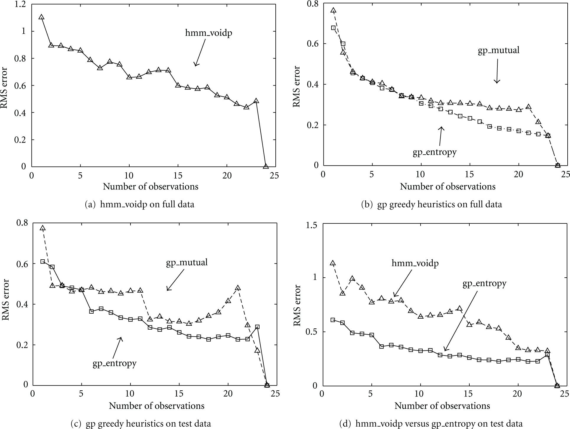
Prediction error versus number of selected observations on full dataset (a, b), and on test dataset (c, d), given by the HMM-based and GP-based selection approaches.

Figure 2

Mutual information gains on observations.

Figure 3

Mutual information values on observations.

The GP entropy-based selection is compared with the HMM-based selection on the test data in Figure 1(d). The GP-based approach beats the HMM-based approach in terms of predictive accuracy on the test data.

Figures 4(a)–4(c) examine how the erroneous observations affect these model-based selection approaches. In the figures, the circles and crosses denote the results, the dash and solid lines present the trends by doing regression based on the results. It shows that both GP based heuristic methods suffer big losses in predictive accuracy given the error-injected observations. However, the HMM-based approach shows a very robust performance with a little increased of the prediction errors.

Figure 4

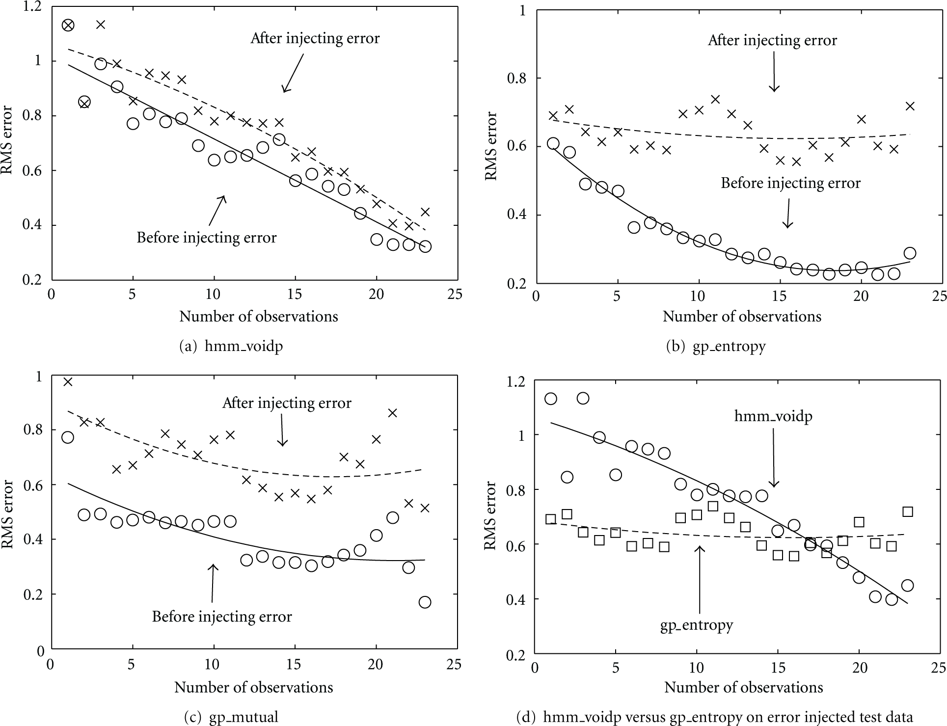
(a–c) Comparison of prediction errors on the original and error-injected test data by HMM-based selection, GP-based entropy heuristic, and GP-based mutual information heuristic selections, respectively; (d) comparing HMM-based selection against GP-based entropy heuristic selection on the test data with erroneous observations.

Despite both the GP-based heuristics perform poorly with erroneous observations, the mutual information heuristic is slightly more stable. In Figure 4(c), the two trend lines are parallel to each other whereas Figure 4(b) shows a big difference in performances by the entropy heuristic before and after the errors are injected into the observations.

The GP-based entropy heuristic is compared with the HMM-based selection under the erroneous observations because of its relatively lower prediction error over the mutual information heuristic. Figure 4(d) illustrates the result. It shows that the GP-based entropy method tends to maintain a constant error as the number of observations increases, meaning more observations do not help the predictive accuracy. Conversely, the HMM-based approach has a decreasing trend on predictive accuracy as more observations are added. After 16 observations the HMM-based selection method outperforms the GP-based method in terms of the RMS prediction errors.

The robustness against observation errors exhibited by the HMM-based selection approach is partly attributed to the conditional independence property provided inherently by the corresponding probabilistic chain graphical model. The observations on the chain graphical model cut the entire chain into smaller subchains, and the observations on one subchain will not directly affect the predictions on the other subchains. This property minimizes the effect caused by the erroneous observations. But for the GP-based approach, the predictions take all the observations directly into account, which therefore increases the chance of being affected by the errors in observations.

5. Conclusions

In this paper, we tackle the sensor scheduling problem by selecting a subset of time points to observe in order to make the most accurate predictions for the unobserved time points. We compare two model-based selection approaches, the probabilistic graphical model-based approach, particularly with HMM, and the Gaussian process model-based approach employing both entropy and mutual information greedy heuristics.

The results show that the GP-based approach performs better than the graphical model-based approach in terms of the predictive accuracy with accurate observations. But when small errors are injected into the observations, the GP-based selection method performs very poorly. In contrast, the graphical model-based approach demonstrates more robust and stable performance given the erroneous observations, and outperforms the GP-based approach when more observations are selected.

References

Dutta

Sustainable sensing for a smarter planet

XRDS 2011 17 14 20

George

E. I.

The Variable Selection Problem

Journal of the American Statistical Association 2000 95 452 1304 1308

2-s2.0-0442309436

Hastie

Tibshirani

Friedman

The Elements of Statistical Learning: Data Mining, Inference, and Prediction 2009 2nd

New York, NY, USA

Springer

Jordan

M. I.

Learning in Graphical Models 2001 2nd

Cambridge, Mass, USA

MIT Press

Krause

Guestrin

Optimal value of information in graphical models

Journal of Artificial Intelligence Research 2009 35 1 557 591

Shang

Shi

An improved algorithm for optimal subset selection in chain graphical models

Proceedings of the IEEE Congress on Evolutionary Computation (CEC '10)

2010

10.1109/CEC.2010.5586022

Rasmussen

C. E.

Williams

C. K. I.

Gaussian Processes for Machine Learning 2006

Cambridge, Mass, USA

MIT Press

Krause

Singh

Guestrin

Near-optimal sensor placements in Gaussian processes: theory, efficient algorithms and empirical studies

Journal of Machine Learning Research 2008 9 235 284

2-s2.0-41549146576

Zhuang

Shang

Shi

Model-based traffic prediction using sensor networks

Proceedings of the 5th IEEE Consumer Communications and Networking Conference (CCNC '08)

2008

136 140

10.1109/ccnc08.2007.38

10.

Caselton

W. F.

Zidek

J. V.

Optimal monitoring network designs

Statistics and Probability Letters 1984 2 4 223 227

2-s2.0-0001485154

11.

Vazirani

V. V.

Approximation Algorithms 2003 2nd

Berlin, Germany

Springer

12.

Krause

Guestrin

Optimal nonmyopic value of information in graphical models: efficient algorithms and theoretical limits

Proceedings of the 19th International Joint Conference on Artificial Intelligence (IJCAI '05)

2005

San Francisco, Calif, USA

Morgan Kaufmann Publishers

1339 1345

13.

Nemhauser

G. L.

Wolsey

L. A.

Fisher

M. L.

An analysis of approximations for maximizing submodular set functions

Mathematical Programming 1978 14 1 265 294

2-s2.0-0000095809

10.1007/BF01588971

14.

Deshpande

Guestrin

Madden

S. R.

Hellerstein

J. M.

Hong

Model-driven data acquisition in sensor networks

Proceedings of the 30th International Conference on Very Large Data Bases (VLDB '04)

2004

VLDB Endowment

588 599

Comparison of Probabilistic Chain Graphical Model-Based and Gaussian Process-Based Observation Selections for Wireless Sensor Scheduling

Abstract

1. Introduction

2. Probabilistic Graphical-Model-Based Observation Selection

Algorithm 1: Corrected VoIDP algorithm for optimizing observation selection on chain graphical models.

3. Gaussian Process-Based Observation Selection

3.1. The Entropy Heuristic

Algorithm 2: Greedy algorithm for maximizing entropy H ( 𝒜 ) .

3.2. The Mutual Information Heuristic

Algorithm 3: Greedy algorithm for maximizing mutual information gain M I ( 𝒜 ∪ y ) - M I ( 𝒜 ) using lazy evaluation.

4. Comparison Experiments

4.1. Experimental Setup

4.2. Results and Discussion

5. Conclusions

References

Algorithm 2: Greedy algorithm for maximizing entropy $H (𝒜)$ .

Algorithm 3: Greedy algorithm for maximizing mutual information gain $M I (𝒜 \cup y) - M I (𝒜)$ using lazy evaluation.