Performance Analysis of Distributed Incremental LMS Algorithm with Noisy Links

Abstract

Recently proposed distributed adaptive estimation algorithms for wireless sensor networks (WSNs) do not consider errors due to noisy links, which occur during the transmission of local estimates between sensors. In this paper, we study the effect of noisy links on the performance of distributed incremental least-mean-square (DILMS) algorithm for the case of Gaussian regressors. More specifically, we derive theoretical relations which explain how steady-state performance of DILMS algorithm (in terms of mean-square deviation (MSD), excess mean-square error (EMSE), and mean-square error (MSE)) is affected by noisy links. In our analysis, we use a spatial-temporal energy conservation argument to evaluate the steady-state performance of the individual nodes across the entire network. Our simulation results show that there is a good match between simulations and derived theoretical expressions. However, the important result is that unlike the ideal links case, the steady-state MSD, EMSE and MSE are not monotonically increasing functions of step size parameter when links are noisy. In addition, the optimal step size is found in a closed form for a special case which minimizes the steady-state values of MSD, EMSE, and MSE in each node.

1. Introduction

In many wireless sensor network applications, multiple displaced sensors are used to estimate and track an unknown parameter, for example, average temperature, level of water contaminants, or a target position [1, 2]. In general, parameter estimation in WSN can be solved by either a centralized approach or a decentralized approach [3]. In a centralized approach, the spatially distributed sensor send their locally processed data to a fusion center to form the final estimate [4–6]. As the number of nodes increases, centralized processing becomes computationally prohibitive, since it would require communications over longer range which leads to reduced battery life. On the other hand, in decentralized estimation, spatially displaced sensors provide local estimates by collaborating with other nodes in the network [7–9].

In some WSN applications, the parameter estimation task must be done whereas the statistical model for the underlying processes of interest is not available, or it changes over time. This issue motivated the development of special class of decentralized approaches known as distributed adaptive estimation schemes [10–14]. In these schemes, every node is equipped with local computing ability to derive a local estimate and share it with its predefined neighbors. Using cooperative processing in conjunction with adaptive filtering per node enables the entire network and also each individual node to track not only the variations of the environment but also the topology of the network.

Depending on the manner by which the nodes communicate with each other, they may be referred to as incremental algorithms or diffusion algorithms. In the incremental mode, a cyclic path through the network is required, and nodes communicate with neighbors within this path [10–12]. The given algorithms in [10–12] use different adaptive filter in their structure, such as LMS, recursive least-squares (RLS), and affine projection. When more communication and energy resources are available, a diffusion cooperative scheme can be applied where nodes communicate with all of their neighbors, and no cyclic path is required. Both LMS-based and RLS-based diffusion algorithms have been considered in the literature [13, 14]. In [15], we have considered the quantization effects on the steady-state performance of DILMS algorithm.

1.1. Problem Description

Analysis of distributed estimation algorithms in the presence of noisy links is an important physical layer issue which has been considered for different algorithms in the literature [16–21]. Nevertheless, this issue has not been considered in distributed adaptive estimation algorithms. Hence, in this paper, we study the performance of DILMS algorithm in a WNS with noisy links between sensors. The importance of such a study arises from the following facts:

• (i)

The WSN with noisy links is more realistic assumption than WSN with ideal links.

(ii)

The performance of distributed adaptive estimation algorithm (e.g., DILMS) can vary significantly when they are used in noisy links WSN, which makes it vital to analyze their performance.

Our aim in this paper is to derive some theoretical expressions that describe the steady-state performance of DILMS algorithm with noisy links. It must be noted that analyzing the DILMS algorithm in a WSN with noisy links is challenging task, since an adaptive network comprises a system of systems that processes data cooperatively in both time and space in presence of noisy links. To be more specific, the contributions of this paper are listed below.

1.2. Contributions

• (1)

  We show that the performance of distributed adaptive estimation algorithms drastically decreases when links are noisy.

• (2)

  We show that unlike the ideal link case [10], the steady-state MSD, EMSE, and MSE curves are not monotonically increasing functions of step size when links are noisy. This result is very important in real-world DILMS implementation and highlights the importance of our work.

• (3)

  The optimal step size is found in a closed form for a special case which minimizes the steady-state values of MSD, EMSE, and MSE in each sensor.

1.3. Paper Organization

The remainder of this paper is organized as follows: in Section 2, we introduce the DILMS algorithm. In Section 3, we present our analysis and explain some results of the derived theoretical results in Section 4. Simulation results are given in Section 5, and Finally, the conclusions are drawn in Section 6.

1.4. Notation

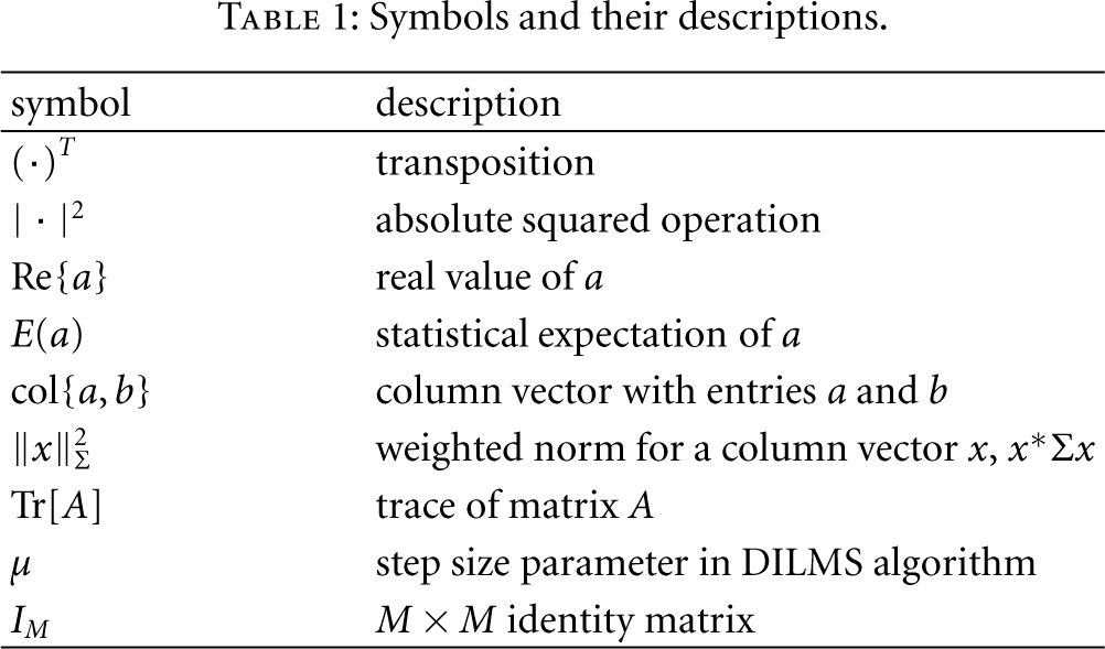
Throughout the paper, we adopt boldface letters for random quantities and normal font for nonrandom (deterministic) quantities. The “*” symbol is used for both complex conjugation for scalars and Hermitian transpose for matrices. The main symbols used in this paper are listed in Table 1.

Table 1

Symbols and their descriptions.

symbol	description
$(·{)}^T$	transposition
$|·{|}^2$	absolute squared operation
$\mathrm{Re}\{a\}$	real value of a
$E(a)$	statistical expectation of a
$\text{col}\{a,b\}$	column vector with entries a and b
$\parallel x{\parallel }_{\Sigma }^2$	weighted norm for a column vector x, $x^{*}\Sigma x$
$\mathrm{Tr}\hspace{0.17em}[A]$	trace of matrix A
μ	step size parameter in DILMS algorithm
$I_M$	$M\times M$ identity matrix

2. The DILMS Algorithm

Suppose that a WSN is deployed to estimate an unknown vector $w^o$ from measurements collected at N nodes in a network. Each node k has access to time realizations $\{d_k(i),u_{k,i}\}$ of zero-mean spatial data $\{{\mathbf{d}}_k,{\mathbf{u}}_k\}$ , where each ${\mathbf{d}}_k$ is a scalar measurement and each ${\mathbf{u}}_k$ is a $1\times M$ row regression vector. We collect the regression and measurement data into global matrices as

$\begin{array}{cc}\hfill \mathbf{U}& \triangleq \text{col}\left\{{\mathbf{u}}_1,{\mathbf{u}}_2,\dots ,{\mathbf{u}}_N\right\}\hspace{0.17em}\hspace{0.17em}\left(N\times M\right),\hfill \\ \hfill \mathbf{d}& \triangleq \text{col}\left\{{\mathbf{d}}_1,{\mathbf{d}}_2,\dots ,{\mathbf{d}}_N\right\}\hspace{0.17em}\hspace{0.17em}\left(N\times 1\right),\hfill \end{array}$

(1)

then the estimation problem is formulated as

$\begin{array}{c}\underset{w}{\min }\hspace{0.17em}J\left(w\right),\hspace{1em}\text{where}\hspace{0.17em}\hspace{0.17em}J\left(w\right)=E\left({\Vert \mathbf{d}-\mathbf{U}w\Vert }^2\right).\end{array}$

(2)

In the appendix, we introduce a motivating application where an estimation problem (2) arises. The optimal solution $w^o$ is given by [10]

$\begin{array}{c}{R}_{du}=R_u{w}^o,\end{array}$

(3)

where $R_{du}=E({\mathbf{U}}^{*}\mathbf{d})$ and $R_u=E({\mathbf{U}}^{*}\mathbf{U})$ . Note that the cost function (2) can be decomposed as [10]

$\begin{array}{c}J\left(w\right)={\displaystyle \sum }_{k=1}^N{J}_k\left(w\right),\hspace{1em}\text{where}\hspace{0.17em}\hspace{0.17em}{J}_k\left(w\right)=E\left({\left|{\mathbf{d}}_k-{\mathbf{u}}_{k}w\right|}^2\right).\end{array}$

(4)

Using this property, in [10], a distributed incremental LMS strategy with a cyclic estimation structure is proposed, as follows:

$\begin{array}{cc}\hfill & {\mathbf{\psi }}_0^{\left(i\right)}⟵{\mathbf{w}}_{i-1},\hfill \\ \hfill & {\mathbf{\psi }}_k^{\left(i\right)}=\underset{k=\mathrm{1,2},\dots ,N}{{\mathbf{\psi }}_{k-1}^{\left(i\right)}}+{\mu }_k{\mathbf{u}}_{k,i}^{*}\left[{\mathbf{d}}_k\left(i\right)-{\mathbf{u}}_{k,i}{\mathbf{\psi }}_{k-1}^{\left(i\right)}\right],\hfill \\ \hfill & {\mathbf{w}}_i⟵{\mathbf{\psi }}_N^{\left(i\right)},\hfill \end{array}$

(5)

where ${\mathbf{\psi }}_k^{(i)}$ indicates the local estimate at the node k and time i and ${\mathbf{w}}_i$ indicates the overall estimate at iteration i. For each time i, each node utilizes the local data ${\mathbf{d}}_k(i),{\mathbf{u}}_{k,i}$ and ${\mathbf{\psi }}_{k-1}^{(i)}$ received from the node $k-1$ to obtain ${\mathbf{\psi }}_k^{(i)}$ . At the end of this cycle, ${\mathbf{\psi }}_N^{(i)}$ is employed as both the global estimate ${\mathbf{w}}_i$ and the initial condition for the next time instant. Note that to implement the DILMS, the time realizations $\{d_k(i),u_{k,i}\}$ are used. The update equation for DILMS in noisy link condition changes to

$\begin{array}{c}{\mathbf{\psi }}_k^{\left(i\right)}={\mathbf{\psi }}_{k-1}^{\left(i\right)}+{\mathbf{q}}_{k,i}+{\mu }_k{\mathbf{u}}_{k,i}^{*}\left[{\mathbf{d}}_k\left(i\right)-{\mathbf{u}}_{k,i}\left({\mathbf{\psi }}_{k-1}^{\left(i\right)}+{\mathbf{q}}_{k,i}\right)\right],\end{array}$

(6)

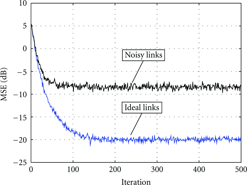
where the $M\times 1$ vector ${\mathbf{q}}_{k,i}$ is the channel noise term between sensor k and $k-1$ which is assumed to be additive with zero mean and covariance matrix $Q_k$ . No distributional assumptions are required on the noise sequence. To show the effect of noisy links on the performance of DILMS algorithms, we consider a network with $N=20$ nodes. The observation noise has a variance of ${\sigma }_{v,k}^2=10^{-2}$ , and also we assume $Q_k=10^{-3}{I}_M$ for channel noise. The curves are obtained by averaging over 300 experiments with $\mu =0.001$ (see Figure 1). As it is clear from Figure 1, the performance of DILMS algorithms drastically decreases when links are noisy.

Figure 1

The effect of noisy links on the performance of DILMS algorithm.

3. Performance Analysis

3.1. Data Model and Assumptions

In order to pursue the performance analysis, we will rely on the energy conservation approach of [10, 22]. Also, to carry out the performance analysis, we first need to assume a model for the data as is commonly done in the literature of adaptive algorithms. In the subsequent analysis, the following assumptions will be considered.

• (A.1)

The desired unknown vector $w^o$ relates to the $\{{\mathbf{d}}_k(i),{\mathbf{u}}_{k,i}\}$ via

$\begin{array}{c}{\mathbf{d}}_k\left(i\right)={\mathbf{u}}_{k,i}{w}^o+{\mathbf{v}}_k\left(i\right),\end{array}$

(7)

where ${\mathbf{v}}_k(i)$ is white noise term with variance ${\sigma }_{v,k}^2$ and is independent of $\{{\mathbf{d}}_l(j),{\mathbf{u}}_{l,j}\}$ for all $l,j$ .

(A.2)

${\mathbf{u}}_{k,i}$ is independent of ${\mathbf{u}}_{l,i}$ for $k\ne l$ .

(A.3)

${\mathbf{u}}_{k,i}$ is independent of ${\mathbf{u}}_{k,j}$ for $i\ne j$ .

(A.4)

${\mathbf{q}}_{k,i}$ is independent of $\{{\mathbf{u}}_{l,j},{\mathbf{v}}_l(j),{\mathbf{q}}_{l,j}\}$ for all $l,j$ .

3.2. Weighted Energy Conservation Relation

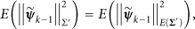
In steady-state analysis, we are interested in evaluating the MSD, EMSE, and MSE for every node k which are defined as

$\begin{array}{cc}\hfill {\eta }_k& \triangleq E\left({\Vert {\tilde{\mathbf{\psi }}}_{k-1}^{\left(\infty \right)}\Vert }^2\right)=E\left({\Vert {\tilde{\mathbf{\psi }}}_{k-1}^{\left(\infty \right)}\Vert }_I^2\right)\hspace{1em}\left(\text{MSD}\right),\hfill \\ \hfill {\zeta }_k& \triangleq E\left({\left|{\mathbf{e}}_{a,k}\left(\infty \right)\right|}^2\right)=E\left({\Vert {\tilde{\mathbf{\psi }}}_{k-1}^{\left(\infty \right)}\Vert }_{R_{u,k}}^2\right)\hspace{1em}\left(\text{EMSE}\right),\hfill \\ \hfill {\xi }_k& \triangleq E\left({\left|{\mathbf{e}}_k\left(\infty \right)\right|}^2\right)={\zeta }_k+{\sigma }_{v,k}^2\hspace{1em}\left(\text{MSE}\right),\hfill \end{array}$

(8)

where ${\mathbf{e}}_k(i)\triangleq {\mathbf{d}}_k(i)-{\mathbf{u}}_{k,i}{\mathbf{\psi }}_{k-1}^{(i)}$ , ${\mathbf{e}}_{a,k}(i)\triangleq {\mathbf{u}}_{k,i}{\tilde{\mathbf{\psi }}}_{k-1}^{(i)}$ , and ${\tilde{\mathbf{\psi }}}_k^{(i)}\triangleq w^o-{\mathbf{\psi }}_k^{(i)}$ . Note that due to incremental cooperation (cyclic path), for $k=1$ we use $k-1=N$ in (8). We further define the weighted a priori and a posteriori local errors for each node k as follows:

$\begin{array}{c}{\mathbf{e}}_{a,k}^{\Sigma }\left(i\right)={\mathbf{u}}_{k,i}\Sigma {\tilde{\mathbf{\psi }}}_{k-1}^{\left(i\right)},\hspace{1em}\hspace{1em}{\mathbf{e}}_{p,k}^{\Sigma }\left(i\right)={\mathbf{u}}_{k,i}\Sigma {\tilde{\mathbf{\psi }}}_k^{\left(i\right)}.\end{array}$

(9)

Using (6) and the definition of ${\mathbf{e}}_k(i)$ , we have

$\begin{array}{c}{\mathbf{\psi }}_k^{\left(i\right)}={\mathbf{\psi }}_{k-1}^{\left(i\right)}+{\mu }_k{\mathbf{u}}_{k,i}^{*}{\mathbf{e}}_k\left(i\right)+{\mathbf{q}}_{k,i}-{\mu }_k{\mathbf{u}}_{k,i}^{*}{\mathbf{u}}_{k,i}{\mathbf{q}}_{k,i}.\end{array}$

(10)

By subtracting $w^o$ from both sides of (10), we get

$\begin{array}{c}{\tilde{\mathbf{\psi }}}_k^{\left(i\right)}={\tilde{\mathbf{\psi }}}_{k-1}^{\left(i\right)}-{\mu }_k{\mathbf{u}}_{k,i}^{*}{\mathbf{e}}_k\left(i\right)-{\mathbf{q}}_{k,i}+{\mu }_k{\mathbf{u}}_{k,i}^{*}{\mathbf{u}}_{k,i}{\mathbf{q}}_{k,i}.\end{array}$

(11)

Multiplying the previous equation from left by ${\mathbf{u}}_{k,i}\Sigma$ and using the definitions in (9), we have

$\begin{array}{cc}\hfill {\mathbf{e}}_{p,k}^{\Sigma }\left(i\right)& ={\mathbf{e}}_{a,k}^{\Sigma }\left(i\right)-{\mu }_k{\Vert {\mathbf{u}}_{k,i}\Vert }_{\Sigma }^2{\mathbf{e}}_k\left(i\right)-{\mathbf{u}}_{k,i}\Sigma {\mathbf{q}}_{k,i}\hfill \\ \hfill & \hspace{1em}+{\mu }_k{\Vert {\mathbf{u}}_{k,i}\Vert }_{\Sigma }^2{\mathbf{u}}_{k,i}{\mathbf{q}}_{k,i}.\hfill \end{array}$

(12)

By replacing the ${\mathbf{e}}_k(i)$ from (11) and equating the weighted norm of both sides of the resultant equation, we arrive to the following relation:

$\begin{array}{cc}\hfill & {\Vert {\tilde{\mathbf{\psi }}}_k^{\left(i\right)}\Vert }_{\Sigma }^2+\frac{{\left|{\mathbf{e}}_{a,k}^{\Sigma }\left(i\right)\right|}^2}{{\Vert {\mathbf{u}}_{k,i}\Vert }_{\Sigma }^2}\hfill \\ \hfill & \hspace{1em}={\Vert {\tilde{\mathbf{\psi }}}_{k-1}^{\left(i\right)}\Vert }_{\Sigma }^2+\frac{{\left|{\mathbf{e}}_{p,k}^{\Sigma }\left(i\right)\right|}^2}{{\Vert {\mathbf{u}}_{k,i}\Vert }_{\Sigma }^2}+{\Vert {\mathbf{q}}_{k,i}\Vert }_{\Sigma }^2-2\mathrm{Re}\left\{{\tilde{\mathbf{\psi }}}_{k-1}^{\left(i\right)*}\Sigma {\mathbf{q}}_{k,i}\right\}\hfill \\ \hfill & \hspace{1em}\hspace{1em}+2\mathrm{Re}\left\{\frac{{\tilde{\mathbf{\psi }}}_{k-1}^{\left(i\right)*}\Sigma {\mathbf{u}}_{k,i}^{*}{\mathbf{u}}_{k,i}\Sigma {\mathbf{q}}_{k,i}}{{\Vert {\mathbf{u}}_{k,i}\Vert }_{\Sigma }^2}\right\}-\frac{{\mathbf{q}}_{k,i}^{*}\Sigma {\mathbf{u}}_{k,i}^{*}{\mathbf{u}}_{k,i}\Sigma {\mathbf{q}}_{k,i}}{\parallel {\mathbf{u}}_{k,i}{\parallel }_{\Sigma }^2}.\hfill \end{array}$

(13)

We find from (13) that the cross terms are canceled out. Equation (13) is a space-time version of the weighted energy conservation relation used in [10] in the context of regular adaptive implementations.

3.3. Weighted Variance Relation

In this section, we use the energy conservation relation to evaluate the steady-state performance of the DILMS algorithm in every node when the links between nodes are noisy. To this aim, we need to have a recursive equation for ${\parallel {\tilde{\mathbf{\psi }}}_k^{(i)}\parallel }_{\Sigma }^2$ . To obtain such a recursion we replace ${\mathbf{e}}_{p,k}^{\Sigma }(i)$ from (12) into (13) to get

$\begin{array}{cc}\hfill {\Vert {\tilde{\mathbf{\psi }}}_k\Vert }_{\Sigma }^2& ={\Vert {\tilde{\mathbf{\psi }}}_{k-1}\Vert }_{\Sigma }^2-2\mathrm{Re}\left\{{\tilde{\mathbf{\psi }}}_{k-1}^{*}\Sigma {\mathbf{q}}_k\right\}+{\Vert {\mathbf{q}}_k\Vert }_{\Sigma }^2\hfill \\ \hfill & \hspace{1em}+2{\mu }_k\mathrm{Re}\left\{{\mathbf{e}}_{a,k}^{\Sigma *}{\mathbf{u}}_k{\mathbf{q}}_k\right\}-{\mu }_k{\mathbf{q}}_k^{*}\Sigma {\mathbf{u}}_k^{*}{\mathbf{u}}_k{\mathbf{q}}_k\hfill \\ \hfill & \hspace{1em}-{\mu }_k{\mathbf{q}}_k^{*}{\mathbf{u}}_k^{*}{\mathbf{u}}_k\Sigma {\mathbf{q}}_k+{\mu }_k^2\parallel {\mathbf{u}}_k{\parallel }_{\Sigma }^2{\mathbf{q}}_k^{*}{\mathbf{u}}_k^{*}{\mathbf{u}}_k{\mathbf{q}}_k\hfill \\ \hfill & \hspace{1em}-{\mu }_k{\mathbf{e}}_{a,k}^{\Sigma *}{\mathbf{e}}_k-{\mu }_k{\mathbf{e}}_k^{*}{\mathbf{e}}_{a,k}^{\Sigma }+{\mu }_k^2{\Vert {\mathbf{u}}_k\Vert }_{\Sigma }^2{\left|{\mathbf{e}}_k\right|}^2\hfill \\ \hfill & \hspace{1em}+{\mu }_k{\mathbf{e}}_k^{*}{\mathbf{u}}_k\Sigma {\mathbf{q}}_k-{\mu }_k^2{\Vert {\mathbf{u}}_k\Vert }_{\Sigma }^2{\mathbf{e}}_k^{*}{\mathbf{u}}_k{\mathbf{q}}_k\hfill \\ \hfill & \hspace{1em}+{\mu }_k{\mathbf{q}}_k^{*}\Sigma {\mathbf{u}}_k^{*}{\mathbf{e}}_k-{\mu }_k^2{\Vert {\mathbf{u}}_k\Vert }_{\Sigma }^2{\mathbf{q}}_k^{*}{\mathbf{u}}_k^{*}{\mathbf{e}}_k.\hfill \end{array}$

(14)

We have dropped the time index i for compactness of notation. Now, we can relate the ${\mathbf{e}}_k$ to ${\mathbf{e}}_{a,k}$ via

$\begin{array}{c}{\mathbf{e}}_k={\mathbf{e}}_{a,k}+{\mathbf{v}}_k.\end{array}$

(15)

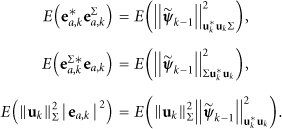
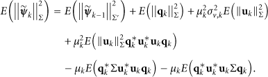
If we replace (15) into (14), take expectation of both sides, and use assumptions (A.1)–(A.4), we obtain

$\begin{array}{cc}\hfill E\left({\Vert {\tilde{\mathbf{\psi }}}_k\Vert }_{\Sigma }^2\right)& =E(\parallel {\tilde{\mathbf{\psi }}}_{k-1}{\parallel }_{\Sigma }^2)+E\left({\Vert {\mathbf{q}}_k\Vert }_{\Sigma }^2\right)\hfill \\ \hfill & \hspace{1em}-{\mu }_{k}E\left({\mathbf{e}}_{a,k}^{\Sigma *}{\mathbf{e}}_{a,k}\right)-{\mu }_{k}E\left({\mathbf{e}}_{a,k}^{*}{\mathbf{e}}_{a,k}^{\Sigma }\right)\hfill \\ \hfill & \hspace{1em}+{\mu }_k^{2}E\left({\Vert {\mathbf{u}}_k\Vert }_{\Sigma }^2{\left|{\mathbf{e}}_{a,k}\right|}^2\right)+{\mu }_k^2{\sigma }_{v,k}^{2}E\left({\Vert {\mathbf{u}}_k\Vert }_{\Sigma }^2\right)\hfill \\ \hfill & \hspace{1em}+{\mu }_k^{2}E\left({\Vert {\mathbf{u}}_k\Vert }_{\Sigma }^2{\mathbf{q}}_k^{*}{\mathbf{u}}_k^{*}{\mathbf{u}}_k{\mathbf{q}}_k\right)\hfill \\ \hfill & \hspace{1em}-{\mu }_{k}E\left({\mathbf{q}}_k^{*}\Sigma {\mathbf{u}}_k^{*}{\mathbf{u}}_k{\mathbf{q}}_k\right)-{\mu }_{k}E\left({\mathbf{q}}_k^{*}{\mathbf{u}}_k^{*}{\mathbf{u}}_k\Sigma {\mathbf{q}}_k\right).\hfill \end{array}$

(16)

By considering the error definitions ${\mathbf{e}}_{a,k}^{\Sigma }$ and ${\mathbf{e}}_{a,k}$ , we can obtain the following relations:

$\begin{array}{cc}\hfill E\left({\mathbf{e}}_{a,k}^{*}{\mathbf{e}}_{a,k}^{\Sigma }\right)& =E\left({\Vert {\tilde{\mathbf{\psi }}}_{k-1}\Vert }_{{\mathbf{u}}_k^{*}{\mathbf{u}}_k\Sigma }^2\right),\hfill \\ \hfill E\left({\mathbf{e}}_{a,k}^{\Sigma *}{\mathbf{e}}_{a,k}\right)& =E\left({\Vert {\tilde{\mathbf{\psi }}}_{k-1}\Vert }_{\Sigma {\mathbf{u}}_k^{*}{\mathbf{u}}_k}^2\right),\hfill \\ \hfill E\left({\Vert {\mathbf{u}}_k\Vert }_{\Sigma }^2{\left|{\mathbf{e}}_{a,k}\right|}^2\right)& =E\left({\Vert {\mathbf{u}}_k\Vert }_{\Sigma }^2{\Vert {\tilde{\mathbf{\psi }}}_{k-1}\Vert }_{{\mathbf{u}}_k^{*}{\mathbf{u}}_k}^2\right).\hfill \end{array}$

(17)

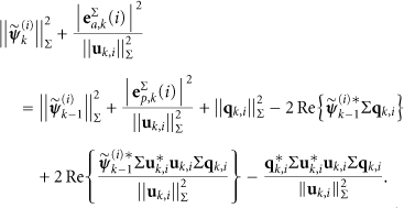
Using the property ${\parallel x\parallel }_A^2+{\parallel x\parallel }_B^2={\parallel x\parallel }_{A+B}^2$ and (17), we can expand (16) as

$\begin{array}{cc}\hfill E\left({\Vert {\tilde{\mathbf{\psi }}}_k\Vert }_{\Sigma }^2\right)& =E\left({\Vert {\tilde{\mathbf{\psi }}}_{k-1}\Vert }_{{𝚺}^{\prime }}^2\right)+E\left({\Vert {\mathbf{q}}_k\Vert }_{\Sigma }^2\right)+{\mu }_k^2{\sigma }_{v,k}^{2}E\left({\Vert {\mathbf{u}}_k\Vert }_{\Sigma }^2\right)\hfill \\ \hfill & \hspace{1em}+{\mu }_k^{2}E\left({\Vert {\mathbf{u}}_k\Vert }_{\Sigma }^2{\mathbf{q}}_k^{*}{\mathbf{u}}_k^{*}{\mathbf{u}}_k{\mathbf{q}}_k\right)\hfill \\ \hfill & \hspace{1em}-{\mu }_{k}E\left({\mathbf{q}}_k^{*}\Sigma {\mathbf{u}}_k^{*}{\mathbf{u}}_k{\mathbf{q}}_k\right)-{\mu }_{k}E\left({\mathbf{q}}_k^{*}{\mathbf{u}}_k^{*}{\mathbf{u}}_k\Sigma {\mathbf{q}}_k\right),\hfill \end{array}$

(18)

where in (18), we have

$\begin{array}{c}{𝚺}^{\prime }\triangleq \Sigma -{\mu }_k\Sigma {\mathbf{u}}_k^{*}{\mathbf{u}}_k-{\mu }_k{\mathbf{u}}_k^{*}{\mathbf{u}}_k\Sigma +{\mu }_k^2{\Vert {\mathbf{u}}_k\Vert }_{\Sigma }^2{\mathbf{u}}_k^{*}{\mathbf{u}}_k.\end{array}$

(19)

Invoking the independence of the regression data $\{{\mathbf{u}}_k\}$ allows us to write

$\begin{array}{c}E\left({\Vert {\tilde{\mathbf{\psi }}}_{k-1}\Vert }_{{\Sigma }^{\prime }}^2\right)=E\left({\Vert {\tilde{\mathbf{\psi }}}_{k-1}\Vert }_{E\left({𝚺}^{\prime }\right)}^2\right),\hspace{0.17em}\hspace{0.17em}\end{array}$

(20)

so that (18) becomes

$\begin{array}{cc}\hfill E\left({\Vert {\tilde{\mathbf{\psi }}}_k\Vert }_{\Sigma }^2\right)& =E\left({\Vert {\tilde{\mathbf{\psi }}}_{k-1}\Vert }_{{\Sigma }^{\prime }}^2\right)+E\left({\Vert {\mathbf{q}}_k\Vert }_{\Sigma }^2\right)+{\mu }_k^2{\sigma }_{v,k}^{2}E\left({\Vert {\mathbf{u}}_k\Vert }_{\Sigma }^2\right)\hfill \\ \hfill & \hspace{1em}+{\mu }_k^{2}E\left({\Vert {\mathbf{u}}_k\Vert }_{\Sigma }^2{\mathbf{q}}_k^{*}{\mathbf{u}}_k^{*}{\mathbf{u}}_k{\mathbf{q}}_k\right)\hfill \\ \hfill & \hspace{1em}-{\mu }_{k}E\left({\mathbf{q}}_k^{*}\Sigma {\mathbf{u}}_k^{*}{\mathbf{u}}_k{\mathbf{q}}_k\right)-{\mu }_{k}E\left({\mathbf{q}}_k^{*}{\mathbf{u}}_k^{*}{\mathbf{u}}_k\Sigma {\mathbf{q}}_k\right).\hfill \end{array}$

(21)

Note that in (21), ${\Sigma }^{\prime }$ is a deterministic matrix as

$\begin{array}{c}{\Sigma }^{\prime }\triangleq \Sigma -{\mu }_{k}E\left(\Sigma {\mathbf{u}}_k^{*}{\mathbf{u}}_k+{\mathbf{u}}_k^{*}{\mathbf{u}}_k\Sigma \right)+{\mu }_k^{2}E\left({\Vert {\mathbf{u}}_k\Vert }_{\Sigma }^2{\mathbf{u}}_k^{*}{\mathbf{u}}_k\right).\end{array}$

(22)

Recursion (21) is a variance relation that can be used to infer the steady-state performance at every node k. Note that ${\Sigma }^{\prime }$ is solely regressors dependent and, therefore, decoupled from the weight error vector. For simplicity, in this work, we consider the following assumption.

• (A.5)

  The regressors $\{{\mathbf{u}}_k\}$ arise from a source with circular Gaussian distribution with covariance matrix $R_{u,k}$ .

We introduce the eigndecomposition $R_{u,k}=U_k{\mathrm{\Lambda }}_k{U}_k^{*}$ , where ${\mathrm{\Lambda }}_k$ is a diagonal matrix with the eigenvalues of $R_{u,k}$ and $U_k$ is unitary, that is, $U_k{U}_k^{*}=U_k^{*}{U}_k=I$ . Define the transformed quantities

$\begin{array}{c}{\bar{\mathbf{\psi }}}_k\triangleq U_k^{*}{\tilde{\mathbf{\psi }}}_k,\hspace{0.17em}\hspace{0.17em}\hspace{1em}\hspace{1em}{\bar{\mathbf{\psi }}}_{k-1}\triangleq U_k^{*}{\tilde{\mathbf{\psi }}}_{k-1},\hspace{1em}\hspace{1em}{\bar{\mathbf{u}}}_k\triangleq {\mathbf{u}}_k{U}_k,\\ {\bar{\mathbf{q}}}_k\triangleq U_k^{*}{\mathbf{q}}_k,\hspace{1em}\hspace{1em}\bar{\Sigma }\triangleq U_k^{*}\Sigma U_k,\hspace{1em}\hspace{1em}{\bar{\Sigma }}^{\prime }\triangleq U_k^{*}{\Sigma }^{\prime }{U}_k.\end{array}$

(23)

Using the above definitions, (21) and (22) can be rewritten in the equivalent forms

$\begin{array}{c}\begin{array}{cc}E\left({\Vert {\bar{\mathbf{\psi }}}_k\Vert }_{\bar{\Sigma }}^2\right)\hfill & =E\left({\Vert {\bar{\mathbf{\psi }}}_{k-1}\Vert }_{{\bar{\Sigma }}^{\prime }}^2\right)+E\left({\Vert {\bar{\mathbf{q}}}_k\Vert }_{\bar{\Sigma }}^2\right)\hfill \\ \hfill & \hspace{1em}+{\mu }_k^2{\sigma }_{v,k}^{2}E\left({\Vert {\bar{\mathbf{u}}}_k\Vert }_{\bar{\Sigma }}^2\right)+{\mu }_k^{2}E\left({\Vert {\bar{\mathbf{u}}}_k\Vert }_{\bar{\Sigma }}^2{\bar{\mathbf{q}}}_k^{*}{\bar{\mathbf{u}}}_k^{*}{\bar{\mathbf{u}}}_k{\bar{\mathbf{q}}}_k\right)\hspace{0.17em}\hspace{0.17em}\hfill \\ \hfill & \hspace{1em}-{\mu }_{k}E\left({\bar{\mathbf{q}}}_k^{*}\bar{\Sigma }{\bar{\mathbf{u}}}_k^{*}{\bar{\mathbf{u}}}_k{\bar{\mathbf{q}}}_k\right)-{\mu }_{k}E\left({\bar{\mathbf{q}}}_k^{*}{\bar{\mathbf{u}}}_k^{*}{\bar{\mathbf{u}}}_k\bar{\Sigma }{\bar{\mathbf{q}}}_k\right),\hfill \end{array}\\ {\bar{\Sigma }}^{\prime }=\bar{\Sigma }-{\mu }_{k}E\left(\bar{\Sigma }{\bar{\mathbf{u}}}_k^{*}{\bar{\mathbf{u}}}_k+{\bar{\mathbf{u}}}_k^{*}{\bar{\mathbf{u}}}_k\bar{\Sigma }\right)+{\mu }_k^{2}E\left({\Vert {\bar{\mathbf{u}}}_k\Vert }_{\bar{\Sigma }}^2{\bar{\mathbf{u}}}_k^{*}{\bar{\mathbf{u}}}_k\right).\end{array}$

(24)

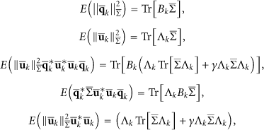
To proceed, we need to evaluate the moments in (24) as follows:

$\begin{array}{c}\begin{array}{c}E\left({\Vert {\bar{\mathbf{q}}}_k\Vert }_{\bar{\Sigma }}^2\right)=\mathrm{Tr}\left[B_k\bar{\Sigma }\right],\end{array}\\ E\left({\Vert {\bar{\mathbf{u}}}_k\Vert }_{\bar{\Sigma }}^2\right)=\mathrm{Tr}\left[{\Lambda }_k\bar{\Sigma }\right],\\ E\left({\Vert {\bar{\mathbf{u}}}_k\Vert }_{\bar{\Sigma }}^2{\bar{\mathbf{q}}}_k^{*}{\bar{\mathbf{u}}}_k^{*}{\bar{\mathbf{u}}}_k{\bar{\mathbf{q}}}_k\right)=\mathrm{Tr}\left[B_k\left({\Lambda }_k\mathrm{Tr}\left[\bar{\Sigma }{\Lambda }_k\right]+\gamma {\Lambda }_k\bar{\Sigma }{\Lambda }_k\right)\right],\\ E\left({\bar{\mathbf{q}}}_k^{*}\bar{\Sigma }{\bar{\mathbf{u}}}_k^{*}{\bar{\mathbf{u}}}_k{\bar{\mathbf{q}}}_k\right)=\mathrm{Tr}\left[{\Lambda }_k{B}_k\bar{\Sigma }\right],\\ E\left({\Vert {\bar{\mathbf{u}}}_k\Vert }_{\bar{\Sigma }}^2{\bar{\mathbf{u}}}_k^{*}{\bar{\mathbf{u}}}_k\right)=\left({\Lambda }_k\mathrm{Tr}\left[\bar{\Sigma }{\Lambda }_k\right]+\gamma {\Lambda }_k\bar{\Sigma }{\Lambda }_k\right),\end{array}$

(25)

where $B_k=U_k^{*}{Q}_k{U}_k$ and $\gamma =1$ for circular complex data and $\gamma =2$ for real data. Replacing these moments, (24) can be written as

$\begin{array}{cc}\hfill E\left({\Vert {\bar{\mathbf{\psi }}}_k\Vert }_{\bar{\Sigma }}^2\right)& =E\left({\Vert {\bar{\mathbf{\psi }}}_{k-1}\Vert }_{{\bar{\Sigma }}^{\prime }}^2\right)+\mathrm{Tr}\left[B_k\bar{\Sigma }\right]+{\mu }_k^2{\sigma }_{v,k}^2\mathrm{Tr}\left[{\Lambda }_k\bar{\Sigma }\right]\hfill \\ \hfill & \hspace{1em}+{\mu }_k^2\mathrm{Tr}\left[B_k\left({\Lambda }_k\mathrm{Tr}\left[\bar{\Sigma }{\Lambda }_k\right]+\gamma {\Lambda }_k\bar{\Sigma }{\Lambda }_k\right)\right]\hfill \\ \hfill & \hspace{1em}-2{\mu }_k\mathrm{Tr}\left[{\Lambda }_k{B}_k\bar{\Sigma }\right],\hfill \end{array}$

(26)

$\begin{array}{cc}\hfill {\bar{\Sigma }}^{\prime }& =\bar{\Sigma }-{\mu }_k\left(\bar{\Sigma }{\Lambda }_k+{\Lambda }_k\bar{\Sigma }\right)\hfill \\ \hfill & \hspace{1em}+{\mu }_k^2\left({\Lambda }_k\mathrm{Tr}\left[\bar{\Sigma }{\Lambda }_k\right]+\gamma {\Lambda }_k\bar{\Sigma }{\Lambda }_k\right).\hfill \end{array}$

(27)

Note from (27) that choosing $\bar{\Sigma }$ to be diagonal, ${\bar{\Sigma }}^{\prime }$ will be diagonal as well, suggesting a more compact notation. Thus, we introduce the $M\times 1$ column vectors

$\begin{array}{c}\bar{\sigma }\stackrel{\Delta }{=}\mathrm{diag}\left\{\bar{\Sigma }\right\},\hspace{1em}\hspace{1em}{\bar{\sigma }}^{\prime }\stackrel{\Delta }{=}\mathrm{diag}\left\{{\bar{\Sigma }}^{\prime }\right\},\hspace{1em}\hspace{1em}{\lambda }_k\stackrel{\Delta }{=}\mathrm{diag}\left\{{\Lambda }_k\right\},\end{array}$

(28)

where the $\mathrm{diag}\hspace{0.17em}\{\}$ notation will be used in two ways: $\lambda =\mathrm{diag}\hspace{0.17em}\{\mathrm{\Lambda }\}$ is a column vector containing the main diagonal of $\mathrm{\Lambda }$ , and $\mathrm{\Lambda }=\mathrm{diag}\hspace{0.17em}\{\lambda \}$ is a diagonal matrix whose entries are those of the vector λ. Therefore, using the diagonal notation, we obtain the following linear relation between the corresponding vectors $\{\bar{\sigma },{\bar{\sigma }}^{\prime }\}$ :

$\begin{array}{c}{\bar{\sigma }}^{\prime }={\bar{F}}_k\bar{\sigma },\end{array}$

(29)

where ${\bar{F}}_k$ is a $M\times M$ matrix that includes statistics of local data and given by

$\begin{array}{c}{\bar{F}}_k\stackrel{\Delta }{=}I-2{\mu }_k{\Lambda }_k+\gamma {\mu }_k^2{\Lambda }_k^2+{\mu }_k^2{\lambda }_k{\lambda }_k^T.\end{array}$

(30)

As a result, (26) becomes

$\begin{array}{c}E\left({\Vert {\bar{\mathbf{\psi }}}_k\Vert }_{\mathrm{diag}\left\{\bar{\sigma }\right\}}^2\right)=E\left({\Vert {\bar{\mathbf{\psi }}}_{k-1}\Vert }_{\mathrm{diag}\left\{{\bar{F}}_k\bar{\sigma }\right\}}^2\right)+g_k\bar{\sigma },\end{array}$

(31)

where $g_k$ is a row vector as

$\begin{array}{c}{g}_k\triangleq {\mu }_k^2{\sigma }_{v,k}^2{\lambda }_k^T+{\left(\mathrm{diag}\left\{B_k\right\}\right)}^T\left[I+{\mu }_k^2{\lambda }_k{\lambda }_k^T+\gamma {\mu }_k^2{\Lambda }_k^2-2{\mu }_k{\Lambda }_k\right].\end{array}$

(32)

Using (30), $g_k$ can be rewritten in a more compact form as

$\begin{array}{c}{g}_k={\mu }_k^2{\sigma }_{v,k}^2{\lambda }_k^T+{\left(\mathrm{diag}\left\{B_k\right\}\right)}^T{\bar{F}}_k.\end{array}$

(33)

For the sake of clarity, we reintroduce the time index i but drop the $\mathrm{diag}\hspace{0.17em}\{\}$ notation from the subscripts in (31) for compactness. Expression (31) becomes

$\begin{array}{c}E\left({\Vert {\bar{\mathbf{\psi }}}_k^{\left(i\right)}\Vert }_{{\bar{\sigma }}_k}^2\right)=E\left({\Vert {\bar{\mathbf{\psi }}}_{k-1}^{\left(i\right)}\Vert }_{{\bar{F}}_k{\bar{\sigma }}_k}^2\right)+g_k{\bar{\sigma }}_k.\end{array}$

(34)

We replaced $\{\bar{\sigma },{\bar{\sigma }}^{\prime }\}$ by $\{{\bar{\sigma }}_k,{\bar{\sigma }}_k^{\prime }\}$ in order to indicate that the weighting matrix can be node dependent.

3.4. Steady-State Behavior

By comparing (34) with the similar equation for DILMS algorithm with ideal links (i.e., equation (55) in [10]), we can conclude that the desired steady-state MSD, EMSE, and MSE for DILMS algorithm with noisy links at node k can be expressed as

$\begin{array}{c}{\eta }_k=a_k{\left(I-{\Pi }_{k,1}\right)}^{-1}r,\hspace{0.17em}\hspace{0.17em}\hspace{1em}\left(\text{MSD}\right),\end{array}$

(35)

$\begin{array}{c}{\zeta }_k=a_k{\left(I-{\Pi }_{k,1}\right)}^{-1}{\lambda }_k,\hspace{1em}\left(\text{EMSE}\right),\end{array}$

(36)

$\begin{array}{c}{\xi }_k={\zeta }_k+{\sigma }_{v,k}^2,\hspace{1em}\left(\text{MSE}\right),\end{array}$

(37)

where

$\begin{array}{c}{\Pi }_{k,l}\triangleq {\bar{F}}_{k+l-1}{\bar{F}}_{k+l}\cdots {\bar{F}}_N{\bar{F}}_1\cdots {\bar{F}}_{k-1},\hspace{1em}l=1,\dots ,N,\end{array}$

(38)

$\begin{array}{c}{a}_k\triangleq g_k{\Pi }_{k,2}+g_{k+1}{\Pi }_{k,3}+\cdots +g_{k-2}{\Pi }_{k,N}+g_{k-1},\end{array}$

(39)

$\begin{array}{c}r\triangleq \mathrm{diag}\left\{I\right\},\hspace{1em}\hspace{1em}{\lambda }_k\triangleq \mathrm{diag}\left\{{\Lambda }_k\right\}.\end{array}$

(40)

Note that in (38), the subscripts are all $\mathrm{mod}\hspace{0.17em}\hspace{0.17em}\hspace{0.17em}N$ . It is evident that the effect of channel noise is addition of term $(\mathrm{diag}\hspace{0.17em}\{B_k\}{)}^T{\bar{F}}_k$ to $g_k$ in the case of ideal link.

4. Discussion on Derived Theoretical Results

An important result is that unlike the ideal links case, in the presence of noisy links, the MSD, EMSE, and MSE curves are not monotonically increasing functions of step size. To show this result more clearly and to make (35)–(37) analytically more tractable, we assume that

• (A.6)

${\mu }_k=\mu$ , $R_{u,k}=\lambda I$ , $Q_k={\sigma }_{c,k}^{2}I$ .

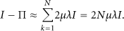
We further assume that μ is small enough so that ${\bar{F}}_k$ can be approximated as

$\begin{array}{c}{\bar{F}}_k\approx I-2\mu \lambda I.\end{array}$

(41)

So, ${\bar{F}}_k$ is now a diagonal matrix and as a result, matrix ${\Pi }_{k,\ell }=\Pi ={\bar{F}}_1{\bar{F}}_2\cdots {\bar{F}}_N$ will be diagonal as well. For small μ, we have $(1-2\mu \lambda {)}^N\approx (1-2\mu N\lambda )$ , then Π can be approximated as

$\begin{array}{cc}\hfill \Pi & =\left(I-2\mu \lambda I\right)\left(I-2\mu \lambda I\right)\cdots \left(I-2\mu \lambda I\right)\hfill \\ \hfill & \approx \left(1-2\mu N\lambda \right)I,\hfill \end{array}$

(42)

so that

$\begin{array}{c}I-\Pi \approx {\displaystyle \sum }_{k=1}^{N}2\mu \lambda I=2N\mu \lambda I.\end{array}$

(43)

Similarly, using the assumptions in (A.6), we have

$\begin{array}{c}{g}_k={\mu }^2{\sigma }_{v,k}^2\lambda r^T+{\sigma }_{c,k}^2\left(1-2\mu \lambda \right)r^T,\end{array}$

(44)

so that $a_k$ becomes

$\begin{array}{c}{a}_k\approx {\displaystyle \sum }_{k=1}^N{g}_k=\left({\displaystyle \sum }_{k=1}^N\left({\mu }^2{\sigma }_{v,k}^2\lambda +{\sigma }_{c,k}^2\left(1-2\mu \lambda \right)\right)\right)r^T.\end{array}$

(45)

Now, replacing (43) and (45) into (35) and using $r^{T}r=M$ , we obtain

$\begin{array}{c}{\eta }_k=\frac{M}{2\mu \lambda N}{\displaystyle \sum }_{k=1}^N\left({\mu }^2{\sigma }_{v,k}^2\lambda +{\sigma }_{c,k}^2(1-2\mu \lambda )\right),\end{array}$

(46)

similarly, we can find the following approximations for EMSE and MSE as

$\begin{array}{c}{\zeta }_k=\frac{M}{2\mu N}{\displaystyle \sum }_{k=1}^N\left({\mu }^2{\sigma }_{v,k}^2\lambda +{\sigma }_{c,k}^2\left(1-2\mu \lambda \right)\right),\\ {\xi }_k={\zeta }_k+{\sigma }_{v,k}^2.\end{array}$

(47)

We can easily conclude from (46)-(47) that the MSD, EMSE, and MSE curves are not monotonically increasing function of step size parameter. In Figure 2, we have shown the MSD as a function of μ when $N=20$ , $M=5$ , $\lambda =1$ , ${\sigma }_v^2=0.02$ and for different values of ${\sigma }_c^2$ . As it is clear from Figure 2, for ${\sigma }_c^2=0$ (i.e., noiseless links), the MSD curve is a monotonically increasing function of μ.

Figure 2

The steady-state MSD (in dB) curve as a function of μ and for different values of ${\sigma }_c^2$ .

Remark 1.

To explain this behavior, we consider again the update (6). For small μ, the channel noise term say $q_{k,i}$ is dominant term in update equation, so as $\mu \to 0$ the steady-state performance deteriorates. As μ increases, the effect of channel noise term decreases, and finally as μ becomes larger, the steady-state performance deteriorates again like any adaptive algorithm.

Remark 2.

The optimal step size for MSD is given by

$\begin{array}{c}{\mu }_o=\sqrt{\frac{{\sum }_{k=1}^N{\sigma }_{c,k}^2}{{\sum }_{k=1}^N\lambda {\sigma }_{v,k}^2}}.\end{array}$

(48)

It must be noted that (48) is also the optimal step size for EMSE and MSE curves.

Remark 3.

Note that according to the given results in [10], as step size becomes smaller $(\mu \to 0)$ , steady-state values of MSD, EMSE, and MSE in each node should be more smaller too, but this is not the case in the presence of noisy links. In fact, μ must be chosen more carefully in real world.

5. Simulation

In this section, we provide computer simulations to compare the theoretical expressions with simulation results. To conduct our simulation results, we consider the following steps:

• (1)

consider a network with noisy link and generate the measurement and regression data,

(2)

select a parameter $w^o$ (which is known for us but unknown for DILMS algorithm),

(3)

let the DILMS algorithm estimate $w^o$ in WSN with noisy links and data (generated in step 1),

(4)

obtain the MSD, EMSE, and MSE simulation results,

(5)

we apply the data (generated in step 1) to our derived theoretical results,

(6)

finally, we compare the resultant simulation results with derived theoretical results.

To this aim, we consider a distributed network with $N=20$ nodes, and choose $M=4$ and $w^o=[1\hspace{0.5em}1\hspace{0.5em}\cdots \hspace{0.5em}1{]}^T/\sqrt{M}$ .

5.1. Regressors with Shift Structure

Although the analysis relied on the independence assumptions, simulations presented in this subsection were carried out using regressors with shift structure to cope with realistic scenarios. The regressors are generated at each node k according to the following recursion:

$\begin{array}{c}{u}_k\left(i\right)={\alpha }_k{u}_k\left(i-1\right)+{\beta }_k{\tau }_k\left(i\right).\end{array}$

(49)

The expression above describes a first-order autoregressive (AR) process with a pole at ${\alpha }_k$ , ${\tau }_k$ is a white, zero-mean, Gaussian random sequence with unity variance or a uniform random sequence with unity variance, ${\alpha }_k\in (\mathrm{0,0.5}]$ and ${\beta }_k=\sqrt{{\sigma }_{u,k}^2(1-{\alpha }_k^2)}$ . In this way, the covariance matrix $R_{u,k}$ of the regressors $u_{k,i}$ is $M\times M$ Toeplitz matrix with entries $r_k(m)={\sigma }_{u,k}^2{\alpha }_k^{|m|}$ , $m=\mathrm{0,1},2,\dots ,M-1$ with ${\sigma }_{u,k}^2\in [\mathrm{0,0.5})$ . The MSD, EMSE, and MSE are obtained by averaging the last 200 samples. Each curve is obtained by averaging over 100 independent experiments. The steady-state curves are generated by running the network learning process for 2000 iterations. We consider real data ( $\gamma =2$ ).

We assume that for node k, covariance matrix $Q_k$ is a diagonal matrix and has different values at the diagonal so

$\begin{array}{c}{Q}_k={\left[\begin{array}{cccc}{\delta }_{k,1}& 0& \cdots & 0\\ 0& {\delta }_{k,2}& \cdots & 0\\ ⋮& ⋮& \ddots & ⋮\\ 0& 0& \cdots & {\delta }_{k,M}\end{array}\right]}_{M\times M}.\end{array}$

(50)

In fact, at each node k, the noise term $q_{k,i}$ is generated to result the required (assumed) covariance matrix $Q_k$ . The statistical profiles for the mentioned parameters are illustrated in Figure 3.

Figure 3

Node profile and channel noise information.

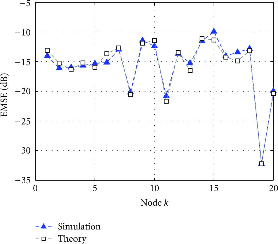
In Figures 4–6, the steady-state of MSD, EMSE, and MSE for $\mu =0.03$ are plotted, respectively. It is clear from Figures 4–6 that there is a good match between simulation and theory. Note also that despite the diverse statistical profile, the MSD in Figure 4 is roughly even over the network. On the other hand, the EMSE and the MSE are more sensitive to local statistics, as depicted in Figures 5 and 6.

Figure 4

Steady-state MSD versus node, $\mu =0.03$ .

Figure 5

Steady-state EMSE versus node, $\mu =0.03$ .

Figure 6

Steady-state MSE versus node, $\mu =0.03$ .

In Figures 7 and 8, the MSD and EMSE for different values of μ for node $k=10$ are plotted. We note that unlike the ideal link case [10], here, the steady-state MSD and EMSE (and also MSE) are not a monotonically increasing function of μ.

Figure 7

Steady-state MSD versus μ, node $k=10$ .

Figure 8

Steady-state EMSE versus μ, node $k=10$ .

5.2. Independent Regressors

In this case, we assume that the regressors data arise from independent Gaussian, where their eigenvalue spread is $\rho =5$ . We assume $Q_k=10^{-3}{I}_M$ for channel noise. The observation noise variance ${\sigma }_{v,k}^2$ and $\mathrm{Tr}\hspace{0.17em}[R_{u,k}]$ are shown in Figure 9. In Figures 10 and 11, the steady-state of MSD and EMSE for $\mu =0.001$ are plotted. It is clear from Figures 10 and 11 that there is a good match between simulation and theory.

Figure 9

The Observation noise power profile, (a) ${\sigma }_{v,k}^2$ and (b) $\mathrm{Tr}\hspace{0.17em}[R_{u,k}]$ .

Figure 10

Steady-state MSD versus node, $\mu =0.001$ .

Figure 11

Steady-state EMSE versus node, $\mu =0.001$ .

6. Conclusions and Future Work

In this paper, we derived theoretical relations to predict the performance of incremental distributed least-mean square algorithm (DILMS) when the links between nodes were noisy. Starting with the weighted energy conservation relation, we derived a variance relation for our problem. However, The important result is that unlike the ideal link case, the steady-state MSD, EMSE, and MSE are not a monotonically increasing function of step size when links are noisy. The simulation results revealed that there is good match between the derived closed-form expressions for MSD, EMSE, and MSE for every node in the network and the simulation results. Note that although in this paper we focused on the LMS adaptive filter, we can extend it for other adaptive filters. In our future work, we will consider more sophisticated cooperation modes (rather than incremental mode), such as diffusion mode.