Sage Journals: Discover world-class research

Abstract

This paper investigates the locomotion of a walking robot by delivering a comparative study of three different biologically inspired walking gaits, namely: tripod, ripple, and wave, in terms of ground slippage they experience while walking. The objective of this study is to identify the gait model which experiences the minimum slippage while walking on a ground with a specific coefficient of friction. To accomplish this feat, the robot is steered over a reference path using a waypoint navigation algorithm, and the divergence of the robot from the reference path is investigated in terms of slip errors. Experiments are conducted through closed-loop simulations using an open dynamics engine which emphasizes the fact that due to uneven and unsymmetrical distribution of payload in tripod and ripple gait models, the robot experiences comparatively larger drift in these gaits than when using the wave gait model in which the distribution of payload is even and symmetrical on both sides of the robot body. The paper investigates this phenomenon on the basis of force distribution of supporting legs in each gait model.

1. Introduction

The development of a scheme to generate leg sequential movements representing particular walking gaits is an important aspect in the design and realization of walking systems [1].

In order to realize the utilization and implementation of walking robots in real world scenarios and natural environments, generation of appropriate walking gaits is an imperative requirement. The performance of a walking gait is generally ensured in terms of its mobility and stability as addressed in [2].

Gait analysis involves inspection and evaluation of various gait variables that include its speed, stability, adaptability to a specific terrain, and so forth. Periodic gaits which include tripod, wave and in-phase gaits as discussed in [3, 4] investigate the walking patterns in terms of coordinated placements of footholds and body motions in order to transit from one pose to another. Furthermore, in the context of generation of stepping patterns for walking, free gaits have been studied in [5]. Follow-the-leader gaits as discussed in [6, 7] deliver a study on adaptive gaits. In another related study [8], stepping sequences of insects are investigated to describe a straight-line walking gait for a hexapod robot by considering alternating tripod gaits.

The purpose of this paper is to deliver a comparative study on various walking gaits found in nature. The study encompasses the comparison of walking gaits in terms of their speed and ground slippage while walking in a dynamic environment. During walking, the leg-ground interactions result in reaction forces at the contact points. These reaction forces can be approximated by applying impact with friction theory as reported in [9]. In order to evaluate the slippage experienced by the robot while walking with a specific gait, slip errors are investigated herein terms of robot's divergence from its reference path and coefficients of friction.

A waypoint navigation algorithm is further proposed based on sensor-based attitude guidance. The proposed algorithm is used to steer the robot through a series of reference waypoints, and the divergence of the robot from the reference path is analyzed in terms of tracking errors (heading and displacement).

The first part of the paper deals with the modeling of the robot in terms of its kinematic equations and computer-aided design. The kinematic equations are formulated using the forward and inverse kinematics of serial manipulators. The work done in [10] has been reviewed in this context to understand the kinematic model of our robot leg that is inspired from the leg structure of a stick insect. A stick insect leg consists of four functional segments: the coxa (c), the femur (f, which is fused to a very short segment, the trochanter), the tibia (t), and the foot (ft, or tarsus) as reported in [10]. In order to simplify the kinematic configuration of a robotic leg inspired from the leg structure of a stick insect, the joint of the foot and the foot itself are neglected. Therefore, a stick insect leg can be modelled as a serial manipulator with three revolute joints, resulting in a 3-DOF serial manipulator as investigated in [10].

The second part of the paper describes a waypoint navigation algorithm to steer the robot through a series of desired way-points. Simulations are carried out in an open dynamic simulation environment using a software physics engine “AGEIA PhysX” provided by Microsoft Robotics Developer Studio. Microsoft Robotics Developer Studio provides a visual simulation environment that is a 3D simulator with full physics simulation and can be used to prototype new algorithms or robots [11].

2. Modeling and Design

The robot reported here is a hexapod robot which consists of six-legs attached around its central body in a symmetrical and biological manner. In literature, various studies [12–16] describe the designs and architectures of robotic platforms inspired from legged creatures found in nature.

The design of our robot's leg resembles a serial manipulator with three degrees of freedom. Figure 1 shows the CAD model of the robot designed in Pro-Engineer. The legs are numbered from 1 to 6. Legs 1, 2, and 3 correspond to the right side of the robot body while the left side legs are numbered as 4, 5, and 6.

Figure 1:

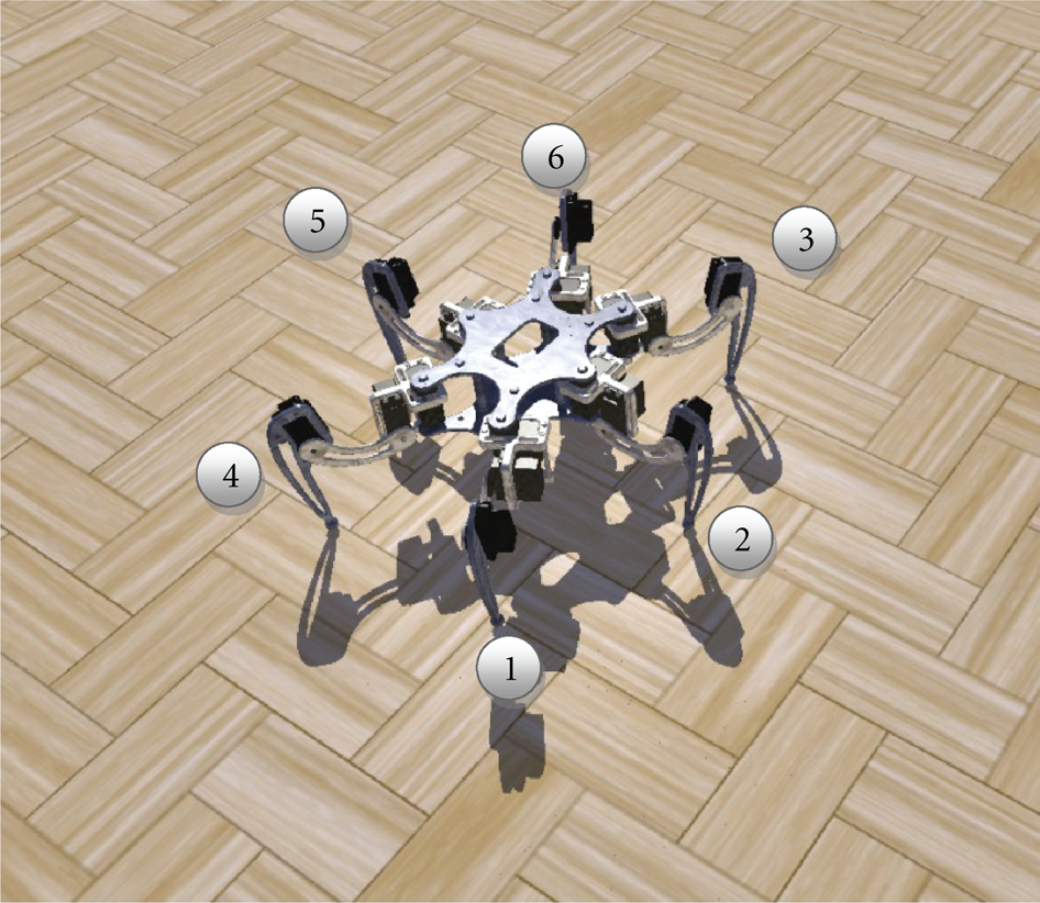
Physical model of the robot.

2.1. Actuator Model

The leg of the robot consists of three links, coxa, femur, and tibia represented by their lengths l_c, l_f, and l_t, respectively, interconnected through revolute joints. From the body towards the foot, the joints are called body-coxa joint (θ_c), coxa-femur joint (θ_f), and femur-tibia joint (θ_t).

The kinematic configuration resembles an insect-like (stick insect) configuration that is, the axis of rotation of the joint θ_f lies parallel to the axis of rotation of the joint θ_t and perpendicular to the axis of rotation of the joint θ_c. Thus, there are two motion axes in a common plane that is perpendicular to the plane containing the third motion axis. Figure 2 shows this kinematic configuration of the leg in terms of its links and their motion axes.

Figure 2:

Configuration of the leg of the robot.

2.2. Kinematic Modeling

The work done in this paper is an extension of the work presented in [17]. The kinematic model of the robot has already been discussed in [17] in great detail, therefore, the kinematic equations derived in [17] are reformulated here to describe the underlying kinematic model for our proposed motion algorithm. The position of the foothold with respect to robot's body frame of reference is computed using forward kinematics and is described in (1).

\begin{gathered} {X_{foot}}_{i}^{B} = \cos θ_{c} (l_{c} + l_{t} \cos θ_{f + t} + l_{f} \cos θ_{f}), \\ {Z_{foot}}_{i}^{B} = \sin θ_{c} (l_{c} + l_{t} \cos θ_{f + t} + l_{f} \cos θ_{f}), \\ {Y_{foot}}_{i}^{B} = - l_{t} \sin θ_{f + t} - l_{f} \sin θ_{f} . \end{gathered}

(1)

The angular motion of the robot's body is described in terms of its rotation angles, roll (φ), pitch (ψ), and yaw (γ) around the z-axis, x-axis, and y-axis, respectively. The transformation from the robot's body frame to the global frame is defined by (2) represented as a general homogeneous transformation expression.

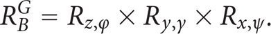
\begin{matrix} R_{B}^{G} & = R_{z, φ} \times R_{y, γ} \times R_{x, ψ} \end{matrix} .

(2)

Therefore, the transformation from foothold to the global frame for an individual leg can be written as described in (3).

\begin{matrix} [\begin{bmatrix} {P_{x}}_{i}^{G} \\ {P_{y}}_{i}^{G} \\ {P_{z}}_{i}^{G} \end{bmatrix}] & = R_{B}^{G} \times [\begin{bmatrix} {X_{foot}}_{i}^{B} \\ {Y_{foot}}_{i}^{B} \\ {Z_{foot}}_{i}^{B} \end{bmatrix}] \end{matrix} .

(3)

Solving (3) computes foothold positions in global frame of reference as expressed in (4).

\begin{matrix} {P_{x}}_{i}^{G} & = \cos γ \cos φ {X_{foot}}_{i}^{B} - \cos γ \sin φ {Y_{foot}}_{i}^{B} + \sin γ {Z_{foot}}_{i}^{B}, \\ {P_{y}}_{i}^{G} & = (\cos ψ \sin φ + \sin ψ \sin γ \cos φ) {X_{foot}}_{i}^{B} \\ + (\cos ψ \cos φ - \sin ψ \sin γ \sin φ) {Y_{foot}}_{i}^{B} \\ - \sin ψ \cos γ {Z_{foot}}_{i}^{B}, \\ {P_{z}}_{i}^{G} & = (\sin ψ \sin φ - \cos ψ \sin γ \cos φ) {X_{foot}}_{i}^{B} \\ + (\sin ψ \cos φ + \cos ψ \sin γ \sin φ) {Y_{foot}}_{i}^{B} \\ + \cos ψ \cos γ {Z_{foot}}_{i}^{B} . \end{matrix}

(4)

Equation (4) describes the forward or direct kinematics solution to represent the position of a foothold in three dimensional spaces in global frame of reference, while the joint angles are computed using the inverse kinematic model and are described by (5) as reported in [17].

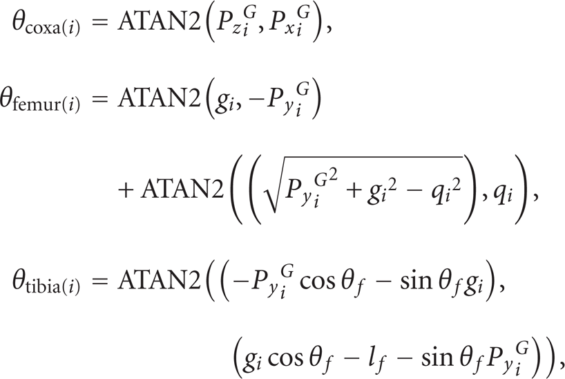
\begin{matrix} θ_{coxa (i)} & = ATAN2 ({P_{z}}_{i}^{G}, {P_{x}}_{i}^{G}), \\ θ_{femur (i)} & = ATAN2 (g_{i}, - {P_{y}}_{i}^{G}) \\ + ATAN2 ((\sqrt{{P_{y}}_{i}^{G}^{2} + {g_{i}}^{2} - {q_{i}}^{2}}), q_{i}), \\ θ_{tibia (i)} & = ATAN2 ((- {P_{y}}_{i}^{G} \cos θ_{f} - \sin θ_{f} g_{i}), \\ (g_{i} \cos θ_{f} - l_{f} - \sin θ_{f} {P_{y}}_{i}^{G})), \end{matrix}

(5)

where, g_i = (P_x_i^Gcos θ_c − l_c+P_z_i^Gsin θ_c) and $q_{i} = ({g_{i}}^{2} + {l_{f}}^{2} + {P_{y}}_{i}^{G}^{2} - {l_{t}}^{2}) / 2 l_{f}$ .

3. Waypoint Navigation

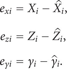
The overall control framework as shown in Figure 4 encompasses several subsystems sharing information with each other. The algorithm starts with the computation of position and orientation vectors which describe the location (X_i,Z_i,γ_i) of a desired waypoint in terms of a finite number of sections, where each section represents a Δ change in x-axis (ΔX_i) & z-axis (ΔZ_i), and a Δ change about y-axis (Δγ_i) in global frame of reference, as further illustrated in (6) and pictorially demonstrated in Figure 3.

{\begin{cases} [\begin{bmatrix} X_{i + 1} \\ Z_{i + 1} \\ γ_{i + 1} \end{bmatrix}] = [\begin{bmatrix} X_{i} \\ Z_{i} \\ γ_{i} \end{bmatrix}] + [\begin{bmatrix} {∆ X}_{i} \\ {∆ Z}_{i} \\ ∆ γ_{i} \end{bmatrix}] \\ [\begin{bmatrix} {∆ X}_{i} \\ {∆ Z}_{i} \\ ∆ γ_{i} \end{bmatrix}] = [\begin{bmatrix} \sum_{j = 1}^{m} {δ x}_{j} \\ \sum_{j = 1}^{m} {δ z}_{j} \\ \sum_{j = 1}^{m} {δ γ}_{j} \end{bmatrix}] \\ δ \leq length of leg stroke \\ m = number of finite sections. \end{cases}

(6)

Figure 3:

Motion planning of the robot using waypoint navigation.

Figure 4:

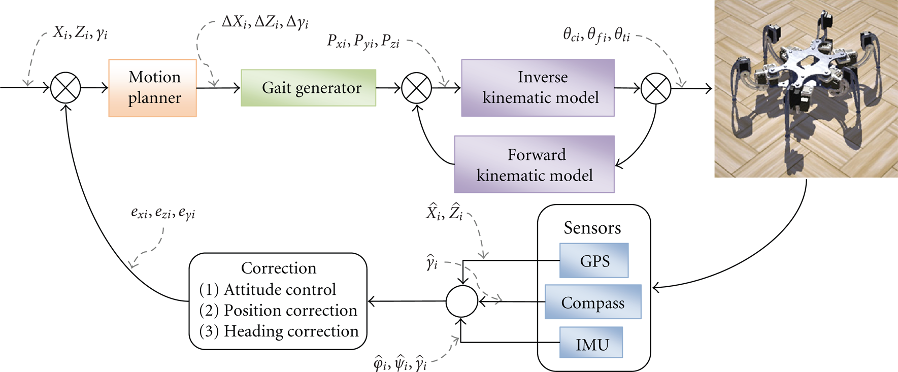
Overall framework of the robot control.

The control loop uses the previously described inverse kinematic model to compute the desired joint angles for legs L_i for a desired foothold location that is described in terms of its position and orientation in global frame of reference. The computed joint angles (θ_{c
i},θ_{f
i},θ_{t
i}) are converted into their respective PWM signals which are sent over to the servos using a servo sequential control hardware resulting in a new position (X_i+1,Z_i+1,γ_i+1) of the robot.

The heading γ_i+1 for every next waypoint is computed using (7).

γ_{i + 1} (t) = ATAN2 (\frac{Z_{i + 1} (t) - Z_{i} (t)}{X_{i + 1} (t) - X_{i} (t)}) .

(7)

Thus, the motion planner computes the position and orientation vectors for a desired waypoint and invokes the gait generator. The Gait generator computes the foothold positions using (4) to construct a cyclic gait. At each iteration step, the sensors data is used as control feedback in the control loop. The feedback from GPS sensor is used to track and correct the absolute position, whereas the feedback from the compass sensor is used to track and correct the absolute heading of the robot in global frame of reference, further explained in (8).

\begin{matrix} e_{x i} & = X_{i} - {\hat{X}}_{i}, \\ e_{z i} & = Z_{i} - {\hat{Z}}_{i}, \\ e_{γ i} & = γ_{i} - {\hat{γ}}_{i} . \end{matrix}

(8)

These tracking corrections (position & heading) are computed by the correction block shown in Figure 4 which also acts as an independent attitude controller responsible for keeping the body of the robot leveled above the groundthroughout its locomotion. The rotation angles are measured about the motion centroid of the robot using IMU feedback.

In summary, the motion planner plans the path of the robot through the reference waypoints, the gait generator generates foothold positions based on sequential pattern generation and the kinematic engine computes the required joint angles based on foothold positions to traverse the robot to its next position at every ith step. The onboard sensors provide data in terms of absolute position and attitude of the robot that is used as control feedback to compute the drift corrections.

The gait generator generates stepping patterns through sequential cycling of swing, drop, and stance phases. The swing phase describes a transition in which a leg lifts vertically upward and traverses to acquire the next planned foothold position (P_x_i+1^G,P_z_i+1^G) in air, further described in (9). The swing phase is followed by the drop phase in which the lifted leg is landed until it rests on ground

Swing = function (Lift, Stroke),

(9)

where Lift : Transition from P_y_i^G to P_y_i+1^G, Stroke : Transition from P_x_i^G to P_x_i+1^G and P_z_i^G to P_z_i+1^G.

The stance phase describes a transition in which the involved legs support and advance the body of the robot by an amount described in (10).

Body Motion = \frac{Stroke}{number of steps in the gait cycle} .

(10)

4. Simulations

The proposed algorithm is tested here by simulating the robot using tripod, ripple, and wave gait models using a constant gait speed of 5 cm/sec which is chosen to be adequate enough to evaluate the locomotion on flat surfaces for a robot of this size. In particular, each phase (swing, drop, and stance) in the gait cycle executes at a constant speed of 5 cm/sec. The prime objective is to investigate the locomotion of the robot using different gait models in the presence of external disturbances. Since, each gait is unique in terms of its planned footholds and stepping pattern with unique number of steps per cycle, the behavior of the robot's locomotion in the presence of external disturbances (ground slippage) can be inspected and evaluated.

In the context of dealing with friction in walking machines, numerous studies [18–20] have employed the general coulomb friction model to generate stepping patterns based on the ground reaction forces. In a related study [18], an excellent approach of pattern generation based on preview control theory is implemented on a biped robot to perform desired motions on a low friction floor.

Thus, in the light of these research studies, the slip that the robot may experience while walking is evaluated here by considering the coefficients of friction and the general coulomb friction model. The tangential friction force f_t is equal to the product of vertical normal force f_y and coefficient of ground friction μ_ground as reported in [18, 19].

f_{t} = μ_{ground} f_{y} .

(11)

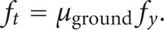
Thus, when the foot is not slipping, we can rewrite the above equation as follows:

f_{t} \leq μ_{ground} f_{y} .

(12)

Here, we define a combined coefficient of effective friction that is computed online using the forces involved at the contact points during the impact (leg-ground interaction), further described in (13).

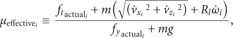
\begin{matrix} μ_{{effective}_{i}} \equiv \frac{{f_{t}}_{{actual}_{i}} + m (\sqrt{({\dot{v}}_{x_{i}}^{2} + {\dot{v}}_{z_{i}}^{2})} + R_{l} {\dot{ω}}_{i})}{{f_{y}}_{{actual}_{i}} + m g}, \end{matrix}

(13)

where μ_effective indicates the minimum friction coefficient to represent a behavior for stable walking without slip or drift, ${\dot{v}}_{x_{i}}^{2}$ & ${\dot{v}}_{z_{i}}^{2}$ and ${\dot{ω}}_{i}$ are the linear and angular components of slip acceleration approximated using rate sensors, R_l is the transformation matrix of the involved leg “L_i”, g is the gravitational acceleration and f_t_actual & f_y_actual are the tangential and normal forces estimated online using force sensing resistors. Hence, we can formulate the behaviour for stable walking using a nonslip condition as described in (14).

μ_{effective} \leq μ_{ground} .

(14)

Thus, μ_effective is computed online considering the actual ground reaction forces involved during the impact phase coupled with the lateral and longitudinal components of the slip forces approximated using slip accelerations atthe contact points. Furthermore, μ_effective is used in this paper as a performance measure to evaluate the mobility and stability of different hexapod walking gaits (inspired from stepping patterns of legged creatures found in nature) on a surface with known coefficients of ground friction to conduct a comparative analysis.

It is considered in this paper that, if the inequality presented in (14) is satisfied for a given walking pattern, we can conclude that the robot will walk without significant divergence from the reference path in the presence of slip as an external disturbance. In the light of these ideas, a simulation is set-up using Microsoft Robotics Studio Visual Simulation Environment constituting a flat ground having 0.45 as the coefficient of ground friction. The simulations are performed with tripod, ripple and wave gait models and the locomotion of the robot is evaluated in terms of μ_effective computed online considering the simulation results.

4.1. Simulation Test 1—Tripod Gait

Tripod gait is the typical gait of a six-legged robot to realize walking with high mobility. Its core methodology is to divide the six legs into two groups. One's function is to support the body and promote the forward traversing of the robot while the other group's function is to swing for the preparation for the next stance as discussed in [21, 22]. Thus, the alternative cycling of the stance phase and the swing phase constitutes the kinematic procession of the robot in the tripod gait.

4.1.1. Group 1: Legs 1, 5, and 3, Group 2: Legs 2, 4, and 6

Step 1. Group 1 swings and Group 2 propels the body.

Step 2. Group 1 down and Group 2 propels the body.

Step 3. Group 2 swings and Group 1 propels the body.

Step 4. Group 2 down and Group 1 propels the body.

The tripod gait modeled in this paper is a 4-step cyclic gait as illustrated in Figure 5.

Figure 5:

Pictorial representation of tripod gait 4-step cycle.

In test 1, the robot is traversed with the proposed tripod gait model, and the path traced by the robot is shown in Figure 14 by the blue colored plot. The tracking errors are shown in Figure 6 in terms of displacement and heading errors.

Figure 6:

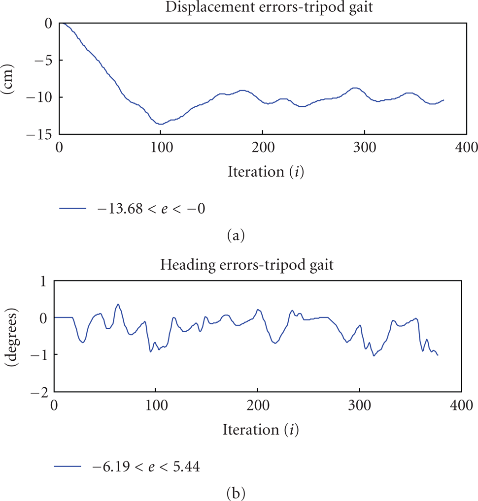
Tripod gait—tracking errors, average speed 0.29 m/sec.

The tracking errors plot describes a maximum drift of 13 cm off the desired course and a heading error of ±5.5 degrees approximately. With a short gait cycle and grouping of alternate legs, the robot completed the path in 58 seconds; however, due to large inertial forces arising from quick body propulsions in the tripod gait, the no-slip inequality condition is violated for a number of times during the locomotion of the robot as illustrated in Figure 7.

Figure 7:

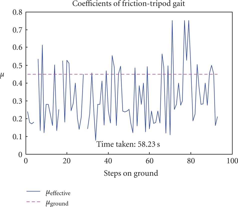
Tripod gait—coefficients of friction plot.

4.2. Simulation Test 2—Ripple Gait

The ripple gait model investigated in this paper constitutes the following leg stepping pattern.

Step 1. Leg 1 down, Leg 5 swing, Legs (2, 3, 4, 6) propel the body.

Step 2. Leg 5 down, Leg 3 swing, Legs (1, 2, 4, 6) propel the body.

Step 3. Leg 3 down, Leg 4 swing, Legs (1, 2, 5, 6) propel the body.

Step 4. Leg 4 down, Leg 2 swing, Legs (1, 3, 5, 6) propel the body.

Step 5. Leg 2 Down, Leg 6 Swing, Legs (1, 3, 4, 5) propel the body.

Step 6. Leg 6 down, Leg 1 swing, Legs (2, 3, 4, 5) propel the body.

Thus, in ripple gait model, there are always two alternate legs in the swing phase whereas the remaining four legs support and propel the body in the direction of the motion. In test 2, the robot is traversed with the aforesaid ripple gait model, and the path traced by the robot is shown in Figure 14 by the red colored plot. The tracking errors are shown in Figure 8. Due to uneven weight distribution on both sides of the robot body and short gait cycle, the no-slip inequality is still violated for a number of times as shown in Figure 9.

Figure 8:

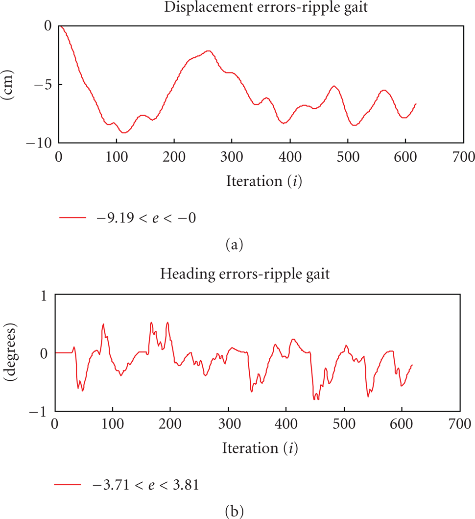
Ripple gait—tracking errors, average speed 0.15 m/sec.

Figure 9:

Ripple gait—coefficients of friction plot.

4.3. Simulation Test 3—Wave Gait

The wave gait model investigated in this paper constitutes the following leg stepping pattern.

Step 1. Leg 1 swings.

Step 2. Leg 1 down and all legs propel the body.

Step 3. Leg 2 swings.

Step 4. Leg 2 down and all legs propel the body.

Step 5. Leg 3 swings.

Step 6. Leg 3 down and all legs propel the body.

Step 7. Leg 4 swings.

Step 8. Leg 4 down and all legs propel the body.

Step 9. Leg 5 swings.

Step 10. Leg 5 down and all legs propel the body.

Step 11. Leg 6 swings.

Step 12. Leg 6 down and all legs propel the body.

Thus, in the wave gait model, legs sequentially go into the swing phase one after the other in a wave-like fashion, while the remaining five legs support the body giving more kinematic stability to the locomotion cycle. Furthermore, the body is propelled by all the six legs resulting in a precise body displacement due to even distribution of weight on the supporting legs on both sides of the robot body. In test 3, the robot is traversed with the proposed wave gait model, and the path traced by the robot is shown in Figure 14 by the black colored plot. The tracking errors are shown in Figure 10.

Figure 10:

Wave gait—tracking errors, average speed 0.052 m/sec.

The motion of the robot in the visual simulation environment provided by Microsoft Robotics Developer Studio is shown in Figures 12 and 13.

For a comparative representation, the paths traced by the robot when steered using the proposed tripod, ripple and wave gait models are shown in Figure 14. The black circles represent the desired waypoints while the blue, red, and black colored plots represent the paths traced by the robot.

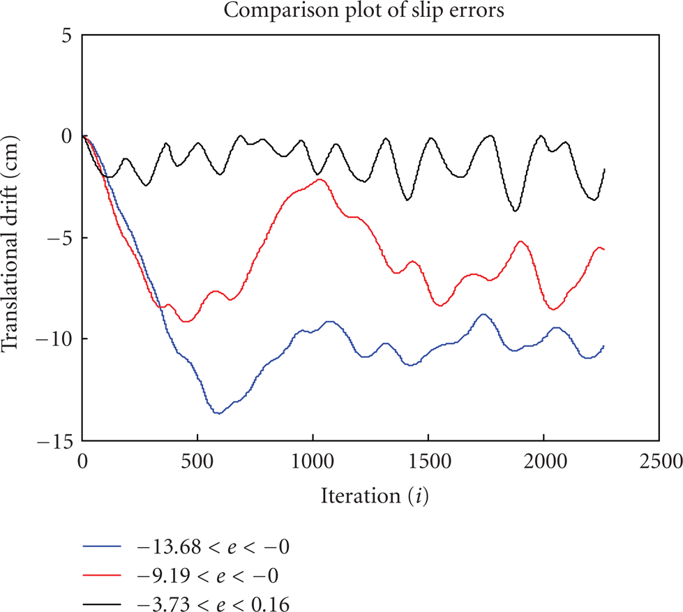
Figures 15 and 16 present a comparative representation of translational and rotational slip errors for the three simulation tests.

5. Discussions and Conclusion

This paper investigates the locomotion of a hexapod robot by proposing three different gait models for walking. The leg sequencing patterns are taken from biologically inspired walking gaits which include tripod, ripple, and wave.

The tripod gait as discussed in Section 4.1 is a 4-step cyclic gait in which three legs at a time go into the swing phase while, the remaining three legs support the body. The support distribution of the legs is unsymmetrical on both sides of the body since on one side there is one leg in the stance phase while on the other side there are two legs. Thus, the force distribution is unsymmetrical. Since the body of the robot is propelled during the swing phase, the unsymmetrical weight distribution results in irregular force distribution.

This unsymmetrical force distribution phenomenon affects the ripple gait model as well. As illustrated by the gait pattern in Section 4.2, there are always two legs which go into the swing phase simultaneously. Thus, the active payload is supported by the remaining 4 legs. Since the body is propelled during the swing phase therefore, the unsymmetrical weight distribution results in irregular force distribution.

As a result, the motion is wavy, and tracking errors are significant in both the cases when using the tripod and ripple gait models as shown in Figures 15 and 16. Furthermore, a comparative study of Figures 7 and 9 yields that when using the tripod or ripple gait models, there are steps on the ground where the combined coefficient of effective friction gets larger than the ground friction coefficient which violates the no-slip condition defined in (14).

In the wave gait model as discussed in Section 4.3, only one leg goes into swing phase at a time, and thus the body of the robot is supported by the remaining 5 legs. This in one place increases the static stability of the robot. In the second place, the body of the robot is propelled only when all the legs are on the ground, that is, supporting the body. Since the support distribution is symmetrical on both sides of the body, the force distribution is also even and regular on both the sides. Figure 11 shows that during the whole course, the no-slip condition is least violated, and the tracking errors as portrayed by Figure 10 are thus the minimum.

Figure 11:

Wave gait—coefficients of friction plot.

Figure 12:

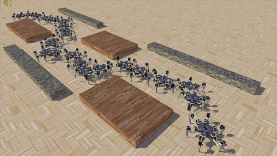
Visual representation of the robot driven on the desired path.

Figure 13:

Top view of the simulation environment.

Figure 14:

Paths traced by the robot with tripod, ripple and wave gait types.

Figure 15:

Tracking errors in terms of displacements errors.

Figure 16:

Tracking errors in terms of headings errors.

To conclude, wave gait model as described in this paper offers even and symmetrical weight distribution during the stance phase resulting in better kinematic stability in terms of translational and rotation drift in comparison to the tripod and ripple gait models. The displacement errors have improved from 13 cm in tripod gait and 9 cm in ripple gait to 3.7 cm in wave gait approximately. Similarly, the heading errors have improved from 6° in tripod gait and 3.7° in ripple gait to 1.6° in wave gait approximately.

Thus, the work done in this paper has helped in realizing the effect of different walking patterns on the locomotion of the robot in path following tasks through ground-foot interactions. By keeping the gait speed fixed, the simulation results have emphasized the fact that due to uneven weight distribution in tripod and ripple gait models, the robot experiences comparatively larger drift in these gaits than when using the wave gait model in which weight distribution is even and symmetrical on both sides of the robot body. This fact has also been accentuated through the plots of coefficients of friction as shown in Figures 7, 9, and 11. A comparative evaluation of these figures shows that the no-slip inequality as described by (14) is least violated when using the wave gait model. As a result, the locomotion of the robot is found kinematically more stable, and the slip errors are found minimal in the wave gait model than when using the ripple and tripod gait models.

The paper has evaluated this phenomenon by investigating the force distribution of supporting legs in three different cyclic gait models.

References

Anthon Lewis

Fagg

A. H.

, and Bekey

G. A.

, “Genetic algorithms for gait synthesis in a hexapod robot,” in Recent Trends in Mobile Robots, Zheng

Y. F.

, Ed., pp. 317–331, World Scientific, New Jersey, NJ, USA, 1994.

Hiroshi

and Masayoshi

, “Adaptive gait for a quadruped robot on 3D path planning,” in Proceeding of the IEEE International Conference on Robotics & Automation, pp. 2049–2054, Taipei, Taiwan, September 2003.

Rabbo

, “Gait analysis and shaft synchronization of hexapod walking vehicle via fuzzy logic,” in Proceeding of the 7th International Multi-Conference on Systems, Signals and Devices, (SSD ′10), June 2010.

Lee

W. J.

and Orin

D. E.

, “Omni-directional control of a multi-legged robot vehicle using periodic gaits,” in Proceedings of the ASME International Computers in Engineering Conference, 1985.

McGhee

and Iswandhi

G. I.

, “Adaptive locomotion of a multi-legged robot over rough terrain,” IEEE Transactions on Systems, Man, and Cybernetics, vol. SMC-9, pp. 176–182, 1979.

Ozguner

Tsai

, and McGhee

, “An approach to the use of terrain preview information in rough-terrain locomotion by a hexapod walking machine,” The International Journal of Robotics Research, vol. 3, no. 2, pp. 134–146, 1984.

Shih

and Klein

C. A.

, “Adaptive gait for legged walking machines over rough terrain,” IEEE Transactions on Systems, Man and Cybernetics, vol. 23, no. 4, pp. 1150–1155, 1993.

Jianhua

, “Design and kinematic simulation for Six-DOF leg mechanism of hexapod robot,” in Proceeding of the IEEE International Conference on Robotics and Biomimetics, (ROBIO ′06), pp. 625–629, Kunming, China, December 2006.

Pfeiffer

and Glocker

, Multi-Body Dynamics with Unilateral Contacts, John Wiley & Sons, New York, NY, USA, 1996.

10.

Durr

Schmitz

, and Cruse

, “Behaviour-based modelling of hexapod locomotion: linking biology and technical application,” Arthropod Structure & Development, vol. 33, no. 3, pp. 237–250, 2004.

11.

Johns

and Taylor

, Professional Microsoft Robotics Developer Studio, Wiley, Indianapolis, Ind, USA, 2008.

12.

Delcomyn

and Nelson

M. E.

, “Architectures for a biomimetic hexapod robot,” Robotics and Autonomous Systems, vol. 30, no. 1, pp. 5–15, 2000.

13.

Quinn

R. D.

Nelson

G. M.

Bachmann

R. J.

Kingsley

D. A.

Offi

, and Ritzmann

R. E.

, “Insect designs for improved robot mobility,” in Proceedings of the 4th International Conference on Climbing and Walking Robots, pp. 69–76, Berns and Dillmanneds, 2001.

14.

Altendorfer

Moore

Komsuoglu

, “RHex: a biologically inspired hexapod runner,” Autonomous Robots, vol. 11, no. 3, pp. 207–213, 2001.

15.

Klaassen

Kirchner

, and Spenneberg

, “A biologically inspired approach towards robust real world locomotion in an eight legged robot,” in Neuro-Technology for Biomimetic Robots.

16.

Yin

, and Bowling

, “Navigability of multi-legged robots,” IEEE/ASME Transactions on Mechatronics, vol. 11, no. 1, pp. 1–8, 2006.

17.

Asif

and Iqbal

, “Modeling and simulation of biologically inspired hexapod robot using simmechanics,” in Proceedings of the IASTED International Conference, Robotics (Robo 2010), pp. 128–135, Phuket, Thailand, November 2010.

18.

Kajita

Kaneko

Harada

Kanehiro

Fujiwara

, and Hirukawa

, “Biped walking on a low friction floor,” in Proceeding of the IEEE International Conference on Intelligent Robots and Systems, (ROS ′04), pp. 3546–3552, Sendai, Japan, October 2004.

19.

Vazquez

J. A.

and Velasco-Villa

, “Approximate slipping effects analysis and compensation on a biped robot,” in Proceedings of the 7th International Conference on Electrical Engineering, Computing Science and Automatic Control, (CCE ′10), pp. 464–469, Tuxtla Gutierrez, Chiapas, Mexico, September 2010.

20.

Zhu

and Kawamura

, “What is the real frictional constraint in biped walking? Discussion on frictional slip with rotation,” in Proceedings of the IEEE/RSJ International Conference on Intelligent Robots and Systems, pp. 5762–5768, Beijing, China, October 2006.

21.

Strandberg

, “On accident analysis and slip-resistance measurement,” Ergonomics, vol. 26, no. 1, pp. 11–32, 1983.

22.

Qingsheng

Hui

Baoling

, and Xiaochuan

, “Research on biologically inspired hexapod robot's gait and path planning,” in Proceedings of the IEEE International Conference on Information and Automation, Zhuhai, China, June 2009.