MA-MCL: Mobile-Assisted Monte Carlo Localization for Wireless Sensor Networks

Abstract

As many Wireless Sensor Networks (WSNs) applications require sensor position information, localization has been an important problem in WSNs. To reduce the number of seeds, a number of mobile-assisted approaches have been proposed. Current proposed mobile-assisted approaches for localization require special hardware or face route selection problem, however. In this paper, we propose a Mobile-Assisted Monte Carlo Localization (MA-MCL) for WSNs. Our approach relies on direct arriver and leaver information from a single mobile-assisted seed. It does not require any specially designed hardware due to the range-free technique, and the single mobile-assisted seed in our approach can move uncontrollably to avoid route selection problem based on Monte Carlo method. Evaluation results show that the accuracy of MA-MCL outperforms MSL*, MSL, and ADO when all of them use only a mobile seed for localization in the static sensor networks.

1. Introduction

Wireless Sensor Networks (WSNs) [1, 2] are composed of large numbers of tiny sensor devices with wireless communication capabilities. WSN systems have been recently developed for several applications such as military surveillance, environmental monitoring, target tracking, habitat monitoring, and structural monitoring. Because many of those applications require sensor position information, localization has been an important problem in WSNs and a number of approaches have been proposed [3].

Though current approaches are designed to work well to improve the accuracy and precision of localization for static, mobile, or hybrid sensor networks, much of the existing research focuses on static sensor networks [4], that is, all the nodes composed of sensor networks are static. In general, the localization of these static sensor nodes mainly relies on several seeds which know their locations scattered throughout the sensor networks, and the precision of the localization increases with the number of seeds.

The main problem with an increased number of seeds is that they are more expensive than the rest of the sensor nodes, and after these sensor nodes have been localized, the seeds become useless. The reason mentioned above leads us to believe that a single mobile seed which can travel the deployment of the entire region based on some seed route can be used to help localize the entire network. This approach is known as mobile-assisted localization. Using a single mobile seed that knows its position is broadly equivalent to using many static seeds each broadcasting once.

Many mobile-assisted localization approaches have been proposed to determine sensors position in WSNs. Existing approaches fall into two categories: range-based and range-free. Range-based approaches [5–7] assume that the sensors are able to measure the distances between the neighbor nodes. All these range-based approaches are constrained by the expensive cost and high energy consumptions of the ranging hardware devices, however. Due to the hardware limitations and energy constraints of sensor devices, range-free localization approaches [8, 9] based on simple sensing, are cost-effective alternatives to range-based approaches.

All approaches of these mobile-assisted localization face the same problem, “What is the optimum beacon route (as the same concept seed route in our paper, beacon trajectory in [6], movement strategy in [7], movement pattern in [8], and movement path in [5])?” [6] or called route selection problem. Notice that the problem is quite difficult since the position of the unknown nodes is not known a priori [6]. For example, some approaches [6] do not propose any specific movement strategy for the path of mobile seed, and some approaches [8, 9] just suggest that the seed moves in the straight lines, then a loop, or walks along the grid to cover the whole area.

In this paper, we propose a Mobile-Assisted Monte Carlo Localization (MA-MCL) for WSNs. On the one hand, compared to some proposed mobile-assisted approaches [5–7], our method does not require any specially designed hardware due to the range-free technique. On the other hand, unlike previous mobile-assisted localization work, our method adopts the route-free scheme, that is, the single mobile-assisted seed in our approach can move uncontrollably to avoid route selection problem based on Monte Carlo method.

Evaluation results show that the accuracy of MA-MCL out performs MSL* [4], MSL [4], and ADO [8] when all of them use only a mobile seed for localization of static sensor networks.

The rest of this paper is organized as follows: Section 2 gives an overview of related work. Section 3 describes the preliminary and our algorithm. Section 4 presents and discusses evaluation results. Finally, Section 5 concludes our works.

2. Related Work

The mobile-assisted and Monte Carlo localization method, each of them has been effectively utilized to locate the position of sensor nodes in WSNs. We survey some relevant papers in this section.

2.1. Mobile-Assisted Localization

2.1.1. Range-Based

The paper [6] proposesa the received signal strength indicator-(RSSI-) based localization method using Bayesian inference for processing information from one mobile beacon. In this approach, RSSI is used for ranging between sensor nodes. The beacon trajectory is simply mentioned, and it only lists some properties that the movement path of the mobile beacon should have. They do not propose any specific movement strategy for the path of mobile node.

MAL [7] describes a mobile-assisted localization method which employs a mobile user to assist in measuring distances between node pairs until these distance constraints form a “globally rigid” structure that guarantees a unique localization. This paper also defines MAL's movement strategy for building up such a graph in a way that guarantees a unique solution (and even an easy-to-find solution) of the resulting standard localization problem.

The paper [5] proposes a novel range-based localization scheme which involves a movement strategy with a low computational complexity of mobile beacon, called mobile beacon-assisted localization (MBAL). MBAL also applies RSSI for ranging to get the distance information between nodes or between each node and the mobile beacon to assist localization of all nodes.

Our proposed method differs significantly from previous range-based mobile-assisted localization works because it adopts range-free technique and also route-free scheme.

2.1.2. Range-Free

Walking GPS [9] is arrange-free localization, in which the deployer (either person or vehicle) carries a GPS device that periodically broadcasts its location. Each node computes its location estimate according to either the broadcasting positions of the moving beacon or the positions of its neighbors. Without any specific route, the GPS Mote is just walking in a straight path, then a loop, or walking along the grid. However, providing each sensor with GPS is expensive in terms of cost and energy consumption.

ADO [8] provides a distributed method to localization of sensor nodes using a single moving beacon where sensor nodes compute their position estimate based on the range-free technique. The method uses the arrival and departure information of a walking beacon and assumes that a beacon moves in a straight line in the deployment area of a sensor network. Inspired by ideas from ADO, our proposed route-free method relies on direct arriver and leaver information from a single mobile-assisted seed.

2.2. Monte Carlo Localization

One range-free algorithm MCL [10] (Monte Carlo Localization) only works in mobile sensor networks. MCL works well in mobile sensor networks as long as the speed of movement is not very low. The paper also proposes two possible filtering approaches. The first approach adopts arrivers and leavers information (i.e., a seed node transmits both its current location and its location at the previous time step in each announcement). The second adopts the current neighborhood (seeds and unknowns nodes) information.

The paper [4] propose two range-free localization algorithms, MSL* and MSL, that work well when any number of sensors are static or mobile. Unlike MCL in prediction step, the parameter α is needed for MSL* and MSL to work well when no sensors move. Each node maintains a set of weighted samples denoting its possible locations and its weight is determined using the current neighborhood information.

Though these approaches are not especially for a single mobile-assisted sensor networks, our work is inspired by above approaches. In prediction step, just as the parameter α proposed by MSL* and MSL, we introduce the parameter β for MA-MCL to work in static sensor networks. In filtering step, we adopt arrivers and leavers information proposed by MCL.

3. The Preliminary and Our Algorithm

Let us consider a sensor network with M static nodes which have not a priori known locations (called unknown nodes) and a single mobile node (called seed) is equipped with hardware, for example, GPS, that allow sit to know its location at all times. We assume that these unknown nodes are randomly deployed in an area of size S and each sensor has the same ideal radio range r. The seed is capable of moving a distance $v_{\text{seed}}$ in a time step in any direction where $0\le v_{\text{seed}}\le v_{\text{max}}$ . The seed knows $v_{\text{max}}$ , but they do not know the value of $v_{\text{seed}}$ or the direction of movement in anytime step.

The seed collects the observations from the unknown nodes when contacting the unknown node in the entire deployment region and initializes the unknown node information when contacting the node for the first time. All computations are concentrated in the seed. This centralized scheme has two advantages: first, it avoids clock synchronization; second, it does not waste scarce resources in the unknown node.

3.1. Preliminary

If we solve the above-mentioned localization problem with a probabilistic approach [6], we are interested in estimating the unknown node's real location at the current time step, given knowledge about the initial location estimate and all observations up to the current time. This localization problem is an instance of the Bayesian filtering problem which requires the estimation of the state of a system that changes over time using a sequence of noisy measurements made on the system [11].

To address the complexity of the integration step in Bayesian filter, in this paper, we use a sequential Monte Carlo method (also called particle filter) to perform a Bayesian filter on a sample representation. In the Monte Carlo method, the distribution of the state of the system is represented with a set of samples. The set of samples is updated when new observations arrive [4].

In order to develop the details of localization problem described by Monte Carlo method, let t be the discrete time, $l_t$ denote the position distribution of a node at time t, $l_t^i$ denote the ith sample of the location of anode at time t, $o_t$ denote the observation from a node received between time $t-1$ , and time t, $w_t^i$ denote the ith nonnegative numerical weight for the corresponding ith sample of a node at time t, and the following conditions are met:

${\displaystyle \sum }_{i=1}^N{w}_t^i=1,$

(1)

where N is the number of samples of an unknown node.

The transition equation $p(l_t\hspace{0.17em}|\hspace{0.17em}{l}_{t-1})$ describes the prediction of node's current position based on previous position, and the observation equation $p(l_t\hspace{0.17em}|\hspace{0.17em}{o}_t)$ describes the likelihood of the node being at the location $l_t$ given the observations $o_t$ in the filtering step.

The key idea of Monte Carlo localization method is to represent the posterior distribution of possible locations at time t using a set of N weighted samples:

$p\left(l_t\hspace{0.17em}|\hspace{0.17em}{o}_0,o_1,\dots ,o_t\right):\left\{l_t^i,w_t^i\right\},\hspace{1em}i=1,\dots ,N.$

(2)

Monte Carlolocalization method recursively computes the set of samples for each node at each time step, and the main steps of the Monte Carlo localization are as follows.

Initialization

The node has no knowledge about its position at time 0, so the initial samples are selected randomly from all possible locations: (3)

Prediction

At time t, the node uses the transition distribution $p(l_t\hspace{0.17em}|\hspace{0.17em}{l}_{t-1})$ to predict its possible locations based on previous samples and its variation at time $t-1$ : (4)

Filtering

At time t, the node uses new information received to eliminate predicted locations that are inconsistent with observations: (5) where $l_t^{\prime i}$ denotes the ith sample of the location of a node after filtering step.

Resampling

The purpose of resampling step is to gradually remove samples with lower weights and keep those with higher weights: (6) where $l_t^{\mathrm{\prime \prime }i}$ denote the ith sample of the location of a node after resampling step.

Algorithm  1 shows the pseudocode of the Monte Carlo localization algorithm for each unknown node. Line 1 shows that the algorithm initializes the samples assigned by random locations for every unknown node. The statements from lines 2 to 6 show that the algorithm iterates at each time step until positioning accuracy meeting the requirements.

Algorithm 1: Monte Carlo localization algorithm for each unknown node.

(1)   

(2)   while (accuracy does not meet requirement)   $\{$

(3)     $l_t=\{l_t^i\hspace{0.17em}|\hspace{0.17em}p(l_t{l}_{t-1}),\hspace{0.17em}\hspace{0.17em}{l}_{t-1}^i\in l_{t-1},\hspace{0.17em}\hspace{0.17em}1\le i\le N\}$ ;      //prediction

(4)     $l_t^{\prime }=\{l_t^{\prime i}\hspace{0.17em}|\hspace{0.17em}p(l_t{o}_t),\hspace{0.17em}\hspace{0.17em}{l}_t^i\in l_t,\hspace{0.17em}\hspace{0.17em}1\le i\le N\}$ ;       //filtering

(5)     $l_t^{\mathrm{\prime \prime }}=\{l_t^{\mathrm{\prime \prime }i}\hspace{0.17em}|\hspace{0.17em}\text{highter}\hspace{0.17em}\hspace{0.17em}\text{weight}\hspace{0.17em}\hspace{0.17em}{l}_t^{\prime i},\hspace{0.17em}\hspace{0.17em}{l}_t^{\prime i}\in l_t^{\prime },\hspace{0.17em}\hspace{0.17em}1\le i\le N\}$ ;   //resampling

(6)   }

3.2. MA-MCL Algorithm

MA-MCL algorithm works well for multiple unknown nodes and a single mobile seed. Each unknown node maintains a set of samples (probable location of unknown node) and these samples are assigned weights that estimate their quality. Intuitively, the weight of a sample is an approximation of the likelihood that it represents the true location of the node [4]. The steps of algorithm are as follows.

Initialization

In the first step, nodes have no information about their locations. The first set of samples for each node is chosen randomly from the whole sensor deployer field.

Prediction

In this step, the unknown nodes generate new samples using the following transition equation:

$p\left(l_t\hspace{0.17em}|\hspace{0.17em}{l}_{t-1}\right)=\{\begin{array}{cc}\frac{1}{{\beta }^2},\hfill & \hspace{1em}\text{filter}\hspace{0.17em}\hspace{0.17em}\left(l_t^i\right)=\text{true},\hfill \\ 0,\hfill & \hspace{1em}\text{filter}\hspace{0.17em}\hspace{0.17em}\left(l_t^i\right)=\text{false},\hfill \end{array}$

(7)

where the parameter β is needed for unknown nodes to provide enough variability in choosing new samples. Large values of β increase the amount of uncertainty in the location estimates. If β is too small, it cannot provide enough variability in choosing new samples. To this end, there is a tradeoff involving β: the value of β used in this paper, $\beta =0.1r$ , was determined empirically. In Section 4.1 the evaluation result will show the impact of parameter β.

Every time step, the seed randomly moves a distance $v_{\text{seed}}$ in any direction from previous location, and a new sample is generated from each current sample of the unknown node by randomly choosing a point within a square with a side length $\beta /2$ when $\text{filter}(l_t^i)$ is true, where the current sample is located in the center of the square, and $\text{filter}(l_t^i)$ represents the filter condition of the unknown node. The details of condition $\text{filter}(l_t^i)$ will be described in the Filtering step.

Filtering

In this step, the nodes filter the impossible samples based on new observations. For simplification of presentation and analysis, we assume that time is discrete and all messages are received instantly. Hence, at time t, every unknown node within radio range of the seed will hear a location announcement from the seed.

We define four states for each unknown node.

Outsiders

The unknown node is out of the radio range of the seed.

Insiders

The unknown node is within the radio range of the seed.

Arrivers

The unknown node receives the current location announcement of seed, but did not receive the location announcement from the seed's previous position.

Leavers

The unknown node received the preceding location announcement from the seed, but does not receive the location announcement from the current position of the seed.

Figure 1 shows that the mobile seed (represented as solid point) moves along the direction of the arrow from left to right, and the big circles are radio range of the seed. The big circle in Figure 1(I) at time $t-1$ and Figure 1(II) at time t represents Outsiders to unknown nodes (represented as hollow point); the big circle in Figure 1(I) at time t and Figure 1(II) at time $t-1$ represents Insiders to unknown nodes; arrivers and leavers provide the most useful information since these two states always occur in a pair ((I) and (II)) shown in Figure 1 limiting the possible position of the node into a small area (with the shadow of the big circle).

Figure 1

Arrivers and Leavers information.

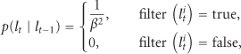
We only rely on direct arrivers and leavers information from the mobile seed. Thus, the filter condition of sample location $l_t$ is:

$\begin{array}{cc}\hfill \hspace{0.17em}\hspace{0.17em}\text{filter}\hspace{0.17em}\hspace{0.17em}\left(l_t^i\right)=& \left(d\left({\text{seed}}_c,n\right)\le r,\hspace{0.17em}\hspace{0.17em}d\left({\text{seed}}_p,n\right)>r\right)\hspace{0.17em}\hspace{0.17em}\text{or}\hfill \\ \hfill & \left(d\left({\text{seed}}_c,n\right)>r,\hspace{0.17em}\hspace{0.17em}d\left({\text{seed}}_p,n\right)\le r\right),\hfill \end{array}$

(8)

where ${\text{seed}}_c$ represents current location of seed, ${\text{seed}}_p$ represents previous location of seed, and the n represents the location of the unknown node.

The weight of sample is determined by the filter condition:

$w_t^{\prime i}=\{\begin{array}{cc}1,\hfill & \hspace{1em}\text{filter}\hspace{0.17em}\hspace{0.17em}\left(l_t^i\right)=\text{true},\hfill \\ 0,\hfill & \hspace{1em}\text{filter}\hspace{0.17em}\hspace{0.17em}\left(l_t^i\right)=\text{false}.\hfill \end{array}$

(9)

After computing the weight of the sample using (9), the weights are normalized to make sure that the sum of the weights of the samples is equal to one. The ith sample is normalized as

$w_t^i=\frac{w_t^{\prime i}}{{\sum }_{j=1}^N{w}_t^{\prime j}}.$

(10)

Resampling

In this step, each node computes a new sample set from its current sample set. Since the number of samples is kept fixed, in this step, a sample with a small weight has a lower chance of being selected, and a sample with a higher weight has a greater chance of being selected, and so many duplicates of that sample are likely to exist in the new sample set [4]. We adopt a systematic resampling algorithm [12] in this paper since it is simple to implement and minimizes the Monte Carlo variation.

4. Evaluation

We designed and implemented MA-MCL simulator with java language and also implemented MSL*, MSL, and ADO in this simulator and performed our simulations using it. For notational consistency with [4], we introduce the performance metrics used to compare localization algorithms and enumerate simulation parameters that are used in the experiments.

The key metric [4] for evaluating a localization algorithm is the accuracy of the location estimates or localization error. This is computed as follows:

$\text{Error}=\frac{1}{M}{\displaystyle \sum }_{i=1}^M\Vert l_i-R_i\Vert ,$

(11)

where M is the number of unknown nodes, $R_i$ denotes the real location of the ith unknown node and $l_i$ denotes the location estimate of the ith sensor where $i=1,\dots ,M$ . The errors shown in the simulation results are in terms of the radio range, that is, the errors shown are computed by dividing the error in (11) by the radio range of sensor node.

Our results were obtained using sensors randomly distributed in a 10 units × 10 units square field. We set ideal radio range $r=3$ in our experiments. The node density, $n_d$ , is the average number of sensors in the neighborhood of an unknown node. In our simulations, we set $n_d=10$ , the number of samples for an unknown node $N=50$ , the parameter $\beta =0.1r$ in the prediction stage, the maximum speed of the mobile seed $v_{\max \hspace{0.17em}}=1.0r$ unless otherwise specified. Other simulation parameters of the unknown node are based on the Mica Z sensor node. The seed's movement is implemented using random waypoint mobility model [4, 10].

In this section, we first show the evaluation results about the properties of MA-MCL algorithms such as the maximum speed of the mobile seed, the number of samples for unknown node, the impact of parameters β, neighbor nodes, and noise environment impact. Then we compare the accuracy of MA-MCL, MSL, MSL*, and ADO algorithms under same or different parameters configuration.

4.1. Properties of MA-MCL

4.1.1. Convergence

Figure 2 shows the convergence of MA-MCL algorithm under five different $v_{\max \hspace{0.17em}}$ . In general, the faster the speed of the seed, the quicker the stable phase is reached. The faster the speed of the seed, the more the number of unknown nodes which the seed could contact with. As shown in Figure 2, the localization process can be divided into the initialization phase and the stable phase. (1) In the initialization phase, the estimate error decreases dramatically as new observations (the localization is improved by both the current observation and previous observations) are incorporated. (2) In the stable phase, the impact of filter and the seed's mobility reach some balance, and the estimate error fluctuates around a minimum value. When $v_{\max \hspace{0.17em}}$ is greater than or equal to $1.0r$ , the convergence of MA-MCL is particularly fast, and the curves of convergences are very close to each other. Thus, we set $v_{\max \hspace{0.17em}}=1.0r$ as the default parameters configuration.

Figure 2

Location convergence under different $v_{\max \hspace{0.17em}}$ of seed conditions.

4.1.2. Number of Samples

Maintaining more samples for the MCL algorithm can improve accuracy, but requires additional memory [4]. As a result, in practical application, we should select an appropriate value of smaller samples which does not affect the accuracy of localization. Figure 3 shows the impact of sample size on location accuracy. The estimate error drops rapidly at the beginning since a small number of samples cannot adequately reflect the probability distribution. The estimate error is fairly stable after sample size equal to 50, and the accuracy improves only minimally by increasing the number of samples to 100 when $v_{\max \hspace{0.17em}}$ is greater than or equal to 0.6r. Hence, MA-MCL is efficient in both memory and computation when the number of sample is close to 50. Thus, consider saving memory and achieve good accuracy, we choose 50 as default samples value.

Figure 3

Impact of sample size.

4.1.3. Parameter β in Prediction Step

Figure 4 shows the impact of parameter β on location accuracy. If    $\beta =0.01r$ , that is, all samples of the unknown node always maintian minor changes in prediction step when its filter condition is met. As a result, it cannot provide enough variability in choosing new samples. When we increase the value of β to $0.05r$ or $0.1r$ , the convergence and accuracy have been improved significantly. As we continue to increase the value of β to $0.3r$ , convergence is improved correspondingly. The accuracy is not improved when localization reaches the stable phase, however. That is to say, the larger value of    $\beta$ will provide enough variability in choosing new samples, but increase the amount of uncertainty in the location estimates. Thus, there is a tradeoff involving β: we adopt $\beta =0.1r$ as default values.

Figure 4

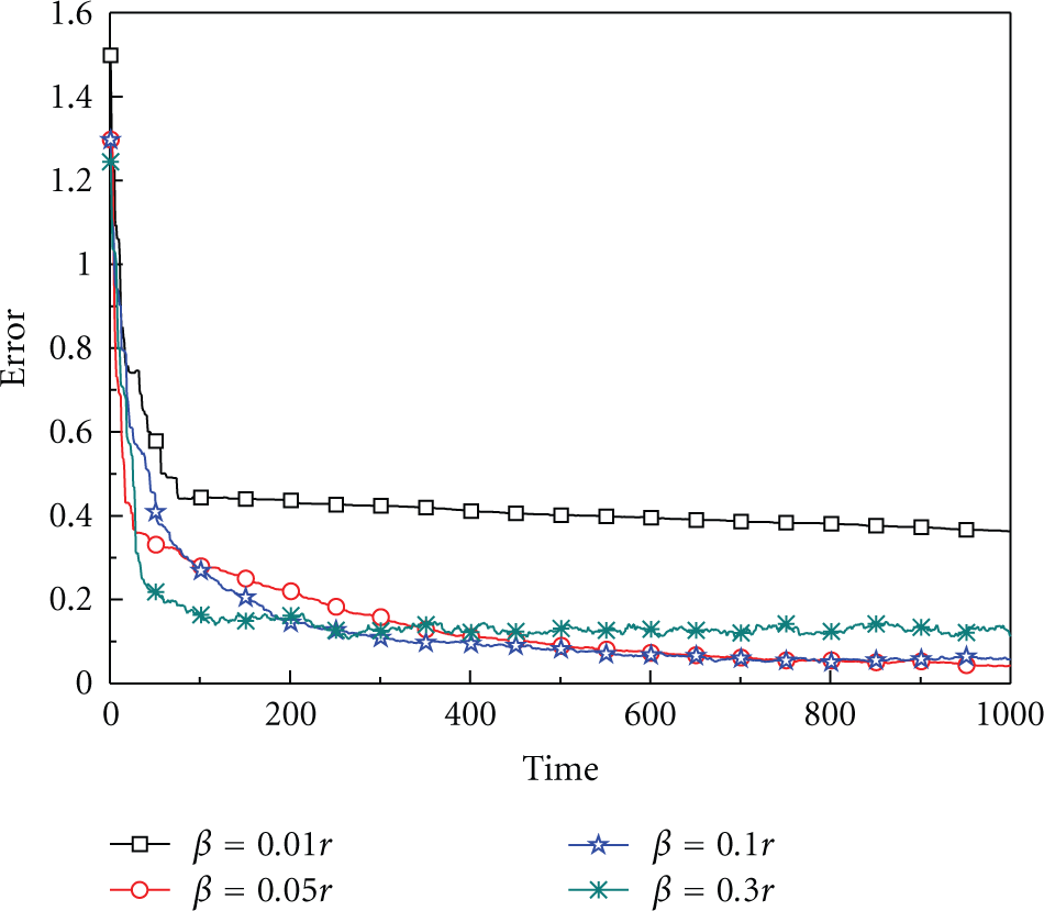
Impact of parameter β.

4.1.4. Neighbor Node

The number of observations to the unknown node in mobile seed-assisted approach is equal to the number of constraints from static neighbor seeds of the unknown node, that is, the number of observations in mobile seed-assisted approach are equal to the node density, $n_d$ . As a result, if the number of observations from the mobile seed to the unknown node is larger than $n_d$ , the neighbors'observation will not improve the precision of the unknown nodes. Figure 5 gives five test results about 10 unknown nodes which obtain the number of observations from mobile when we set the time of seed moving as 1000 time step to achieve stable phase with all default configurations shown in the third paragraph in Section 4. As shown in Figure 5, with these default configurations the number of observations from the mobile seed to the unknown node is always larger than default $n_d$ . Thus, MA-MCL with these configurations will not adopt the neighbor node observations.

Figure 5

The number of observations.

4.1.5. Noise Environment

All of our previous experiments assumed an ideal environment where location sensory data are not influenced by irregular radio range and any receiver within the radio range of sender will hear the packets from that sender. Here, we consider more realistic radio model, that is, the unknown node within radio range of the seed will not hear a location announcement (such as network collisions or missed packages) from that seed at some time. We use degree of irregularity (DOI) [10] to denote the maximum radio range variation in the direction of radio propagation. For example, if DOI = 0.1, then the actual radio range in each direction is randomly chosen from ( $0.9r$ , $1.1r$ ). Figure 6 shows six different DOI scenarios. The convergence and accuracy of MA-MCL are not substantially affected. That is to say, MA-MCL algorithm is robust and works well in the noise environment.

Figure 6

Noise environment.

4.2. Comparison of Different Algorithms

In order to compare different algorithms under the same conditions, MSL* and MSL in our evaluation will only use a single mobile seed for localization.

MA-MCL relies on direct arrivers and leavers information from the mobile seed, that is, it combines 1-hop and 2-hop seed position restriction at the same time. MSL* and MSL only adopt 1-hop connectivity restriction. Thus, in theory, the precision obtained by MA-MCL are twice as high as it obtained by MSL* or MSL. ADO adopts direct arrivers and leavers information, but it is not a recursive method. Obviously, compared to MA-MCL, the accuracy of ADO is very low. In the following sections, we give some experimental results about the comparison of different algorithms.

4.2.1. Accuracy

The graph in Figure 7 shows the accuracy comparison for MA-MCL, MSL*, MSL, and ADO. Figure 7 shows that the curve of ADO drops to a certain value, then to the horizon, because the seed in ADO moves in a straight line in the deployment area of a sensor network just once for a short time, and some unknown nodes are localized after the seed finished moving. Thus, as the time goes on, the average accuracy of all known nodes does not decrease. As shown in Figure 7, MSL* and MSL, these two curvatures of the curves are very close to each other. That is to say, in the mobile seed assisted localization scenario, the performance of the MSL*and MSL is no significant difference. Figure 7 also shows that the curves of MA-MCL and MSL* (MSL) are very similar to each other. As the time goes on, these curves reach the stable phase. MA-MCL shows nearly 50% better performance and nearly equal time of localization when compared to the MSL* and MSL. Thus, it can be seen from the figure that MA-MCL outperforms MSL*, MSL, and ADO.

Figure 7

Comparison of accuracy.

4.2.2. Speed of Seed

Figure 8 shows how the localization error varies with changing the speed of seed. Figure 8 shows that the faster speed of the seed, the worse accuracy of ADO. The faster speed of the seed, which just travels the whole deployment area of a sensor network only once, the more the number of unknown nodes, that are localized. When the speed of seed ( $v_{\max \hspace{0.17em}}$ ) is greater than $0.4r$ , the curves of MA-MCL, MSL*, and MSL will reach the stable phase. In this phase, MA-MCL always performs better than MSL* and MSL.

Figure 8

Speed of seed.

4.2.3. Density of Unknown Node

In this experiment we vary the density of unknown nodes. We set the time of seed moving as 1000 to achieve stable phase. As shown in Figure 9, the density of unknown node will not affect the accuracy of MA-MCL, MSL*, and MSL, just because the number of observations from the mobile seed to the unknown node is larger than $n_d$ , the neighbors' observation will not improve the precision of the unknown nodes.

Figure 9

Density of unknown node.

5. Conclusion

In this paper, we give an overview of related work for mobile-assisted and MCL approaches and we propose MA-MCL for WSNs. We conduct several simulations to evaluate our approach to show that the results outperform some other approach such as MSL*, MSL, and ADO. In future work, we continue to improve the accuracy to mobile-assisted localization based on research of the Monte Carlo methods. In addition, a number of practical factors will also be considered, and the practical factors may affect efficiency, accuracy, and flexibility of our localization approaches.