Context-Aware Scheduling of Distributed DL-Reasoning Tasks in Wireless Sensor Networks

Abstract

Wireless sensor networks (WSNs) provide a means to acquire lots of raw data from vast amounts of easy-to-deploy sensors. Ontologies facilitate structuring data into information and support automatic inference mechanisms. The combination of wireless sensor networks and ontologies can bring significant added value to intelligently process the raw data into meaningful information. In an ontology-based system, this process is referred to as description logics (DL) reasoning. However, the sensors might not be able to execute the reasoning process locally because of resource constraints. Additionally, the usage of the radio interface consumes a lot of power. Therefore, a balance has to be found between local processing and transmission towards the more powerful nodes. In this paper, we present our collaboration platform to bring together wireless sensor networks and distributed ontology A-Box reasoning. This platform should support the adoption of ontology-based methodologies and DL-Reasoning in a distributed setting. We detail a number of algorithms to optimise both bandwidth utilisation and power consumption. These algorithms have been evaluated on a real-life wireless sensor and mesh network test bed, namely WiLab.t. The results show that significant savings of up to 92% in terms of bandwidth utilisation can result from our approach.

1. Introduction

On the one hand, recent research initiatives have provided a boost towards the adoption of wireless sensor networks (WSNs). The relative low cost of such sensors and their adaptability to be used in different environments has resulted in massive deployments for a variety of use cases, oftentimes in the context of environmental monitoring. Because of the amount of sensor nodes being used in a typical wireless sensor network, the size of the dataset being produced by these sensors is huge. However, their use does not need to be confined to environmental monitoring. For instance, for the purpose of building automation and security, WSNs can provide an interesting solution.

On the other hand, the semantic web is gaining more and more adopters, and the usage of ontologies and reasoning in applications as a means to formally structure and analyse the data is increasing. Effectively, an ontology models a given domain in a graph structure. This graph contains the concepts present in the modelled domain, the relations between those concepts, and potentially classification axioms which specify generic knowledge about the domain. It can be exploited by the business logic of an application at a generic level of abstraction, by means of generic reasoning mechanisms. Moreover, ontologies allow not only to model the data in a formalised manner, but also to reflect the semantics of that data, thus the information and the knowledge of those systems. An example of such inference is root-cause analysis. Due to the foundation of ontologies in description logics (DL) [1], the models and description of the data in these models can be formally proven. The reasoning can also be used to detect inconsistencies in the model as well as infer new information out of the correlation of this data. This process is called DL-Reasoning. The most used and well-known language to describe ontologies is OWL (web ontology language) [2–4]. This technology allows for a common, formally defined and description logics supported data-format to be specified. Given the recently released W3C recommendation for OWL 2 [5], the successor of OWL, we can only conclude that this technology is very much actively used and continuously being enhanced and improved.

We propose a platform to support the collaboration between wireless sensor networks generating raw data and software modules structuring and analysing this data in an ontology-based manner. This approach brings advantages in data management for the end user application, by offloading some of the processing tasks towards the sink nodes of the sensor and mesh networks. The optimised scheduling of the processing tasks, which are called DL-Reasoning tasks, in this platform is important. We present a number of use cases indicating the importance to optimise network load in general and bandwidth utilisation in particular. Additionally, maximising the lifetime of remote, potentially battery-operated resources is introduced as well. In order to support these requirements, we have developed several algorithms and heuristics for the scheduling process of the reasoning tasks on the distributed nodes in the network. A balance has to be found between transmitting the ontology and its data to the back end and performing the reasoning in a centralised manner or executing the DL-Reasoning processes remotely and transmitting only the results to the client. Therefore, in this paper we detail the platform and present a number of scheduling algorithms. The first algorithm estimates the result set size of the reasoning tasks before the actual scheduling of those tasks on the nodes in the network is performed, taking into account general metrics of the specific ontology considered, in order to allow a second set of algorithms to optimise the network load or the power consumption of the remote nodes. These algorithms have been implemented in the platform and provide input to the actual scheduling of the DL-Reasoning tasks.

The proposed distributed DL-Reasoning approach presented in this paper has an important precondition. In the presented architecture, every ontology model on the distributed nodes is consistent and can be classified independently from the others in order to guarantee decidability of the reasoning process. This allows the instance realisation algorithm to draw complete conclusions in the scope of that particular deployment. The only exception is the adoption of a common vocabulary to link the individual ontologies together and to allow postreasoning integration of the reasoning results. Therefore, neither distributed consistency checking nor distributed T-Box classification crossing the boundaries of the distributed ontology models is taken into consideration. Section 3 details algorithms from related work to support distributed consistency checking and classification. The SPARQL query language is used to link the reasoning processes together and to coordinate the reasoning process from the back end [6, 7].

Many use cases can be identified where the injection of semantics and DL-Reasoning provides important added value to increase the usability and augment the user experience, particularly in distributed environments. However, the context in which reasoning can support application development does not need to be confined to that kind of end user applications. Reasoning can be applied to a variety of fields, such as intelligent network monitoring, environmental monitoring, or people guidance systems.

• (i)

A first use case handles the monitoring of multiple independent communication networks, for example, private home networks with the attached devices or even a home automation installation. A service provider can install an ontology model and DL-Reasoner on the access modem or router, and provide a service to the customer by monitoring the network behaviour and operation. Because each individual network deployment can have its own characteristics, it might be a good idea to push the model and the reasoning to the remote modem or router, so as to enhance the scalability and maintainability because the local knowledge is strongly coupled and kept with the individual deployment. Periodically, the service provider checks the reasoning interface on the modem to enquire about the current state of the network and any incipient or detected faults, so that a corrective action can be taken. These conclusions can thus be drawn in a generic manner without actually sending all measurement data to the service provider's back end. Alternatively, mechanisms can be provided as well to proactively inform the back end only in case such abnormal situations have been detected. In case of a network failure, back-up connection methods can be provided, although with limited available bandwidth or with high operational cost. Minimising the bandwidth utilisation is in this case required. Also in case of a local power failure, the adoption of power optimisation strategies can result in a longer uptime period for the devices which are powered through back-up batteries. An example ontology is “http://www.ida.liu.se/~iislab/projects/secont/Security.owl” that describes security technologies as a taxonomy and as countermeasures to protection goals. Many flavours of description logic exist. There is a naming convention, describing the operators used in the ontology model. In this case the ontology has a SHOIN(D) expressivity. More detailed information about these abbreviations can be found in [1]. Typical queries are mostly the retrieval of individuals which are classified according to specific constraints in the ontology model, such as defining specific vulnerabilities.

(ii)

A second use case concerns environmental monitoring. In this deployment, sensors acquire raw environmental data, for example, animal detection in forests. Preprocessing that data results in better information management and detection of potential dangerous situations. By modelling the specific problem domain in the ontology, the intelligence to draw the conclusions can be captured in a more generic manner. The model, together with a DL-Reasoner, can then be deployed on remote, but slightly more powerful nodes. In case certain conclusions are drawn by the reasoner, these can be notified to the back-end application, which in its turn can take appropriate measures. Because of the remote deployment, the likelihood of having broadband connectivity is low. Therefore, optimal usage of the available bandwidth is important. The remote nodes might also be powered by means of energy harvesters, requiring optimal usage of the limited available power. An example ontology with ALCHIN(D) expressivity is “http://protege.stanford.edu/junitOntologies/testset/animals-vh.owl”, modelling habitats and a wide range of animals. It allows to describe the observed animals and using the reasoner to classify the animal as a certain species.

(iii)

Processing people presence information can be considered as well. One can implement a centralised platform; however, every position or other information update would need to be transferred to this central system. If remote nodes, with specific responsibilities concerning local knowledge, would process the presence information, this communication overhead to the back-end can be reduced. This demonstrates the necessity for bandwidth optimisation strategies. In the situation of people guidance and crowd management situations, the information screens guiding the people can be influenced by the DL-Reasoner taking into account the current situation and the information modelled in the ontology for that particular area and situation. An ontology providing spatial concepts and property descriptions, such as for Transport, Religion, and Accommodation is “http://212.119.9.180/Ontologies/0.3/space.owl”. It has a ALCIF(D) expressivity.

(iv)

In the use case concerning person presence in city environments, the information taken into account can easily be extended. Some of the extensions can be the local restaurants or other places of interest. Therefore, the users of the system query the service for certain interesting places. If those persons additionally have some kind of personal ontology-based profile, this is also taken into account by the reasoner deployed on the individual node for the area the person is currently located in. This would then result, for example, in only those restaurants being returned which satisfy the interests of the end user. The reasoning could also be provided by a proprietary application on a smart phone of the end user. In order to extend the battery lifetime of the smart phone and to limit the amount of traffic exchanged, facilities need to be provided to optimise these metrics. Travel guides (“http://sites.google.com/site/ontotravelguides/Home/ontologies”) contain ontologies that enable inferring of user profile types based on user interests and activities. Likely, destination types are inferred based on the destinations data.

In [8], we have explored the adoption of an ontology-based methodology for building and wireless sensor network (WSN) monitoring, starting from an existing WSN ontology. One example definition modelled in the extension of this existing ontology specifies that a TMoteSky sensor node which has a sensor part that outputs at the same time zero as value for temperature, humidity and light intensity, or which does not produce anything at all is to be classified as faulty. However, using the same hardware and the same raw data, an additional definition for building automation has been inserted in the ontology model. In this definition, a room which has a system—that is, a TMoteSky—which in its turn has a sensor part that outputs a nonzero temperature value below $15{}^{\circ }\text{C}$ or above $25{}^{\circ }\text{C}$ , probably has a faulty HVAC system. These definitions are enhanced for every individual remote deployment, so as to take the local situation into account, for example, in a server room an upper threshold of $35{}^{\circ }\text{C}$ is still acceptable. Evolution over time is supported as well. For integration of new hardware, the addition of new ontology models and data providers suffices to include them in the monitoring workflow. After all, the specific definitions of the concepts against which the observations are checked to realise the correct Fault and Solution classification can be changed independently from the end monitoring application. When the reasoning process, monitoring the wireless sensor network, realises certain systems as faulty according to the constraints modelled in the Fault concept, it will automatically also realise the correct Solution instances, based on the definitions for the Solution concepts. Of course, the reasoner itself cannot take corrective action in the WSN. This is supported by an external application that uses the realised Solution concepts to invoke the corresponding operation on the nodes in the network, so as to correct the faulty behavior; for example, because the temperature in a certain office is too high, a technician could be sent on site to check the air conditioning system or otherwise certain valves could be openend by the monitoring system, so that additional cold air is redirected towards that particular office. Summarised is the adopted ontology design pattern, illustrated in Figure 2, enables a loosely coupled evolving ontology-based approach.

The research questions addressed in this paper can be summarised as follows. Firstly, how do we design the supporting collaboration platform for distributed DL-Reasoning in wireless sensor networks? Secondly, what are the necessary scheduling approaches to intelligently take decisions on raw input data in a distributed ontology-based and context-aware manner to increase the transparency of the information and include as much localised information as possible in a well-structured distributed approach? This general concept is illustrated in Figure 1. The last and main research question in this paper is: which optimisation algorithms are needed for the adoption of ontologies and more specifically for the optimised distribution of reasoning mechanisms within the specific nature of wireless sensor and mesh networks to support reasoning in constrained environments?

Figure 1

An example scenario where a number of different contexts have their own individual ontology models and reasoners for their own purpose, for example, monitoring, guidance, people presence. For every individual domain, a separate ontology and DL-Reasoner are available. A back-end service provider coordinates the reasoning processes. Upon request for information by clients, the back-end coordinator in the service provider's back office contacts the individual reasoners for each domain to retrieve the necessary information. The developed scheduling mechanisms in this back end are the focus of this paper.

Figure 2

Example inference chain to classify System individuals and infer certain Fault and Solution mechanisms.

The remainder of this paper is structured as follows. The following sections, Sections 2 and 3, present related work in the context of ontologies, wireless sensor networks in general, and data aggregation and fusion algorithms in particular. Also references towards the adoption of the semantic technology in WSNs are included. Section 4 introduces the distributed reasoning platform architecture which a.o. facilitates the automatic registration of the nodes in the platform with the central metamodel repository so as to facilitate the intelligent scheduling algorithms, while the developed optimisation and result set size estimation algorithms are presented in Section 5. An extensive evaluation of the algorithms is presented in Section 6. Finally, we conclude this paper in Section 7 with a number of general remarks and tracks for potential future research.

2. Background on DL-Reasoning

In this paper, we propose a context-aware distributed description logics reasoning platform for wireless sensor networks. A short, but comprehensive definition of an ontology, based on the definition in [9] is: “An ontology is a formal specification of an agreed conceptualisation of a domain in the context of knowledge description.” Accordingly, an ontology describes in a formal manner the concepts and relationships, existing in a particular system and using a machine-processable common vocabulary within a computerised system.

OWL [2–4], a modelling language for ontologies, consists of three sublanguages, each of them varying in their tradeoff between expressiveness and inferential complexity. They are, in order of increasing expressiveness: (i) OWL Lite: supports classification hierarchies and simple constraint features, (ii) OWL DL: OWL description logics, a subset providing great expressiveness without losing computational completeness and decidability and (iii) OWL Full: supports maximum expressiveness and syntactic freedom, however without computational guarantees. The syntax of OWL is based on XML (extensible markup language); the formal foundation for its semantics is based on Description Logics [1]. OWL is the natural evolution of several previous W3C recommendations, being XML, XML Schema, RDF, and RDF Schema.

Using one of the three sublanguage flavours of OWL, one can easily adapt to the required expressiveness. Arguably the most interesting sublanguage for many application domains is OWL DL, balancing great expressiveness with inferential efficiency. The efficiency is guaranteed by the underlying Description Logics [1]. Due to its foundation in Description Logics, OWL DL is also very flexible and computationally complete. Ontologies are considered as dynamic and evolving in time. As ontologies are also tailored towards the distributed nature of the Web, OWL additionally provides constructs for (de-)composition, extension, adaptation, sharing and reuse. On the other hand, OWL Lite has only limited expressive power, while OWL Full is undecidable and therefore not suited for many applications.

Recent research and standardisation efforts have taken OWL into a next level, OWL 2 [5]. In contrast to the earlier decomposition of the description logics in OWL Light, OWL DL and OWL Full, OWL 2 specifies a number of different profiles. According to [5], OWL 2 profiles can be more simply and/or efficiently implemented for a specific kind of application. Most profiles are defined by placing restrictions on the structure of OWL 2 ontologies. Each of the profiles is a trimmed down version of OWL 2 that trades some expressive power for the efficiency of reasoning. The profiles in OWL 2 are: (i) OWL 2 EL: useful in applications employing ontologies that contain very large numbers of properties and/or classes, (ii) OWL 2 QL: aimed at applications using very large volumes of instance data, and where query answering is the most important reasoning task, and (iii) OWL 2 RL: used for applications which require scalable reasoning without sacrificing too much expressive power.

In description of logic terminology, the T-Box contains the axioms defining the classes and relations in an ontology, while the A-Box contains the assertions about the individuals in that domain [10]. OWL, however, does not explicitly make this distinction because model and data can be mixed in the same description, but for clarification purposes it is still beneficial to make this distinction.

3. Related Work

For large scale and web scale reasoning, a promising initiative has been launched in the scope of the EU FP7 [11]. The aim of the Large-Scale Integrating Project LarKC is to develop the Large Knowledge Collider, a platform for massive distributed incomplete reasoning that will remove the scalability barriers of currently existing reasoning systems for the Semantic Web. Although certainly interesting and promising for reasoning in web scale deployments, the topic of this paper focuses on the integration of the semantic web technology in combination with wireless sensor networks.

We have studied previously how to enable distributed DL-Reasoning in resource unconstrained environments to reason over large ontologies. The details of the first iteration of the metamodel together with an evaluation which supports the case for distributed reasoning over large ontologies have been published in [6]. The agent architecture and the Java EE implementation details, namely the UML class and sequence diagrams, together with the detailed presentation of OTAGen, which has been used to generate multiple large ontologies, are presented in [7].

Additionally, the Berlin SPARQL Benchmark is presented in [12]. It defines a suite of benchmarks for comparing the performance of SPARQL-based systems across different architectures. Although not specifically aimed at deployments backed with a reasoner, this benchmarking suite could be adopted for the approach presented in this paper as well, since our approach also uses SPARQL queries to trigger the reasoning process.

An implementation that enables the distribution of the models and establishing semantic links between the concepts of the distributed models is DRAGO [13]. However, an optimal distribution of the reasoning tasks is not taken into account. Additionally, the implementation constrains the use of the reasoner software to its own extended implementation of the existing centralised Racer Pro reasoner [14]. The approach developed during this research does not require an extension to standard OWL DL reasoning and is as such not constrained to the use of a specific reasoner implementation.

In the WSN context, the recently launched SpitFire [15] project is worth mentioning. SpitFire stands for “semantic-service provisioning for the internet of things using future internet research by experimentation”. The aim of the project is to drastically lower the effort required for developing robust, interoperable, and scalable applications in the internet of things (IoT).

In the past, ontologies have been used as an efficient way to describe data and to facilitate a structured exchange of information between different stakeholders, mostly on the web. However, recently ontologies have found their way into more high-level information fusion where they provide a means to describe and reason about sensor data. In [16], a number of interesting use cases are presented, making the case to use ontologies in information fusion. Additionally, in [17], the KRAFT architecture is presented which supports such fusion of knowledge from multiple, distributed heterogeneous data sources. However, constraint solvers are used to process the information from the different sources. Our approach adopts a full description logics approach, as such avoiding additional transformation steps from the common ontology towards the constraint specification. Additionally, the communication between the agents in the KRAFT platform is supported by means of a proprietary messaging format. In our philosophy to use as many standardised technologies as possible, we have opted to adopt the SPARQL language as communication facilitator. There are a number of similarities as well. The services in the KRAFT platform can be compared to services provided by the platform presented in this work, for example, the Knowledge location services are similar to our metamodel, the Knowledge transformation services relate to the Aggregator modules while the Knowledge fusion services map onto the Reasoning Engine modules and Reasoning Distribution module in our platform. In contrast to the KRAFT architecture, the approach presented in this paper adopts a hierarchical strategy. In the hierarchical approach there is a single point of entrance into the system, which schedules the reasoning tasks on other nodes in the network. This creates a tree-based hierarchy of invocations where all underlying nodes have to report their conclusions from the reasoning process to the requestor on a higher level in the hierarchy.

A number of initiatives investigated previously how to incorporate semantic web technology in wireless sensor environments. A middleware for WSNs that exposes the functionality of the network as Semantic Web Services, so that applications can access its functionality through Web Services, is presented in [18]. Ontology-based data provisioning mechanisms for WSNs, in order to deal with varying applications, are presented in [19], while [20] defines a set of ontologies and accompanying architecture for knowledge sharing. In contrast, our approach brings the processing of and reasoning on the ontologies closer to the wireless sensor network itself, avoiding the need for extensive data transmission.

In [21] an overview is presented of data aggregation problems in energy-constrained sensor networks. The main goal of such algorithms is to gather and aggregate data in an energy efficient manner so that network lifetime is enhanced. Most of the techniques presented focus on the network setup, topology and data forwarding, and fusion techniques for sensor networks. The algorithms presented in [21] can be used in conjunction with the DL-Reasoning platform presented later in this paper in order to extend the battery lifetime of the (wireless) sensor network. However, because of the intensive computation required for DL-Reasoning, the reasoner will process the data only from the sensor network's sink on. Also in the context of existing algorithms for wireless sensor networks is [22]. Wiselib is an algorithm library that allows for simple implementations of algorithms onto a large variety of hardware and software. This is achieved by employing advanced C++ techniques such as templates and inline functions, allowing to write generic code that is resolved and bound at compile time, resulting in virtually no memory or computation overhead at run time.

The research detailed in this paper differentiates with the aforementioned related work in a number of ways. Firstly, our approach brings DL-Reasoning towards embedded and constrained devices. Secondly, the designed platform facilitates the distribution of knowledge and the cooperation of individual coordinated distributed reasoners. Lastly, the presented coordination process takes into account the context, that is, the location of the ontologies, as well as the resource and network characteristics, in which it needs to schedule the DL-Reasoning tasks.

4. Distributed DL-Reasoning Architecture

This section introduces the distributed DL-Reasoning platform and its support for the context-aware scheduling of DL-Reasoning tasks. The platform provides a number of specific modules to facilitate the deployment on wireless sensor and mesh networks.

4.1. Overview of the DL-Reasoning Architecture for Wireless Sensor Networks

The goal of the distributed DL-Reasoning platform is to be able to use description logics in a distributed wireless sensor environment. Previous research focused on system monitoring; more specifically, we deployed this platform for the monitoring of the IBBT WiLab.t infrastructure [23]. In this context, the constraints modelled in the ontology define abnormal situations in the behaviour of the nodes of the testbed. Additionally, by doing this in a distributed setting, we can easily model specific individual environmental characteristics in the ontology responsible for that section of the testbed. It is clear that similar deployments can be done for other use cases as well.

An overview of the complete architecture is given in Figure 3. For the presented scheduling optimisation, the developed algorithms have been implemented in the Scheduler component. This component in the Reasoning Distribution Module of the overall platform coordinator schedules given DL-Reasoning tasks on the specific nodes in the network according to certain scheduling algorithms or heuristics using certain context parameters.

Figure 3

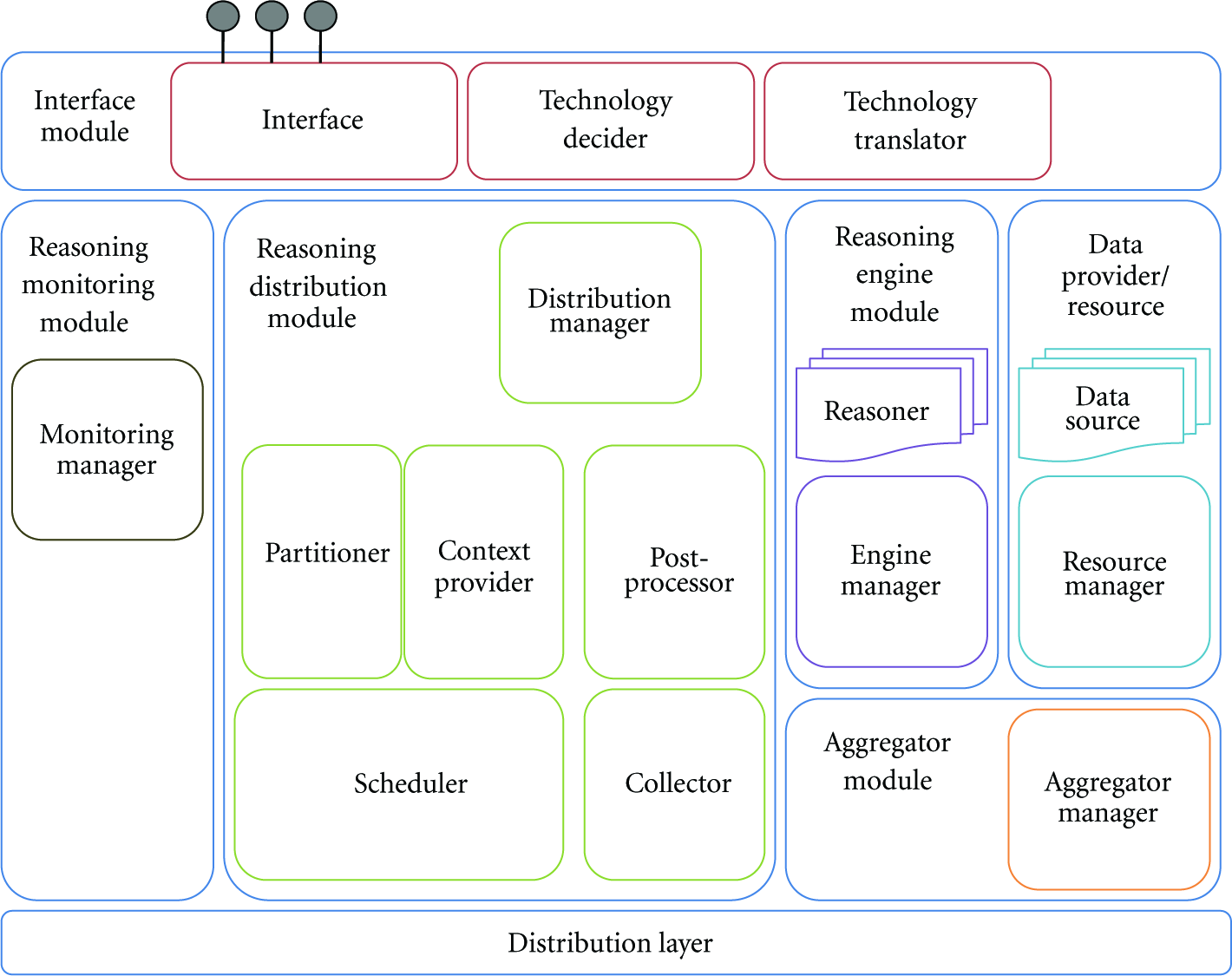
Extended ontology-based agent collaboration platform.

In the context of the interworking with wireless sensor networks, a few modules are of prime importance. The Data Provider/Resource Module will collect the data from the resources on which it has been deployed or for which it is responsible and feed it to the Aggregator Module. Upon request of the Reasoning Engine Module, the Aggregator Module will feed this collected data to the reasoning process. This way of working allows including sensor devices in the workflow, by means of sensor information generated from the Data Provider/Resource Modules deployed on the sensor devices. The deployment of this architecture involves a heterogeneous set of hardware, ranging from TMoteSky [24] sensors with nesC [25] software components, over wireless mesh nodes, Alix [26] boards, running the Linux Voyage [27] operating system, towards back-end servers running the preprocessing, scheduling, and postprocessing tasks. The deployment of the components on the sensors and other devices in the network is illustrated in Figure 4. The type of the interfaces between the modules is indicated along the arrows linking those modules. The rectangles with the annotations Data, Reasoning, Aggregator, Distribution, Monitoring and Interface refer to the corresponding modules in the architecture. As a reference, the architecture is repeated in the upper right corner of the deployment (Figure 4).

Figure 4

Deployment overview of the monitoring platform components on the heterogeneous hardware.

4.2. Implementation Details

We have adopted as many standardised interfaces and technologies as possible. The interface between the client, coordinator, and reasoners is SPARQL. Therefore, any library capable of understanding this standard can be used. The underlying ontology models are OWL DL compliant, and therefore any OWL DL compliant reasoner could be adopted. However, the latter is mostly tightly coupled with the SPARQL library. The implementation of the client, the coordinator, and the reasoners is done in Java SE. The modules implemented on the TMoteSky sensors are proprietary and have been developed in nesC. They use sockets to communicate with the Java implemented modules.

4.2.1. The Data Components

Each node that contains an Aggregator Module needs to collect the appropriate data. To this end, each sensor node regularly gathers system statistics, network statistics, and measurement data. The information is sent at runtime and wirelessly over an IEEE 802.15.4 interface to a sensor node connected to the mesh node responsible for the reasoning on the data from that sensor node. The sensor nodes use a multihop approach whereby measured information is sent over intermediate nodes to reach the Aggregator Module. Each Aggregator Module contains a software component which regularly broadcasts sink notification messages [28]. These messages inform the other nodes in the network where they can find the sink, for example, the uplink to the Internet or the application. In our case the sink contains the Aggregator Module. Each sensor node receives a sink message checks if the hop count is lower than any previously received sink message. If it is, the notification is further forwarded by the node, and the address of the neighbour from which the sink message was received is used as the default next hop address when forwarding measured data. This way, each sensor node sends its information from neighbour to neighbour until the information reaches the nearest aggregator node.

4.2.2. The Reasoning Components

A number of reasoning components have been developed and deployed on more powerful mesh nodes. The reasoning modules impose more stringent requirements on the hardware running these components. Using the mesh nodes, reasoning components can be deployed to process the data in a more intelligent way. These reasoning modules, using standard reasoning software, such as Pellet [29], analyse the data using the ontology model to draw conclusions about the status of the nodes in the testbed.

4.2.3. The Coordinating Back-End Component

The architecture of the distributed reasoning engine containing the different modules is devised in such a way that the algorithms for the different parts of the process, such as the presented scheduling algorithms, can easily be exchanged. The scheduling algorithms include optimisation of bandwidth utilisation and power consumption and are detailed in Section 5. This feature is supported by the plugin-based implementation for the scheduling algorithms.

4.2.4. Autonomous Registration and Metamodel Population

The scheduling algorithms need a number of context metrics in order to decide where to schedule each reasoning task. Amongst others, these metrics include the endpoint address of the remote reasoning service, the ontologies being served by those services, average round trip times, average result set size, model size, reasoning times, transmission times. A complete overview of the collected variables can be found in Table 1.

Table 1

Context metrics populated by the remote reasoning nodes in the central metamodels.

Metric	Type	Example
The endpoint address of the service on the node	String	http://inode9.test:18141/
The URL of the ontology being served by the node	String	http://localhost/owl#
The total available memory of the node	Long	55,611,392 bytes
The current memory consumption of the node	Long	1,151,040 bytes
The average model transmission time	Long	4,082 milliseconds
The uplink speed of the node	Long	26,214,400 bytes/milliseconds
The average response time per known query	Long	870 milliseconds
The average size of the compressed result set size per query	Long	4,444 bytes
The size of the model	Long	744,112 bytes
The size of the compressed model	Long	2,222 bytes
The current load of the node	Int	1 request
The total amount of CPUs of the node	Int	1
The current CPU load of the node	Double	38%
The uptime of the node	Long	5,501,125 milliseconds
The timestamp of the last update of the metamodel	Long	1,284,557,312,986 ms Unix time

As has been presented in [7], an ontology is used to describe these context parameters in the form of a metamodel. The metamodel ontology represents both the structure (T-Box) as well as the contents (A-Box) of this metamodel. The metamodel contains the contextual information for the ontologies, the DL-Reasoning services and the network and node characteristics in the platform. One of the reasons for deciding to use an ontology to model the metamodel is its native extension support. Exactly this feature has enabled us to further develop the scheduling algorithms, using an additional set of new metrics, without completely revising the metamodel implementation. The metrics mentioned in Table 1 have therefore been included in an extended metamodel ontology. The most important part of the enhanced ontology is presented in Figure 5. This section of the metamodel ontology is used to store the metamodel metrics used for the scheduling algorithm. It shows the relationships between the ontology concepts (in curved rectangles) and their data type properties (in normal rectangles).

Figure 5

Diagram highlighting an important part of the extended version of the metamodel presented in [7], used to store the scheduling metrics.

After the initial startup, all metrics are inserted in the metamodel information service with their respective values. The endpoint address of this information service is statically configured at deploytime of the reasoning service on the remote mesh nodes. Subsequently, during the course of operation, these metrics are periodically updated in this central metamodel repository, so as to reflect the latest state of the node. This update process has been implemented by means of SPARQL/Update. SPARQL/Update is a W3C submission [30] which suggests an expansion of the SPARQL recommendation [31] in order to be able to remotely update a certain ontology. This mechanism is used in our setup to enable the remote reasoning nodes to update the values of the collected metrics in the central metamodel repository. An example of two such SPARQL/Update queries is given in Algorithm 1. The first query deletes the current size of the compressed result set for a given reasoning query, while the second inserts the new value, that is, 4,444 bytes, for this metric. Because SPARQL/Update does not allow updating a value in a single operation, a sequence of a deletion and insertion has to be executed. The reasoning query concerned in this example is SELECT ?x WHERE ?x rdf:type wsn:Fault. This query searches for all individuals realised to be of the type wsn:Fault. This is a concept in the application ontology and is defined by means of restrictions.

Algorithm 1: Sample SPARQL/Update queries to synchronise the metamodel with the up-to-date values for the context parameters reflecting the current state of the remote node, for example, the remaining battery power or the CPU usage. The first query deletes from the metamodel the value for the compressed result set size, for a remote reasoning node with the hostname address http://inode9.test:18141/ and query SELECT ?x WHERE ?x rdf:type wsn:Fault. The second query inserts the new value of the compressed result set size for the same query on the same remote node.

PREFIX mm: <http://www.owl-ontologies.com/metaModelDistRea.owl#>

PREFIX xsd: <http://www.w3.org/2001/XMLSchema#>

DELETE {

  ?query mm : hasCompressedResultSetSize ?resultSetSize}

WHERE {

  ?spec mm : hasHostname “http://inode9.test:18141/”   $\widehat{\hspace{0.17em}}\hspace{0.17em}\hspace{0.17em}\widehat{\hspace{0.17em}}$   xsd : string.

  ?spec mm : answersQuery    $?$ query.

  ?query mm : queryString

    “SELECT ?x WHERE $\{?$ x rdf : type wsn : Fault}”   $\widehat{\hspace{0.17em}}\hspace{0.17em}\hspace{0.17em}\widehat{\hspace{0.17em}}$   xsd : string.

  ?query mm : hasCompressedResultSetSize ?resultSetSize }

PREFIX mm: <http://www.owl-ontologies.com/metaModelDistRea.owl#>

PREFIX xsd: <http://www.w3.org/2001/XMLSchema#>

INSERT {

  ?query mm : hasCompressedResultSetSize “4444”   $\widehat{\hspace{0.17em}}\hspace{0.17em}\hspace{0.17em}\widehat{\hspace{0.17em}}$   xsd : long}

WHERE {

  ?spec mm : hasHostname “http://inode9.test:18141/”   $\widehat{\hspace{0.17em}}\hspace{0.17em}\hspace{0.17em}\widehat{\hspace{0.17em}}$   xsd : string.

  ?spec mm : answersQuery    $?$ query.

  ?query mm : queryString

    “SELECT ?x WHERE {?x rdf : type wsn : Fault}”   $\widehat{\hspace{0.17em}}\hspace{0.17em}\hspace{0.17em}\widehat{\hspace{0.17em}}$   xsd : string.

  ?query mm : hasCompressedResultSetSize ?resultSetSize    $\}$

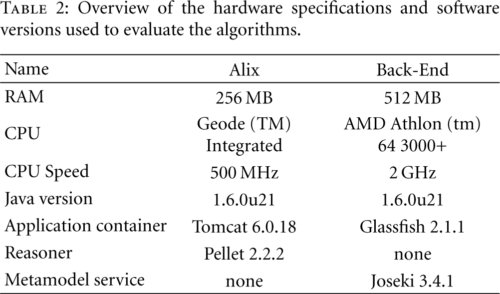
We conclude this subsection with an overview of the hardware specifications and software versions used to implement the algorithms. As reasoner we have used the well-known Pellet [29] DL-Reasoner implementation, which has been combined with a Jena [10] implementation to manage the ontology model, to invoke the reasoning processes and to execute the SPARQL queries. To facilitate the metamodel update process, a Joseki [32] service has been deployed. This detailed overview can be found in Table 2.

Table 2

Overview of the hardware specifications and software versions used to evaluate the algorithms.

Name	Alix	Back-End
RAM	256 MB	512 MB
CPU	Geode (TM) Integrated	AMD Athlon (tm) 64 3000+
CPU Speed	500 MHz	2 GHz
Java version	1.6.0u21	1.6.0u21
Application container	Tomcat 6.0.18	Glassfish 2.1.1
Reasoner	Pellet 2.2.2	none
Metamodel service	none	Joseki 3.4.1

5. Scheduling Algorithm Details

In Section 1, we presented a number of use cases indicating the importance to optimise network utilisation in general and bandwidth utilisation in particular. An optimisation in bandwidth utilisation can be achieved when scheduling the reasoning tasks on those locations which require the least amount of network traffic. This means that we have to compare the size of the result set of a given reasoning task with the size of the ontology model. This is the task of the MTSS, MTSSc, and MTSSdc algorithms, described in Section 5.1. However, the size of the model and the result set for particular queries changes over time. In order to adapt to this changing behaviour, we have adopted two approaches. The first approach uses a 1st order IIR filter. IIR stands for infinite impulse response and the origin of such a filter has to be found in the signal processing domain. It allows computing the output value by only considering the current input value as well as the output value from the previous run of the filter. The order equals the amount of previous output values to be considered, that is, one previous value in the case of a first order IIR filter (http://www.bores.com/courses/intro/iir/index.htm). The second approach consists of an estimation algorithm for the size of the result set, specifically developed for an ontology-based implementation. Additionally, maximising the lifetime of remote, potentially battery-operated resources was introduced as well. Starting from the estimated execution times for idling, reasoning and transmission and the characteristics of the devices used to reason on, we can choose the scheduling approach consuming the least amount of power. This is the approach implemented in the OPC algorithm. These algorithms will be detailed in the following subsections. Figure 6 gives an overview of the developed algorithms and how they collaborate to serve different aspects of the scheduling process.

Figure 6

Overview of the developed scheduling algorithms, illustrating their collaboration to serve different aspects of the scheduling process. The number between brackets refers to Algorithms 2–8.

Furthermore, we use the term reasoning task and query interchangeably. After all, to answer a certain query, the reasoner uses the domain ontology model, to classify the model and realise the data to formulate the correct answers to a given query. An example of this is the earlier mentioned query to retrieve all faulty sensors in the WSN, SELECT ?x WHERE ?x rdf:type wsn:Fault. The definition of a wsn:Fault specifies that a TMoteSky sensor node which has a sensor part that outputs at the same time zero as value for temperature, humidity, and light intensity, or which does not produce anything at all is to be classified as faulty. If the query is submitted to the reasoning engine module in our platform, this will trigger the reasoning process to realise all data in the ontology model and thus will find all TMoteSky sensors which satisfy this definition. The identifiers of those sensors are then returned in the result set of that query.

5.1. Bandwidth Optimisation

To reduce the bandwidth utilisation, a balance has to be found between, on the one hand, the amount of traffic needed for transmitting the entire unreasoned model and its data from the remote nodes to the back-end server and, on the other hand, executing the reasoning process on the remote nodes and transmitting the results to the back end. For this optimisation, we have developed one base algorithm with two extensions. These are presented in the following subsections.

5.1.1. Minimal Transmission Size Selection (MTSS)

In the base algorithm, MTSS, we compare the size of the complete ontology with the estimated size of the result set for that particular query. The initial situation, where an indication of the result set size is not yet available, is treated separately. Compared to the main operation of the algorithm, that is, where the size of the result set is adapted by means of applying a 1st order IIR filter ( $y[n]=0.5x[n]+0.5y[n-1]$ ) on the value from the current execution, the initial startup directly assigns the first result set size as the currently estimated value. In the formula, $x[n]$ represents the value of the result set size measured in the current execution, $y[n-1]$ contains the previously estimated result set size, while $y[n]$ is the new estimated result set size to be used in the next round of scheduling. This is the value as calculated by the 1st order IIR filter.

5.1.2. Minimal Transmission Size Selection, Using Compression (MTSSc)

The second algorithm, MTSSc, builds further on the mechanism of the MTSS algorithm. However, instead of transmitting the model or the result set in plain text, a compression algorithm is now used. Compression typically reduces the amount of transmitted data by a significant amount, of course at the cost of more processing. We have used the Java built-in compression mechanism, namely java.util.zip.GZIP.

Apart from the compression, there is another subtle difference with MTSS, namely the fact that the size of the result set is not updated anymore in case the query is executed in the back end. We think the overhead of first compressing the result set in order to enable an adaptable estimation of the result set in both cases is too large compared to the gain in case the result set size variable is updated only when the query is executed remotely.

5.1.3. Minimal Transmission Size Selection, Using Compression and Differences (MTSSdc)

In the second extension of the algorithms to minimise the bandwidth utilisation, MTSSdc, an optimisation has been implemented for the complete model transmission. After all, consecutive transmissions of the model oftentimes involve the transmission of many duplicates in the data. Therefore, the algorithm has been amended in such a way that the localNode, that is, the back-end server, caches a copy of the model contained in the remoteNode. In order to execute the query on the back end, the cached copy of that model on the back end now only needs to be updated with the difference between the previous transmission and the current. Therefore, it only involves the transmission of the updates on that particular model, further referred to as the differences of the model. In this third algorithm, which is presented in detail in Algorithm 2, variable $i_{\text{dc}}$ represents the 1st order IIR filter modified size of the compressed result set for a given query. Variable $k_{\text{dc}}$ represents the size of the compressed difference of the model starting from the latest transmission. The index dc refers to the differences and compression mechanism used in this algorithm. Finally, variable m contains the URL of the ontology model considered in the given query.

Algorithm 2: MTSSdc: Minimising bandwidth utilisation by adaptively scheduling the location of the reasoning task, using GZIP Compression and the transmission of model differences.

(1)                           ⊳ init:

(2) localModel←null

(3) m← metaModel.getModelForQuery(query)

(4) $i_{\text{dc}}$ ← 0

(5) $K_{\text{dc}}$ ← metaModel.getCompressedModelSize(m)

(6)                           ⊳ body:

(7) if $i_{\text{dc}}$ = 0 then

(8)   compressedResultSet = remoteNode.executeCompressedSPARQLQuery(query)

(9)   resultset = localNode.decompressResultSet(compressedResultSet)

(10)   $i_{\text{dc}}$ ← sizeOf(compressedResultSet)

(11) else

(12)   if   $i_{\text{dc}}$ ≤ $K_{\text{dc}}$   then

(13)    compressedResultSet = remoteNode.executeCompressedSPARQLQuery(query)

(14)    resultSet = localNode.decompressResultSet(compressedResultSet)

(15)    $i_{\text{dc}}$ ← (sizeOf(compressedResultSet) + $i_{\text{dc}}$ )/2

(16)  else

(17)   if  localModel = null then

(18)     compressedLocalModel = remoteNode.transferCompleteCompressedModel(m)

(19)     localModel = localNode.decompressModel(compressedLocalModel)

(20)     resultSet = localNode.executeSPARQLQuery(localModel, query)

(21)   else

(22)     compressedLocalDifference = remoteNode.transferCompressedModelDi_erence(m)

(23)     localDifference = localNode.decompressDifference(compressedLocalDifference)

(24)     addStatements(localModel, getAddedStatementsOf(localDifference))

(25)     removeStatements(localModel, getRemovedStatementsOf(localDifference))

(26)     resultSet = localNode.executeSPARQLQuery(localModel, query)

(27)      $K_{\text{dc}}$ ← sizeOf(compressedLocalDifference)

(28)   end  if

(29)  end  if

(30) end  if

(31) return  resultSet

We have chosen to implement the initial startup on the schedulers side, that is, before the mechanism of differences transmission can start, an initial transmission of the complete (compressed) model is to be completed.

5.2. Result Set Size Estimation (RSSE)

One of the disadvantages with the 1st order IIR filter used in the previous scheduling algorithms, executed in the back end, is that in the initial startup phase of the scheduling process, each of the potential scheduling outcomes has to be performed once, in order to collect the necessary metrics to support future executions. Moreover, this startup phase has to be performed for every new query offered to the system. To replace the reactive startup phase of the scheduling process with a proactive one, we developed an algorithm to estimate the size of the result set given a particular incoming query, based on the metrics of the complete ontology model. Of course, this estimation should be completed without actually executing the entire query. Therefore, the algorithm presented in this subsection calculates the upper boundary of the result set size, based on the amount of concepts, instances and properties present in the ontology model. In RSSE, variable δ represents the estimated upper bound of the result set size. For readability, the presentation of the algorithm is split up in several consecutive blocks. The first part presented in Algorithm 3, RSSE(Init), describes the initialisation phase of the RSSE algorithm. During the course of the RSSE algorithm, the tuple map variableCounts contains the estimated result set size for a single variable at any given time.

Algorithm 3: RSSE(Init): Estimation of the upper bound of the result set size—Initialisation phase.

(1)                             ⊳ init:

(2) long δ← 1;

(3) Individual s;

(4) Property p;

(5) Individual o;

(6) Map<String, Integer> variableCounts = new HashMap<String, Integer>();

(7) Map<String, Integer> propertyCounts = new HashMap<String, Integer>();

(8) Map<String, Integer> typeCounts = new HashMap<String, Integer>();

(9) OntologyModel model;

(10)                            ⊳ body:

(11) for  all  property← properties in model do

(12)   propertyCounts.put(urlOf(property), getPropertyCount(model, property));

(13) end  for

(14) for  all  concept← concepts in model do

(15)   typeCounts.put(urlOf(concept), getIndividualsCount(model, concept));

(16) end  for

(17) for  all  variable ← variables in query do

(18)   variableCounts.put(variable, maxValueOf(Integer));

(19) end  for

Algorithm 4, RSSE(Estimation), presents the second part of the RSSE algorithm. In this part, every triple pattern in the query is analysed independently.

Algorithm 4: RSSE(Estimation): Estimation of the upper bound of the result set size—Estimation phase.

(20) for  all triple← triples in query do

(21)   count← 0

(22)    s← subjectOf(triple);

(23)    p← predicateOf(triple);

(24)    o← objectOf(triple);

(25)    if  p NOT variable && s NOT variable && o NOT variable then

(26)              ⊳ Do nothing as additional solutions cannot

(27)              ⊳ from matching a triple without variables.

(28)    else  if  p NOT variable && s NOT variable && o IS variable then

(29)                  ⊳* stands for a wildcard. As such the triples are count,

(30)                 ⊳ matching the subject and the predicate.

(31)    count← sizeOf(listStatements(s, p, *));

(32)    replaceVariableCount(count, o);

(33)    else  if  p NOT variable && s IS variable && o NOT variable then

(34)    count← sizeOf(listStatements(*, p, o));

(35)    replaceVariableCount(count, s);

(36)    else  if  p NOT variable && s IS variable && o IS variable then

(37)    count← sizeOf(listStatements(*, p, *));

(38)    replaceVariableCount(count, s, o);

(39)    else  if  p IS variable && s NOT variable && o NOT variable then

(40)    count← sizeOf(listStatements(s, *, o));

(41)    replaceVariableCount(count, p);

(42)    else  if  p IS variable && s NOT variable && o IS variable then

(43)    count← sizeOf(listStatements(s, *, *));

(44)    replaceVariableCount(count, p, o);

(45)    else  if  p IS variable && s IS variable && o NOT variable then

(46)    count← sizeOf(listStatements(*, *, o));

(47)    replaceVariableCount(count, s, p);

(48)    else  if  p IS variable && s IS variable && o IS variable then

(49)    count← sizeOf(listStatements(*, *, *));

(50)    replaceVariableCount(count, s, p, o);

(51)    end  if

(52)    for  all  variable← variables in query do

(53)       δ←δ × get(variableCounts, variable);

(54)    end  for

(55) end  for

(56) returnδ

The update procedure, RSSE(Update) of the current size of a result set for a given variable with the new information being discovered for the current query triple pattern analysis, is given in the procedure replaceVariableCount in Algorithms 5, 6, and 7.

Algorithm 5: RSSE(Update 1): The update process of the tuple map with the minimum of count and the currently estimated result set size for variable.

(1) procedure  replaceVariableCount(count, variable)

(2)  currentCount← get(variableCount, variable);

(3)  put(variableCounts, variable, min(currentCount, count));

(4) end  procedure

Algorithm 6: RSSE(Update 2): The update process of the tuple map with the minimum of count and the currently estimated result set size for variable1 and variable2.

(1) procedure  replaceVariableCount(count, variable1, variable2)

(2)  currentCount1← get(variableCount, variable1);

(3)  currentCount2← get(variableCount, variable2);

(4)  minimumCurrentCount← min(currentCount1, currentCount2);

(5)  put(variableCounts, variable1, min(minimumCurrentCount, count));

(6)  put(variableCounts, variable2, min(minimumCurrentCount, count));

(7) end  procedure

Algorithm 7: RSSE(Update 3): The update process of the tuple map with the minimum of count and the currently estimated result set size for variable1, variable2 and variable3.

(1) procedure  replaceVariableCount(count, variable1, variable2, variable3)

(2)   currentCount1← get(variableCount, variable1);

(3)   currentCount2← get(variableCount, variable2);

(4)   currentCount3← get(variableCount, variable3);

(5)   minimumCurrentCount← min(currentCount1, currentCount2, currentCount3);

(6)   put(variableCounts, variable1, min(minimumCurrentCount, count));

(7)   put(variableCounts, variable2, min(minimumCurrentCount, count));

(8)   put(variableCounts, variable3, min(minimumCurrentCount, count));

(9) end  procedure

The algorithm calculates the upper bound of the result set size, by analysing the contents of every triple pattern in the query. If the pattern has a variable for either subject, predicate, or object, the model is searched for all triples which have the nonvariable parts of the triple pattern from the query bound and a wildcard is used for the part of the query triple pattern which has an unbound variable. The size of the set with these matching triples is then compared with the currently known amount of matching triples for the given variable in the query triple pattern, for example, because the variable was already used in a previous query triple pattern. If the new size is smaller than the previous one, the value is replaced with the current size. This is implemented by the procedure ReplaceVariableCount. After all, the queries are conjunctive in nature, and therefore only the smallest set determines the ultimate upper bound of triples matching that particular variable.

A similar principle has been implemented in case more than one part of the triple pattern contains variables. In this situation, the size of the set of triples in the model matching the triple pattern is compared with all variables in the triple pattern. However, an additional minimisation step is performed; that is, the lowest of the existing sizes currently registered with the variables is mutually assigned to all variables. This is represented in Algorithm 6 for 2 variables and Algorithm 7 in the case 3 variables exist in the query pattern.

The actual calculation of the final estimation is done after the analysis phase. Once all query triple patterns have been reviewed, a map is obtained containing for each variable the minimum amount of triples potentially matching the triple pattern in the query. Because the algorithm does not take into account the semantics of the query, it cannot assume any interrelation between the variables in the query. Therefore, the multiplication of the minimum count of potentially matching triples for each variable is taken. This is shown at the end of Algorithm 4, lines 52–54.

In Section 6, we have used ontology models and SPARQL queries generated by OTAGen [33]. These ontologies are in line with existing ontologies for location-aware services, such as for travel or touristic information. An example query using such ontology models, illustrating the motivation for the RSSE and MTSS algorithms, is given below. The purpose of the query is to ask for all possible combinations for an evening out with friends, consisting of a dinner, some evening activity and a final drink in a pub.

PREFIX dinner: <http://localhost/owl/dinnerOntology#>

PREFIX act: <http://localhost/owl/activityOntology#>

PREFIX pubs: <http://localhost/owl/pubOntology#>

PREFIX rdf: <http://www.w3.org/1999/02/22-rdf-syntax-ns#>

SELECT  {

 ?dinner ?activity ?pub  

}  WHERE  {

 ?dinner rdf : type dinner : ItalianRestaurant.

 ?activity rdf : type act : Cinema.

 ?pub rdf : type pubs: IrishPub

}

Due to the triple matching algorithms implemented in SPARQL processors, the result set containing all matching possibilities, can potentially be larger in transmission size compared to the size of the serialised model. However, depending on the amount of data in the A-Box of the ontology, not included in the query detailed above, the model is oftentimes larger than the size of the results set size. This depends on the selectiveness of the query and the amount of data in the ontology model not related to the query. An optimal scheduling of the reasoning processes, minimising the bandwidth utilisation, is important when a user wants to query the city-service from the example, using his PDA or smartphone, to retrieve the information while walking in the city. This ensures the most optimal use of the commercial network for which the user pays a subscription or pay-as-you-go fee and oftentimes does not have unlimited access to.

5.3. Optimisation of the Power Consumption (OPC)

The last algorithm, OPC, focuses on a different optimisation metric, namely, the power consumption of the remote nodes. In the situation where those nodes are deployed as sinks for a wireless sensor network in a remote environment, the chance of having these operated by batteries, or some other kind of limited power source, is not unrealistic. Therefore it is important to schedule the reasoning or transmission tasks in such a way as to minimise the consumed energy. To enable this optimisation, we have defined three key metrics, namely the power consumption during idling (γ), during reasoning (α), and during transmission (β). The invocation and processing flow of both approaches, that is, the remote reasoning or the transmission and back-end reasoning are graphically presented in Figures 7 and 8. The invocation phase where the scheduler either requests a transmission or a reasoning task to be performed is considered a constant time delay. Therefore, the invocation arrow is drawn completely vertical.

Figure 7

Example time diagram illustrating the invocation and processing flow in the case of reasoning on the remote node.

Figure 8

Example time diagram illustrating the invocation and processing flow in the case the model is transferred from the remote node to the back-end. Additionally, the back-end reasoning process is included as well.

The details of the OPC algorithm are presented in Algorithm 8. In the evaluation we have conducted a theoretical study towards the optimal values of those three metrics, and this for a number of typical reasoning tasks. In the OPC algorithm, variable ϵ(rr) contains the estimated power consumption of the remote node in case the reasoning is performed on the remote nodes. Variable ϵ(lr) on the other hand contains the estimated power consumption of the remote node in the case of transmission of the model and reasoning on the back end.

Algorithm 8: OPC: Optimising power consumption by approximation of the scheduling options.

(1)                           ⊳ init:

(2) $\mathrm{\Delta }{t}_{\text{ctr}}$ ← metamodel.getAverageComputationTimeRemoteReasoning(query)

(3) $\mathrm{\Delta }{t}_{\text{ttr}}$ ← metamodel.getAverageTransmissionTimeRemoteReasoning(query)

(4) $\mathrm{\Delta }{t}_{\text{stm}}$ ← metamodel.getAverageSerialisationTimeModel(query)

(5) $\mathrm{\Delta }{t}_{\text{ttm}}$ ← metamodel.getAverageTransmissionTimeModel(query)

(6) $\mathrm{\Delta }{t}_{\text{rttr}}$ ← metamodel.getAverageRoundTripTimeRemoteReasoning(query)

(7) $\mathrm{\Delta }{t}_{\text{rttm}}$ ← metamodel.getAverageRoundTripTimeLocalReasoning(query)

(8) α← metamodel.getPowerConsumptionDuringComputation()

(9) β← metamodel.getPowerConsumptionDuringTransmission()

(10) γ← metamodel.getPowerConsumptionDuringIdleTime()

(11)                          ⊳ body:

(12) ϵ(rr) ←  α×   $\mathrm{\Delta }{t}_{\text{ctr}}$ + β×    $\mathrm{\Delta }{t}_{\text{ttr}}$ + γ× ( $\mathrm{\Delta }{t}_{\text{rttr}}$ −    $\mathrm{\Delta }{t}_{\text{ctr}}$ −    $\mathrm{\Delta }{t}_{\text{ttr}}$ )

(13) ϵ(lr) ←α×   $\mathrm{\Delta }{t}_{\text{stm}}$ +    $\mathrm{\Delta }{t}_{\text{ttm}}$ + γ× ( $\mathrm{\Delta }{t}_{\text{rttm}}$ −    $\mathrm{\Delta }{t}_{\text{stm}}$ −    $\mathrm{\Delta }{t}_{\text{ttm}}$ )

(14) ifϵ(rr) ≤ ϵ(lr) then

(15)  resultSet = remoteNode.executeSPARQLQuery(query)

(16) else

(17)  localModel = remoteNode.transferCompleteModel(m)

(18)  resultSet = localNode.executeSPARQLQuery(localModel, query)

(19) end  if  return  resultSet

In the implementation of this algorithm, we have used the first nonoptimised MTSS approach, that is, without compression or differences. Of course, any of the optimisation techniques described in the MTSSc or MTSSdc algorithms can be used as well. This would result in two new variants of the OPC algorithm, namely, the OPCc and the OPCdc algorithm.

The OPC algorithm uses the execution time as a metric to reflect the efficiency of the reasoning task. Heavy reasoning tasks will take a long time to complete. Therefore, the power consumption on the remote node will increase significantly and the OPC algorithm will unlikely schedule these reasoning tasks on the remote battery-operated sensor nodes. Of course, it is very important to design the ontology models as efficiently as possible. This could be checked beforehand by means of specific software, for example, Pellet Lint [29]. The efficiency of the reasoning task itself does not influence the scheduling algorithms presented in this section since only decidable DL-reasoning processes are considered as a precondition. Important to note is that the metrics of the reasoning processes are used by the algorithms to optimise certain metrics, such as bandwidth utilisation or power consumption. We believe that the presented algorithms are worthwhile to be developed and adopted for real-life sensor applications because of the optimisation of important metrics related to wireless sensor networks. This evaluation of this optimisation is presented in the following section.

6. Performance Evaluation

In this section, the evaluation of the algorithms is detailed. Firstly, a presentation of the evaluation setup is given, followed by the evaluation of the influence of the bandwidth optimisation approach on the scheduling decisions. The next subsection details the evaluation of the RSSE algorithm, and finally a theoretical study of the OPC algorithm is presented. Furthermore, previous research in [7] presents an evaluation of the overhead introduced by the platform and the cost it incurs to adopt the distribution mechanisms. This overhead study does not consider the running times of the scheduling algorithms evaluated in this section, but includes the processing of all other phases in the platform.

6.1. Evaluation Setup

6.1.1. Generated Ontology

Using OTAGen [33], an evaluation ontology has been generated. OTAGen facilitates the generation of ontologies and corresponding queries with specific characteristics, such as the amount of concepts, constraints, individuals, and so forth. The characterising metrics of this ontology correspond to those of the ontologies in the use cases. In contrast to those ontologies, which oftentimes do not have an A-Box readily available, OTAGen allows us to easily generate an A-Box for the corresponding T-Box as well as a number of queries, which can be used for evaluation and reasoning. The generated ontology is of ALCHOIN(D) expressivity, containing 62 concepts, 27 object properties, 41 data properties and 166 individuals. Additionally, 12 constraints have been defined in the ontology to increase the reasoning complexity.

6.1.2. Testbed Hardware

The ontology has been deployed, together with the reasoning components, on the hardware of the IBBT WiLab.t testbed. However, we have only used the iNodes—an Alix 3C3 device [26] running Linux Voyage [27]—and have not directly incorporated the wireless sensor nodes to generate real time data. Whether or not actual real time data is available in the model only influences variability of the reasoning outcomes, but not the scheduling as such. A picture of the hardware is shown in Figure 9(a), and a schematic overview of the testbed, illustrating a component break down of the nodes, is illustrated Figure 9(b).

Figure 9

The nodes in the WiLab.t testbed infrastructure.

6.1.3. Five Query Types

For the evaluation of the algorithms, five different SPARQL-queries of increasing result set size and amount of query triple patterns have been generated. Since we used OTAGen to create an evaluation ontology with similar characteristics to existing ontologies that facilitate use-cases for context-aware systems, the generated SPARQL-queries are realistic ones but do not have any semantic relevance as such. On the one hand, the SPARQL-queries with a small result set size represent situations where the context-aware systems ask very specific questions with high selectivity. Whether or not the constraints are specified within the queries, and thus have a large number of query triple patterns, or trigger the reasoning by means of constraints already present in the ontology, depends on the situation. One can either search for new information or request data according to already known constraints. This kind of queries is the most common one. The queries with a large result set size on the other hand represent less commonly asked questions—with a lower selectivity—and return lots of context information which can be used by the application for further processing. Each of those queries will be offered 50 times to the distributed reasoning platform. As such, a complete set of 250 queries is constructed. To get a clear view on the scheduling outcome, these 250 queries are executed sequentially, sorted according to increasing amount of query triple patterns. The details of the queries are given in Table 3. In the names of the queries the suffix of rs denotes the result set size and the suffix of tp details the number of query triple patterns to be matched.

Table 3

Characteristics of each of the five queries, generated by means of OTAGen for the evaluation of the scheduling algorithms. It indicates for every query the amount of triples to be matched and the amount of items returned in the result set for that query.

Query	Query triple pattern count	Result set count
q_rs44tp1	1	44
q_rs2166tp5	5	2,166
q_rs8100tp7	7	8,100
q_rs11664tp8	8	11,664
q_rs48384tp9	9	48,384

6.1.4. Evaluation Outline

In the following subsections the evaluation of the scheduling algorithms is presented. Section 6.2 evaluates the influence of the bandwidth optimisation strategies on the scheduling outcome of the back-end algorithms. First the influence of the MTSS algorithm is presented, followed by the extension of the MTSS algorithm with compression techniques (MTSSc algorithm) and the influence of the adoption of the model differences strategy (MTSSdc algorithm). Finally, an evaluation of the total consumed bandwidth for each of the three strategies is detailed. In Section 6.3, the evaluation of the RSSE algorithm by means of the LUBM [34] benchmark is presented. The performance evaluation is concluded with a theoretical study on the power optimisation algorithm OPC in Section 6.4.

6.2. Influence of the Bandwidth Optimisation Algorithms on The Scheduling Outcome

In this first evaluation paragraph, the influence on the scheduling outcome is examined. In particular the influence of bandwidth utilisation optimisation as implemented in the MTSS algorithm is examined. In the first graph presented in Figure 10, two values for the estimated bandwidth consumption have been plotted showing the estimated bandwidth utilisation for each of the first 150 queries, clustered in three groups of 50 identical queries. The result set sizes of five different queries have been evaluated, of which only the first three have been plotted in the graphs. The first value, indicated by the striped line, shows the estimated transmission size in case the complete model would be transferred to the back-end coordinator. The second value, indicated by the continuous line, represents the estimated size of the result set in case the reasoning is performed remotely on the Alix board. Because the MTSS algorithm learns the size of the result set during the course of operation, with every change of query—at position 1, 51, 101—the estimated result set size is reinitialised to 0. The scheduler chooses the option which consumes the least network traffic. This results in remote reasoning and result set transmission for the first query, and back-end reasoning with model transmission for the other queries. The switch-over point is indicated by the arrow on the graph. The actual values for the result set size are, respectively, 759; 374,846; 1,871,260; 2,822,871; 13,938,169 bytes. The serialised model is 93,014 bytes. Additionally, the actual bytes transmitted during the evaluation is plotted with the thin dotted line.

Figure 10

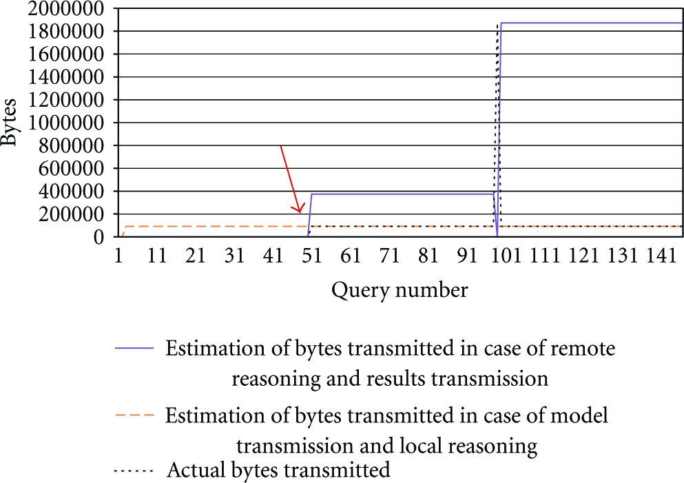
Scheduling overview with the estimation of the bytes to be transmitted in the initial situation where no additional measures have been taken to optimise network utilisation (MTSS algorithm).

Taking the graph from Figure 10 as reference point, the first optimisation—in the MTSSc algorithm—uses the GZIP compression mechanism to compress both the serialised model as well as the result sets of the individual queries. The influence on the values of either scheduling option, that is, remote or back-end reasoning, is presented in Figure 11. It can clearly be seen that the decisions being taken by the scheduler are not influenced by the use of compression techniques. The actual values for the result set size are now, respectively, 1,288; 57,176; 205,184; 278,336; 1,287,488 bytes and the size of the serialised model is now 47,808 bytes. This size of the serialised model is still smaller than the result set size for queries 2, 3, 4, and 5.

Figure 11

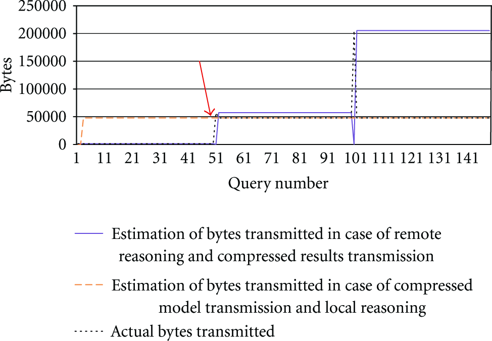
Scheduling overview with the estimation of the bytes to be transmitted in the situation where both the serialised model and the query result set are compressed to optimise network utilisation (MTSSc algorithm).

The switch-over point is still located at iteration 51, that is, the start of the second least complex query. The first query illustrates that an optimisation of bandwidth utilisation is achieved by distributing the reasoning either towards the remote or local nodes.

In the last bandwidth utilisation optimisation step, implemented by the MTSSdc algorithm, we have included the mechanism to transmit only the differences compared to the last transmission of the model. Therefore, we have added a fourth value on the graph to represent the estimated size of that compressed difference. This graph is presented in Figure 12. The interpreting principles of this graph remain the same, that is, still the scheduling option with the lowest transmission size will be chosen. Of course, as described in Algorithm 2, before the option of transmitting the differences can be chosen, it is necessary to transmit the entire model at least once beforehand.

Figure 12

Scheduling overview with the estimation of the bytes to be transmitted in the situation where both the serialised model as well as the query result set are compressed to optimise network utilisation. An additional value has been plotted to indicate the estimated transmission size in the case a local cache is used and only the difference with that cache is transmitted in a compressed manner (MTSSdc).

We can conclude that for query q_rs44tp1 it is still beneficial to execute the reasoning on the remote node and transmit the results to the requestor. The total size of the compressed result set is lower than the size of the compressed model differences. The switch-over point is located at position 51. This is the moment the second query starts being executed. From this moment on the size of the serialised differences of the model is lower than the size of the compressed result set. Should the size of the differences ever become larger than the actual transmission of the entire model, the scheduler will automatically decide to retransmit the entire model. The average size of the differences is 3,729 B compared to 47,808 B for the serialised and compressed model. This results in an average gain of 92.2%.

In a last evaluation concerning the bandwidth utilisation optimisation, the total amount of bytes transferred over the communication link in each of the three scheduling situations detailed above, is presented. To do this, the sum is made of the actual bytes transmitted according to the decided scheduling option. The values for each of the three strategies are, respectively, 36,901,369 B; 11,262,952 B; 2,623,468 B. This results in a cumulative net improvement of 69.48% and 92.89% in transmission size.

6.3. Evaluation of the Estimation of the Result Set Size

The second part of the evaluation, detailed in this subsection, presents the evaluation of the estimation of the result set size for a given model and SPARQL query. This corresponds to the RSSE algorithm, detailed in Section 5.2. Based on general metrics of the model, we calculate an upper bound of the result set size. In order to avoid any potential bias in the query generating strategy we implemented in OTAGen on the one hand and the result set size estimation algorithm on the other hand, we have used the LUBM [34] benchmark to evaluate the estimation algorithm. The results of the estimation algorithm are detailed in Table 4. This table details the estimated result set size, the fraction the estimated result set size represents compared to the actual result set size and the fraction of the estimation compared to the theoretical maximum result set size. This maximum is calculated according the number of individuals present in the model, the number of variables in the query and the assumption that each variable in a given triple pattern in the query does not have any relationship whatsoever with any of the other variables in the other query triple patterns. Given these preconditions, this theoretical maximum can be expressed as the number of individuals in the model raised to the power of the number of variables in the query. The algorithm estimates the number of variable bindings in the result set and not the actual serialised size of the result set. Therefore, this estimated binding count is multiplied with the average size of a serialised individual in the model. After all, according to the OWL standard, each instance reference is a (fully expanded) URL, of which the variation is only a few string characters, thus minimising the potential inaccuracy.

Table 4

Result set estimation results. Actual Fraction = EstimatedResultSetSize/ActualResultSetSize, TheoreticalMaximumFraction = TheoreticalMaximumResultSetSize/ActualResultSetSize.

Query	Estimated size	Actual fraction	Theoretical Maximum fraction
LUBM 1	922 B	1.25	$2.33·10^{-4}$
LUBM 2	431,970 B	$2.75·10^3$	0.11
LUBM 3	1,383 B	11.8	$3.49·10^{-4}$
LUBM 4	651,357,192 B	$4.35·10^4$	$3.25·10^{-11}$
LUBM 5	165,734 B	1.54	0.04
LUBM 6	1,795,648 B	1.54	0.45
LUBM 7	1,500,138	85.2	$2.21·10^{-5}$
LUBM 8	6,883,636,791 B	$2.39·10^3$	$5.9·10^{-6}$
LUBM 9	208,436,163,832 B	$2.63·10^6$	$1.79·10^{-4}$
LUBM 10	922 B	1.25	$2.33·10^{-4}$
LUBM 11	51,634 B	1.61	0.014
LUBM 12	51,864 B	13.6	$7.63·{10}^{-7}$
LUBM 13	231 B	0.76	$5.82·{10}^{-5}$
LUBM 14	1,363,678 B	1.53	0.34

As can be expected, the estimation algorithm performs best in situations where the number of variables is low and their mutual dependencies are limited. In the other cases, the reason for the sometimes excessive overestimation is the fact that semantically the algorithm cannot estimate the interrelation between the variables in the triple patterns of the query. Only a reasoner can do this, of course at a certain computational cost. By only analysing the individual triple counts, we can rapidly make an estimation of the result set size which can then be used as a quick input to the reasoning scheduling algorithm, however at the cost that some of the semantic relations between the query triple patterns are neglected.

Feeding back these results towards the earlier algorithms concerning the optimisation of bandwidth utilisation, the estimation results can be used to make a more educated initial estimation on the potential result set size in the case no previous executions of the query have been executed. In these situations, the algorithm would originally simply try each of the potential scheduling options. Instead, the estimation is now used in this initial phase and during the course of operation, the 1st order IIR filter mechanism will adapt the estimation rapidly towards the real result set sizes.

To evaluate the influence this estimation algorithm has on the initial reasoning scheduling decisions, both approaches, that is, with and without the estimation algorithm, have been compared. In this experiment, the optimisation algorithm MTSS is used as reference. Table 5 details the actual sizes of the result sets for each of the 14 LUBM queries as well as the estimated result set sizes according to the estimation algorithm presented earlier. The size of the entire serialised model is 8,426,139 bytes. Based on these numbers, the algorithm will choose the option which incurs the least amount of network traffic, according to the MTSS algorithm detailed in Section 5.1. The actual amount of bytes transmitted for the execution of this reasoning task is detailed in the fourth column. The decision is presented in the fifth column of the table—R stands for remote reasoning with result set transmission, T stands for model transmission and back-end reasoning.

Table 5

Influence of the result set estimation algorithm on the reasoning task scheduling decisions. The fourth column indicates the actual bandwidth utilisation as a result of the adoption of the RSSE algorithm.

Query	Estimated size	Actual size	Bandwidth utilisation	Decision
LUBM 1	922 B	740 B	740 B	R
LUBM 2	431,970 B	157 B	157 B	R
LUBM 3	1,383 B	117 B	117 B	R
LUBM 4	651,357,192 B	14,989 B	8,426,139 B	T
LUBM 5	165,734 B	107,496 B	107,496 B	R
LUBM 6	1,795,648 B	1,166,328 B	1,166,328 B	R
LUBM 7	1,500,138 B	17,609 B	17,609 B	R
LUBM 8	6,883,636,791 B	2,880,400 B	8,426,139 B	T
LUBM 9	208,436,163,832 B	79,299 B	8,426,139 B	T
LUBM 10	922 B	740 B	740 B	R
LUBM 11	51,634 B	32,103 B	32,103 B	R
LUBM 12	51,864 B	3,822 B	3,822 B	R
LUBM 13	231 B	304 B	304 B	R
LUBM 14	1,363,678 B	893,717 B	893,717 B	R

We can clearly see that for queries LUBM 4, LUBM 8, and LUBM 9 the estimation algorithm has a negative influence on the scheduling decision. In these cases, the scheduler would decide to execute the reasoning on the back end, because the estimated size of the result set is larger than that of the serialised model. However, when the reasoner actually computes the result set size, it appears to be smaller than the size of the serialised model. Therefore, a remote reasoning scheduling would have been better in terms of bandwidth utilisation. The reason why exactly these three queries lead to faulty scheduling decisions is to be found again in the semantics of the model and the specifics of the query. These three queries have relative more variables compared to the other queries, leading to an overestimation of the result set size. Additionally, the queries are very restrictive in nature, which cannot be verified by only analysing model metrics, but require a reasoner to process the actual restrictions. For context-aware systems, these SPARQL queries correspond to situations where the application requests very selective information from the system, but specifying its own constraints. Such queries should not occur too often. Otherwise, it would be better to model these constraints in the ontology itself. As such, the SPARQL query itself can be simplified, leading to a more accurate result set size estimation. Given these observations, one could question why the RSSE algorithm can be beneficial regarding bandwidth utilisation optimisation, as for the used LUBM benchmark the size of the result sets is always smaller than the size of the ontology model. However, the size of the result set of SPARQL queries can still become larger than the size of the ontology model in case multiple independent and disjunctive query triple patterns are included. According to the SPARQL recommendation, the solutions for these independent query triple patterns need to be combinatorially merged, which leads to an explosion in the size of the result set.

6.4. Evaluation of the Power Consumption Optimisation Algorithms

This last subsection concerns the power optimisation algorithm OPC, described in Algorithm 8. The power consumption metrics from the data sheets of the hardware used in the IBBT WiLab.t testbed could have been used as a reference and the influence on the scheduling result of this algorithm could have been demonstrated. However, to give a thorough overview and to define the dependencies between the power consumptions in the three situations of idle state, reasoning or transmission, we present in the following paragraphs an analytic model where each of the parameters is varied between 1 W and 100 W in steps of 0.1 W, and this for the characteristics of each of the five test queries, which were also used in the previous MTSS evaluation.

The original algorithm, which in theory gives all necessary information to calculate the estimated power consumption for each of the two scheduling options, is slightly overdimensioned. In this algorithm, three input variables are used for each of the three states the remote node can be in, resulting in a four dimensional graph. However, variable α stands for the power consumption during reasoning and computation, variable β refers to the power consumption during transmission and variable γ indicates the power consumption during idle state. One can expect that the power consumption during idle state, γ is contained within α and β. As such, the definition of variable ${\alpha }^{\prime }$ becomes the extra power consumption during reasoning and computation and variable ${\beta }^{\prime }$ becomes the additional power consumption during transmission. This results in a three dimensional graph, which can be more easily plotted, without losing some of the expressiveness.

The original equation in Algorithm 8 has been enhanced and the final state of this equation, function f detailed below, has been used as the formula to evaluate the sign of the result, so as to determine in which occasions it is better to schedule the reasoning on the remote node and transmit the results and when it would be better to transmit the entire model or the difference of the model to the back end and perform the reasoning on that back-end server. We have not included this enhancement in the OPC algorithm as such, because we do not want to include computation enhancements in the algorithm itself and keep the presentation of the algorithm as intuitive as possible. We start by formalising the situation where the reasoning task on the remote node consumes less power on that remote node than in the situation where the reasoning is performed on the back-end node. The inequality below corresponds to the inequality on line 14 of Algorithm 8:

$\begin{array}{cc}\hfill & \alpha \times \Delta t_{\text{ctr}}+\beta \times \Delta t_{\text{ttr}}+\gamma \times (\Delta t_{\text{rttr}}-\Delta t_{\text{ctr}}-\Delta t_{\text{ttr}})\hfill \\ \hfill & \le \alpha \times \Delta t_{\text{stm}}+\beta \times \Delta t_{\text{ttm}}+\gamma \times \left(\Delta t_{\text{rttm}}-\Delta t_{\text{stm}}-\Delta t_{\text{ttm}}\right).\hfill \end{array}$

(1)

Applying the substitution as indicated earlier in this section and thus eliminating variable γ, results in:

$\begin{array}{cc}\hfill & {\alpha }^{\prime }\times \Delta t_{\text{ctr}}+{\beta }^{\prime }\times \Delta t_{\text{ttr}}+(\Delta t_{\text{rttr}}-\Delta t_{\text{ctr}}-\Delta t_{\text{ttr}})\hfill \\ \hfill & \hspace{1em}\le {\alpha }^{\prime }\times \Delta t_{\text{stm}}+{\beta }^{\prime }\times \Delta t_{\text{ttm}}+\left(\Delta t_{\text{rttm}}-\Delta t_{\text{stm}}-\Delta t_{\text{ttm}}\right).\hfill \end{array}$

(2)

Rearranging the terms in the inequality to express the formula as a result in $\beta \prime$ , gives us following condition:

$\begin{array}{cc}\hfill {\beta }^{\prime }& \le \frac{{\alpha }^{\prime }\times (\Delta t_{\text{stm}}-\Delta t_{\text{ctr}})}{\Delta t_{\text{ttr}}-\Delta t_{\text{ttm}}}\hfill \\ \hfill & \hspace{1em}+\frac{(\Delta t_{\text{rttm}}-\Delta t_{\text{stm}}-\Delta t_{\text{ttm}})-(\Delta t_{\text{rttr}}-\Delta t_{\text{ctr}}-\Delta t_{\text{ttr}})}{\Delta t_{\text{ttr}}-\Delta t_{\text{ttm}}}.\hfill \end{array}$

(3)

Expressing the right-hand side of the above inequality as a function f in one variable 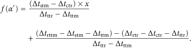$\alpha \prime$ , with constant values for $\mathrm{\Delta }{t}_{\text{xxx}}$ as defined by means of experimentation for the five given queries, results in the function detailed below. It expresses the value of $\beta \prime$ in function of $\alpha \prime$ where scheduling the reasoning on the remote node is equally expensive in terms of power consumption, compared to the situation where the reasoning is scheduled on the back-end,

$\begin{array}{cc}\hfill f\left(\alpha \prime \right)& =\frac{(\Delta t_{\text{stm}}-\Delta t_{\text{ctr}})\times x}{\Delta t_{\text{ttr}}-\Delta t_{\text{ttm}}}\hfill \\ \hfill & \hspace{1em}+\frac{(\Delta t_{\text{rttm}}-\Delta t_{\text{stm}}-\Delta t_{\text{ttm}})-(\Delta t_{\text{rtr}}-\Delta t_{\text{ctr}}-\Delta t_{\text{ttr}})}{\Delta t_{\text{ttr}}-\Delta t_{\text{ttm}}}.\hfill \end{array}$

(4)

The above function now expresses the additional power consumption for computation and transmission, compared to idling. Therefore, we can assume that only values ${\alpha }^{\prime }\ge 1$ and ${\beta }^{\prime }\ge 1$ should be considered. The usage of the networking interface or the processor should not result in a decrease of overall power consumption compared to the situation where either devices or components are not used. In Figures 13(a) and 13(b), the graphs represent the situation where both power consumption, that is, remote or back-end reasoning, consume the same amount of power on the remote constrained node. Each of the plotted lines indicates the situation for one of the five queries, as used in the previous evaluation and presented in Section 6.1. Based on the values obtained during the experiments, we have substituted the remaining variables with concrete values. These values were obtained during the evaluation of the MTSS, MTSSc, and MTSSdc algorithms. For each query, the middle thirty executions of that query were considered and averaged. The conversion table, indicating these values for each of the variables, can be found in Table 6. In the names of the queries the suffix of rs denotes the result set size and the suffix of tp details the number of query triple patterns to be matched.

Table 6

Overview of the actual values for the remaining variables in each of the five evaluated queries.

	$\mathrm{\Delta }{t}_{\text{rttm}}$	$\mathrm{\Delta }{t}_{\text{stm}}$	$\mathrm{\Delta }{t}_{\text{ttm}}$	$\mathrm{\Delta }{t}_{\text{rttr}}$	$\mathrm{\Delta }{t}_{\text{ctr}}$	$\mathrm{\Delta }{t}_{\text{ttr}}$
q_rs44tp1	5,181 ms	215 ms	4,194.5 ms	1,773.81 ms	610.04 ms	417.02 ms
q_rs2166tp5	5,181 ms	215 ms	4,194.5 ms	8,364.67 ms	3,446 ms	833.33 ms
q_rs8100tp7	5,181 ms	215 ms	4,194.5 ms	11,163.67 ms	5,777.67 ms	1,197.33 ms
q_rs11664tp8	5,181 ms	215 ms	4,194.5 ms	17,608.5 ms	9,146 ms	2,254 ms
q_rs48384tp9	5,181 ms	215 ms	4,194.5 ms	59,544 ms	3,412.9 ms	11,478 ms

Figure 13

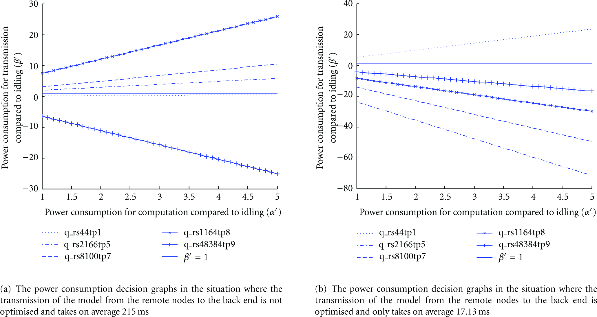
The graphs indicate the situation where the power consumption for reasoning on the remote node is equal to the power consumption for reasoning on the back end. The tuples ( ${\alpha }^{\prime },{\beta }^{\prime }$ ) in the area above the graphs favour a remote reasoning scheduling, the tuples in the area below favour reasoning on the back end. The tuples represent the fraction of the computation power consumption compared to the power consumption when idling ( ${\alpha }^{\prime }$ ), and the fraction of the transmission power consumption compared to the power consumption when idling ( ${\beta }^{\prime }$ ).

Based on the graphs in Figure 13(a) and the fact that we only consider the situation where ${\alpha }^{\prime }\ge 1$ and ${\beta }^{\prime }\ge 1$ , we can conclude that for query q_rs2166tp5, query q_rs8100tp7 and query q_rs11664tp8 the scheduling option of remote reasoning can be beneficial in terms of the power consumption, in the case the power consumption for transmission (NIC) is a few times more than the power consumption for reasoning (CPU). The reason for this is to be found in a positive balance between, on the one hand, the time needed for reasoning and the time needed to transfer the result set on the other hand. The fact that query q_rs44tp1 rarely qualifies ( ${\alpha }^{\prime }/{\beta }^{\prime }=0.1$ ) for back-end reasoning is because it is a relative simple query, with only one triple pattern to be matched and only a limited amount of results, namely, 44 individuals. Query q_rs48384tp9 never favours a remote reasoning scheduling option, because the size of its serialised result set is larger than the size of the serialised ontology model. In the case when caching strategies and model differences transmission are taken into account, one can clearly conclude that the power consumption for transmission reduces significantly. This results in the graphs illustrated in Figure 13(b), where only query q_rs44tp1 still potentially qualifies for the remote reasoning scheduling option.

6.5. Performance Evaluation: Summary

The evaluation presented in this section has shown the advantages of intelligent distribution of DL-Reasoning tasks on the nodes in a network. We started by taking an adaptive approach—the MTSS, MTSSc and MTSSdc algorithms—using a 1st order IIR filter modified average on bandwidth utilisation to decide which scheduling option consumes the least amount of traffic. We have shown that a great improvement can be achieved by combining compression mechanisms with the transmission of differences in the remote ontology model. A viable alternative to the 1st order IIR filter modified average approach has been demonstrated by means of the RSSE algorithm, which can estimate the size of the result set for a given query and general model characteristics on the condition that the query does not combine a selective nature with a large amount of variables. Finally, we have theoretically analysed the OPC algorithm for the situation of five illustrative queries with increasing complexity. We can conclude that power optimisation strategies can be beneficial for these DL-Reasoning tasks when the hardware involved differentiates sufficiently between the power consumed during idle state, reasoning, and transmission.

7. Conclusions and Future Work

In this paper we have described the results of our research and developments into a supporting distributed DL-Reasoning platform, enabling optimised context-aware scheduling of DL-Reasoning tasks. A number of use cases were identified in the scope of context-aware city services. This was followed by an introduction to ontologies and description logics reasoning, together with an overview of related work in the area of semantic web technologies and wireless sensor networks. The main contribution of this paper contains the presentation of the developed distributed reasoning platform, enabling the adoption of ontology-based information processing within the constrained nature of wireless sensor network. Specific optimisation algorithms to minimise the bandwidth utilisation between the WSN and the back end, namely, the MTSS, MTSSc, MTSSdc and RSSE and minimise the power consumption of the nodes in the WSN, that is, the OPC algorithm, were detailed. The presented algorithms were subsequently thoroughly evaluated on the real-life testbed WiLab.t.

The first research question solved by our approach is to bring wireless sensor and mesh networks together with ontology-based methodologies and this in a context-aware environment. To reach this goal, we defined a number of representative use cases and used these to design the supporting DL-Reasoning platform. Secondly, we have implemented the necessary scheduling approaches to technically prove the collaboration of data processing and information classification in a distributed setting, taking into account as much localised information as possible. Lastly, we wanted to optimise the workflow of the platform. Therefore, to formulate an answer on the third and main research question, the adoption of bandwidth optimisation strategies has resulted in significant savings in bandwidth utilisation of 69.48% for the MTSSc algorithm and 92.89% for the MTSSdc algorithm, compared to the MTSS algorithm, without sacrificing any platform functionality. However, because of the specific nature of DL-Reasoning tasks and the characteristics of the hardware, special attention needs to be given when to offload reasoning tasks for specific queries to remote nodes in the context of power optimisation strategies (OPC algorithm). The reason for this has to be found in the potential imbalance between the time needed to compute the results of the description logics model and the time needed to transfer the result set towards the front-end user application. Using our result set size estimation algorithm (RSSE), the bandwidth utilisation optimisation algorithms can also proactively choose the option consuming the least amount of bandwidth, even in the case when for a particular model and query no historical data is available and reactive scheduling is therefore not possible. We have proven by means of an established benchmark that a correct estimation is performed in 11 of the 14 queries. This results in an acceptable estimation for most of the queries in a context-aware setting, except for those queries with many variables and a very restrictive nature. Should such queries be offered to the system regularly, either the 1st order IIR filter modified average mechanism will automatically correct this or the constraints in the query should be included in the ontology model itself.

Future work consists of developing an automatic conversion algorithm for such complex and restrictive queries and to adapt the ontology models at runtime. This should reduce the number of queries in which the RSSE algorithm overestimates the size of the result set. A potential approach could be to extract the individual query triple patterns and to include a new concept in the ontology, defined by means of existential quantification, representing this extracted query triple pattern. Additionally, we plan to study how we can extend the current architecture towards a platform in which underlying remote nodes can again delegate incoming DL-Reasoning tasks to other nodes in the network.