Sage Journals: Discover world-class research

Abstract

Determining the physical positions of sensors has been a fundamental and crucial problem in wireless sensor networks (WSNs). Due to the inherent characteristics of WSNs, extremely limited resources available at each low-cost and tiny sensor node, connectivity-based range-free solutions could be a better choice to feature a low overall system cost. However, localization by means of mere connectivity may underutilize the proximity information available from neighborhood sensing. Although received signal strength (RSS) values are irregular and highly dynamic, it might provide heuristic information about which neighboring nodes are closer and which are further. We propose a distributed Mobile-beacon-assisted localization scheme based on RSS and Connectivity observations (MRC) with a specific trajectory in static WSNs. To ensure that MRC performs as true to reality as possible, we propose two improved approaches based on MRC to consider irregular radio scenario in the noisy environment. Comparing the performance with three typical range-free localization methods in static WSNs, our lightweight MRC algorithm with limited computation and storage overhead is more suitable for very low-computing power sensor nodes that can efficiently outperform better with only basic arithmetic operations in the simulation and physical environments.

1. Introduction

Wireless sensor networks (WSNs) have gained worldwide attention in recent years, particularly with the proliferation in micro-electro-mechanical systems (MEMSs) technology which has facilitated the development of smart sensors [1]. Determining the physical positions of sensors has been a fundamental and crucial problem in WSNs; for example, numerous location-dependent applications with sensor networks are proposed, such as habitat monitoring, battle-field surveillance, and enemy tracking. In addition, some of the routing protocols and network management mechanisms proposed for such networks are built on the assumption that geographic parameters of each sensor node are available [2].

Several schemes have been proposed for dealing with the sensor node localization. Based on whether accurate ranging is conducted at resource-constrained sensor node, the current approaches mainly fall into two categories: range-based and range-free. First, range-based approaches assume that sensor nodes are able to measure the distances, or even relative directions of their neighbor nodes, based on time of arrival (TOA), time difference of arrival (TDOA), angle of arrival (AOA), and received signal strength (RSS) technologies, and so forth. The range-based schemes typically have higher location accuracy but require additional hardware to measure distances or angles. Second, range-free approaches localize sensor nodes based on simple sensing, such as anchor proximity, connectivity-based, or localization events detection. Although the range-free schemes accomplish as high precision as the range-based ones, they provide an economic approach.

Due to the inherent characteristics of WSNs, extremely limited resources available at each low cost and tiny sensor node, connectivity-based solutions in range-free approaches could be a better choice to feature a low overall system cost. However, localization by means of mere connectivity may underutilize the proximity information available from neighborhood sensing [2]. A popular and widely used neighborhood sensing technique, always available in many sensor platforms such as Mica2, MicaZ, and TelosB, is RSS which is usually used in the range-based localization. Although RSS values are irregular and highly dynamic, the difference in RSS values consistently reflect the contrast of physical distances [3]; that is, RSS might provide heuristic information about which neighboring nodes are closer and which are further [2].

The experiment results [2] have confirmed that network-wide monotonic relationship between RSS and physical distance does not hold. For example, at the receiver side, RSS sensing results are sensitive to small variance among different nodes [2]. However, the experiment results [2] have also confirmed that the monotonic RSS-distance relationship holds much well in the case of one sensor node. In addition, using a single mobile beacon that knows its position is broadly equivalent to using many static anchors each broadcasting once. These two facts motivate us to believe that a single mobile beacon which can travel the entire deployment region based on some traverse route can be used to help localize the entire network by connectivity observations and RSS relationship between the unknown node and the mobile beacon.

In this paper, we propose a distributed Mobile-beacon-assisted localization scheme based on RSS and Connectivity observations (MRC) with a specific trajectory in static WSNs. After the unknown nodes are deployed in a fixed-size area, a mobile beacon traverses the area while broadcasting packets. Then, the unknown nodes continuously observe the connectivity information from the mobile beacon. As a result, the unknown nodes' locations are bounded in the beacon's transmission area. Next, the unknown nodes utilize the comparison result of RSS from any two contacted neighbor beacons to narrow the location region of unknown node. To this end, the accuracy can be further improved when the unknown node obtains more comparison results from the connected beacon positions.

Furthermore, we also propose two improved approaches based on MRC, called MRC_Nearest and MRC_Centroid to consider the irregular radio scenario in the noisy environment. To ensure that MRC performs as true to reality as possible, four possible connectivity scenarios to the unknown node are further considered in the more general radio model. Evaluations show that the MRC_Centroid algorithm is robust and performs well even with severe interference.

This paper offers the following three major contributions:

(i) Improved Connectivity Restriction

we give a mobile beacon's trajectory for MRC in which some remarks regarding necessary properties are considered. Its novelty lies in combining 1-hop and 2-hop beacon position restrictions (connectivity restriction) at the same time;

(ii) Further Neighborhood Sensing Restriction

we utilize the proximity information available from neighborhood sensing as distance-related information (neighborhood sensing restriction) to further improve the precision of connectivity-based range-free localization in the mobile-beacon-assisted pattern;

(iii) Lightweight Computation and Storage

any unknown node only requires lightweight computation to solve the translation of position and limited storage overhead to retain (mainly 3 or 4) RSS and connectivity observations information whether or not the radio model is regular.

Comparing the performance with three typical range-free localization methods, the existing classic range-free localization algorithms with multiple static anchors, a single mobile-beacon-assisted range-free localization algorithm, and RSS-assisted range-free localization in static WSNs, our lightweight MRC algorithm with limited computation and storage overhead is more suitable for very low-computing power sensor nodes that can efficiently perform only basic arithmetic operations. Evaluation results show that MRC outperforms better in the simulation and physical environments.

The rest of this paper is organized as follows: Section 2 gives an overview of related works. Section 3 presents details of the proposed MRC, MRC_Nearest, and MRC_Centroid algorithms. Sections 4 and 5 show and discuss the simulation and physical evaluation results, respectively. Finally, Section 6 concludes our works.

2. Related Works

There has been a significant research activity in the area sensor network localization. Based on whether the range measurements are used at the resource-constrained sensor nodes, most of the existing approaches about sensor node localization fall into two categories: (1) range-based and (2) range-free localization. In addition, the sensor networks already incorporate GPS-equipped mobile beacon as part of the design, which can be a cost-effective way of achieving sensor node localization. In this section, we provide a brief literature review of these localization approaches.

Range-based approaches compute per-node location information iteratively or recursively based on measured distances among unknown nodes and a few anchors which precisely know their locations. Many range-based methods use techniques such as TOA [4, 5], TDOA (e.g., Cricket [6], AHLos [7], TPS [8]), AOA (e.g., APS [9], SpinLoc [10]), and RSS (e.g., Radar [11], wMDS [12], IndoorGPS [13], Sequence [14], Ranking [15]) to measure distance or angles among unknown nodes and anchors. Although range-based solutions can be suitably used in small-scale indoor environments, they are considered less cost effective for large-scale deployments.

Range-free approaches do not require accurate distance measurements but localize the unknown node based on anchor proximity (e.g., Centroid [16], APIT [17]), network connectivity information (e.g., DV-hop [18], MDS-MAP [19], SDP [20]), or localization events detection (e.g., Lighthouse [21], Spotlight [22]). Recently, some RSS-assisted range-free approaches are proposed, such as RSSL [23], PI [3], and RSD [2]. Instead of using absolute RSS to estimate the distance between two nodes with ordinary hardware, by contrasting the measured RSS values from the mobile beacon to a sensor node, RSSL and PI utilize the variance of RSS to estimate the unknown node position. Observing that per-node monotonic RSS-distance relationship holds well, RSD captures a relative distance between 1-hop neighboring nodes from their neighborhood orderings to achieve better positioning accuracy than connectivity alone. For range-free connectivity-based localizations such as MDS-MAP and DV-hop, applying RSD is easy. Inspired by the empirical data results “Network-wide monotonic relationship between RSS and physical distance does not hold, but per-node monotonic RSS-Distance relationship holds well” shown in the RSD methods, but we propose a totally different range-free localization solution.

In addition, much research has been done on mobile-beacon-assisted localization for WSNs. The mobile beacon travels through the deployment area while broadcasting its location along the way. Unknown nodes localize themselves by monitoring range or connectivity information coming from the beacon. A general survey about mobile-beacon-assisted approaches can be found in [24]. Here, we review some works closely related to our proposed algorithms.

The paper [25] proposed some static paths to guide the GPS-equipped mobile beacon to achieve better coverage, better accuracy, and shorter path length, which is consistent with our design goals of trajectory. Significantly different from these static paths which are designed for range-based sensor network localization, such as RSS, TOA, and AOA under most common noise models (mostly Gaussian), our trajectory is designed for one of range-free approaches, based on RSS and connectivity observation.

In the range-free, distributed, and probabilistic algorithms MSL [26] and MSL*, each sensor node uses observations from only those neighbors (1-hop) that have better location estimates than it; that is, the weight of a sample is determined using the neighbors' observations besides the location announcements from the beacons. MSL modified the mobility model to allow this algorithm to work in static WSNs. MBL [24] relies on direct arriver and leaver information (2-hops) from a single mobile-assisted beacon which outperforms MSL when both of them use only a single mobile beacon with random trajectory for localization in static WSNs. All of these methods (MSL, MBL, and their improved versions) use the particle filter [27] (also called sequential Monte Carlo method) to perform a probabilistic localization on a sample representation. However, particle filters approach is quite power consuming in the tiny sensor nodes.

Our proposed methods differ significantly from those previous mobile-beacon-assisted range-free localization works because we utilize a mobile beacon with a specific trajectory and observe both the neighborhood sensing and connectivity observations (1-hop and 2-hop restrictions) with lightweight computation and storage overhead to improve precision in the localization process.

3. Design

3.1. MRC Localization Scheme

In this section, we describe our novel Mobile-beacon-assisted localization based on RSS and Connectivity observations, which we call MRC. Let us consider a sensor network with M static sensor nodes in a 2D plane which do not have a priori known locations (called unknown nodes) and a single mobile node (called beacon or anchor), equipped with localization hardware, for example, GPS, which allows it to know its location at all times. Here, we suppose that each sensor (unknown node or beacon) has the same ideal radio range r. In the regular radio model, the transmission range is equal to radio range, and, in the irregular radio model, the transmission range will be influenced by the environment noise. Any two sensors are called neighbors (or neighborhood) if the distance between them is less than or equal to the one-hop transmission range, otherwise known as unneighbor. After random deployment of the unknown nodes in a fixed-size area, the beacon traverses the entire sensor network with a specific trajectory while broadcasting packets which contain the coordinates of its own and some other related information. At any time, every unknown node within the radio range of the mobile beacon will hear a location announcement (called connectivity observation) from that beacon. We do not assume very tightly synchronized clocks. In a realistic deployment, it would be necessary to deal with network collisions and account for missed messages [28]. Location estimates and observations are assumed to be available at discrete times. For dynamic state estimation, the discrete-time approach is widespread and convenient [27].

Any unknown node receiving the packets from the mobile beacon can recognize that it is in the area around the beacon's current location with a certain probability. With each connectivity observation in a series of different times, the unknown node's location is bounded in the beacon's transmission area. The accuracy can be improved when the unknown node obtains more connectivity observations from the beacon. In addition, the unknown node further obtains the geometrical relationship of a series of beacon positions by contrasting the measured power of the signal at the receiver. Namely, after adopting the connectivity observation, the unknown node utilizes the comparison result of RSS derived from any two neighbor beacon positions to narrow the estimated location region of unknown node. As a result, the precision of position can be improved when the unknown node obtains more comparison results from the neighbor beacons.

Figure 1 shows an example situation. We supposed that the point A, B, and C shown in Figure 1 is a series of positions of mobile beacon passed. The unknown node could derive nonneighbor beacon positions by its neighbor beacon positions. This assumption will hold as long as the unknown node obtains the trajectory of mobile beacon. Thus, the unknown node S knows the beacon position A, B, and C in Figure 1. The unknown node S obtains the connectivity observation from the beacon positions A and B and does not receive the packets from the beacon position C. Then, the unknown node knows it is within distance r of beacon positions A and B but must not be located within the distance r of beacon position C; that is, the position of the unknown node S is within the shaded region in Figure 1. Next, the unknown node S compares the RSS values obtained from beacon positions A and B. The comparison result shows that the RSS value obtained from position A is larger than B, $S A > S B$ ; that is, the beacon position A is closer than the beacon position B from the unknown node position S, $| A S | < | B S |$ , where SA and SB denote the corresponding RSS values and $| A S |$ and $| B S |$ denote the corresponding distances. It is straightforward to show that the red-shaded region in Figure 1 enumerates all the possible estimated locations of the unknown node S.

Figure 1

MRC localization scheme.

If the measured two RSSs are the same or very close, that is, the difference between these two RSS values is less than a threshold, then the unknown node takes the center of these two beacon positions as its estimated position.

3.2. Trajectory of Mobile Beacon

The mobile-assisted localization scheme faces a new problem, “What is the optimum beacon route (as the same concept trajectory in our paper, beacon trajectory in [29], movement strategy in [30], movement pattern in [23], and movement path in [31])?” [29] or called trajectory selection problem. Notice that the problem is quite difficult. On one hand, the position of the unknown node is not known a priori [29]. Then, the trajectory of mobile beacon cannot be designed for the specific distribution of unknown nodes in the deployment area. On the other hand, the movement strategy of mobile beacon should be related to the specific localization scheme. Namely, the optimum trajectory in one mobile-beacon-assisted localization scheme is not necessarily optimal in the others. To this end, the trajectory of the mobile beacon to locate all the unknown nodes needs further considerations.

In this section, we will make some remarks regarding the following characteristics that the trajectory for MRC should have.

First, to improve the average position accuracy of unknown nodes, the trajectory of mobile beacon should cover the entire unknown nodes deployment area; that is, all the unknown nodes should be located when the mobile beacon completes all the paths.

Second, due to the limited resources available in the tiny sensor nodes, the trajectory of mobile beacon should be shorter, so as to achieve shorter location time and consume smaller energy cost. In addition, the unknown node should derive the unneighbor beacon position from such limited number of known neighbor beacon positions, easily, to further narrow the bounded transmission area obtained from neighbors' connectivity observation.

Third, the accuracy can be further improved when the unknown node contacts more neighbor beacons. However, the computational complexity of the unknown node also increases. Thus, the trajectory of mobile beacon should obtain a tradeoff between the localization accuracy and the computational complexity.

Therefore, let us consider the above characteristics to give the following trajectory of the mobile beacon shown in Figure 2, in which red-dotted line denotes the trajectory of mobile beacon. Figure 2 shows the length L and the width W of rectangular sensor nodes deployment area. The mobile beacon moves along the direction of the arrow in the red-dotted line, and the small circles denote a series of beacon positions. Namely, the mobile beacon starts from position A, through B, C two positions, to position D, then continues moving along the red-dotted line, and finally to position E. The distance between any two adjacent beacon positions of movement is r; that is, the minimum distance between the transmitted beacon points is equal to the radio range. This configuration of distance can obtain a tradeoff between the localization accuracy and the length of trajectory as shown in the latter evaluations. The arc in Figure 2 denotes the radio range of the corresponding beacon position.

Figure 2

Trajectory of mobile beacon.

This movement pattern for MRC meets the previously mentioned remarks. First, the rectangle area in Figure 2 represents the largest possible area of unknown node deployment. Any unknown node in this area can contact the connectivity information from the beacon 3 or 4 times; that is, all possible positions of unknown nodes are fully covered by at least 3 or 4 noncollinear beacons. Second, trajectory length is much smaller than the random trajectory in MBL and is very close to some classic trajectory, such as movement pattern in ADO [23], optimal trajectory in PI [3]. In addition, the unknown node could judge the unneighbor beacon' positions from these 3 or 4 contacted neighbor beacons's position, and these unneighbor beacon positions could be used as 2-hop noncontacted position information. Third, the localization precision of MRC with this movement pattern is much higher as shown in latter evaluations. In addition, each unknown node only observes 3 or 4 times connectivity information and compares limited RSS values.

3.3. Regular Radio Model

The MRC algorithm can be broken down into three stages: (1) beacon acquisition, (2) region determination, and (3) location calculation. These stages are performed at individual unknown node in a purely distributed fashion.

(1) Beacon Acquisition

In the first stage, the mobile beacon is traversing the specified location in the unknown node deployment area as the trajectory described in Section 3.2. At each specified position, the mobile beacon broadcasts packets which contain the coordinates of its own and some other related information. When the unknown node itself is within the radio range of the mobile beacon's current specified position, the unknown node will obtain the connectivity observations from the beacon and measure the corresponding RSS values. The unknown node retains this information in the memory until the end of localization.

(2) Region Determination

When the mobile beacon with the trajectory finishes moving, any unknown node will contact the mobile beacon three, four, or six times in the rectangular deployment area. Without loss of generality, we show the first two cases in Figure 3.

Figure 3

Different location regions.

Case 1 (3-connectivity).

If the unknown node only contacts 3 times with the mobile beacon throughout mobile beacon moving process, the position of unknown node is within the overlapping regions of the transmission area of these three contacted mobile beacon positions and out of any other radio range of beacon positions. We call this case of relationship between the unknown node and beacon positions 3-connectivity.

As shown in Figure 3, the unknown node S is in the radio range of beacon positions A, B, and C and out of any other beacon positions, such as D, E, and F. Then, the unknown node is within the area formed by Region (1)~Region (6) shown in Figure 3. The advantage of 3-connectivity case to unknown node is the ability to combine 1-hop and 2-hop beacon position restrictions at the same time; that is, the unknown node with 3-connectivity case is within 1-hop neighbor beacon positions (A, B, and C) and out of 2-hop beacon positions (D, E, and F).

Once the 3-connectivity case happens, the RSS values from these three beacon positions A, B, and C in the unknown node have been measured, and the unknown node obtains the value SA, SB, and SC, respectively.

If $S A < S B$ and $S A < S C$ and $S B < S C$ , then the unknown node S is within the Region (1).

If $S A > S B$ and $S A < S C$ and $S B < S C$ , then the unknown node S is within the Region (2).

If $S A > S B$ and $S A > S C$ and $S B < S C$ , then the unknown node S is within the Region (3).

If $S A > S B$ and $S A > S C$ and $S B > S C$ , then the unknown node S is within the Region (4).

If $S A < S B$ and $S A > S C$ and $S B > S C$ , then the unknown node S is within the Region (5).

If $S A < S B$ and $S A < S C$ and $S B > S C$ , then the unknown node S is within the Region (6).

Thus, after adopting the 3-connectivity observation with 1-hop and 2-hop restrictions, the unknown node utilizes the comparison result of RSS to further narrow the estimated location region of unknown node.

Case 2 (4-connectivity).

If the unknown node just contacts 4 times with mobile beacon throughout mobile beacon moving process, the position of unknown node is within the overlapping regions of the transmission area of these four contacted mobile beacon positions and out of any other radio range of beacon positions. We call this case of relationship between the unknown node and beacon positions 4-connectivity.

As shown in Figure 3, the unknown node S is within one of 4 beacon positions (e.g., ABCD, ABCE, or ABCF) transmission area, and out of any other beacon positions. Without loss of generality, let the unknown node be within the radio range of beacon positions A, B, C, and D. Then, the unknown node is within the area formed by Region (7)~Region (10).

Once the 4-connectivity case happens, the RSS values from four beacon positions A, B, C, and D in the unknown node have been measured, and the unknown node obtains the value SA, SB, SC, and SD, respectively.

If $S A > S D$ and $S B < S C$ , then the unknown node S is within the region (7).

If $S A > S D$ and $S B > S C$ , then the unknown node S is within the region (8).

If $S A < S D$ and $S B > S C$ , then the unknown node S is within the region (9).

If $S A < S D$ and $S B < S C$ , then the unknown node S is within the region (10).

Case 3 (7-connectivity).

If the unknown node S receives seven different beacon positions connectivity information, then S is on the trajectory of the mobile beacon. This special case is called 7-connectivity. It is obvious that S is uniquely determined by such seven beacon positions. S will take the centroid of seven connected beacon positions as its position.

(3) Location Calculation

After the position of unknown node is restricted to a particular region in the previous stage, the unknown node will take the centroid of restricted region as its estimated position.

Case 1 (3-connectivity).

The triangle formed by three beacon positions in the 3-connectivity case is either Upper triangle or Lower triangle, where Upper triangle denotes the x-coordinate of one beacon position larger than the other two beacon positions' x-coordinate. As shown in Figure 4, the triangles $A B C$ and $B D C$ belong to Upper triangle and Lower triangle, respectively. We denote different restricted region by U.1~U.6 in the Upper triangle and L.1~L.6 in the Lower triangle. If we can obtain the centroid of region U.1 in Figure 4, any other centroid of region in the Upper and Lower triangles will be determined by the geometrical symmetry.

Now, we calculate the centroid of restricted region $U . 1$ . We denote the horizontal x and vertical y of region U.1 centroid u1 by $u 1 = (u 1 \cdot x, u 1 \cdot y)$ . As shown in Figure 4, we assume that the midpoint of line segment $B C$ is located in the origin of coordinate O and $| B C | = r$ . From the definition of centroid, the geometric center of the object's shape, we obtain

\begin{gathered} u 1 \cdot x = \frac{\int_{0}^{r / 2} \int_{\sqrt{r^{2} - x^{2}} - (\sqrt{3} / 2) r}^{- (\sqrt{3} / 3) x + (\sqrt{3} / 6) r} x d y d x}{\int_{0}^{r / 2} \int_{\sqrt{r^{2} - x^{2}} - (\sqrt{3} / 2) r}^{- (\sqrt{3} / 3) x + (\sqrt{3} / 6) r} d y d x}, \\ u 1 \cdot x = \frac{\int_{0}^{r / 2} \int_{\sqrt{r^{2} - x^{2}} - (\sqrt{3} / 2) r}^{- (\sqrt{3} / 3) x + (\sqrt{3} / 6) r} y d y d x}{\int_{0}^{r / 2} \int_{\sqrt{r^{2} - x^{2}} - (\sqrt{3} / 2) r}^{- (\sqrt{3} / 3) x + (\sqrt{3} / 6) r} d y d x} . \end{gathered}

(1)

Figure 4 shows that $u 2$ and $u 1$ are two centroid points which are symmetric with respect to a given line segment $C E$ . The equation of the line through points C and E is given by

(2 \sqrt{3}) x + 6 y - \sqrt{3} r = 0 .

(2)

Thus,

\begin{gathered} u 2  \cdot  x  =  u 1  \cdot  x  -  \frac{2  *  (2 \sqrt{3})  *  ((2 \sqrt{3})  *  u 1  \cdot  x  +  6  *  u 1  \cdot  y  -  \sqrt{3} r)}{\sqrt{({(2 \sqrt{3})}^{2}  +  6^{2})}}, \\  u 2  \cdot  y  =  u 1  \cdot  y  -  \frac{2  *  6  *  ((2 \sqrt{3})  *  u 1  \cdot  x  +  6  *  u 1  \cdot  y  -  \sqrt{3} r)}{\sqrt{({(2 \sqrt{3})}^{2}  +  6^{2})}} , \end{gathered}

(3)

u 3

and

u 2

are two centroid points which are symmetric with respect to a given line segment

B F

. The equation of the line through points B and F is given by

(2 \sqrt{3}) x - 6 y + \sqrt{3} r = 0 .

(4)

Thus,

\begin{gathered}  u 3  \cdot  x  =  u 2  \cdot  x  -  \frac{2  *  (2 \sqrt{3})  *  ((2 \sqrt{3})  *  u 2  \cdot  x  -  6  *  u 2  \cdot  y  +  \sqrt{3} r)}{\sqrt{({(2 \sqrt{3})}^{2}  +  6^{2})}} , \\  u 3  \cdot  y  =  u 2  \cdot  y  -  \frac{2  *  6  *  ((2 \sqrt{3})  *  u 2  \cdot  x  -  6  *  u 2  \cdot  y  +  \sqrt{3} r)}{\sqrt{({(2 \sqrt{3})}^{2}  +  6^{2})}} , \end{gathered}

(5)

u 4

and

u 3

u 5

and

u 2

u 6

and

u 1

, these centroid points are symmetric with respect to y-axis, respectively.

Thus,

\begin{gathered} u 4 \cdot x = - u 3 \cdot x, u 4 \cdot y = u 3 \cdot y, \\ u 5 \cdot x = - u 2 \cdot x, u 5 \cdot y = u 2 \cdot y, \\ u 6 \cdot x = - u 1 \cdot x, u 6 \cdot y = u 1 \cdot y . \end{gathered}

(6)

The Lower triangle $B D C$ and Upper triangle $A B C$ are symmetric with respect to x-axis. The centroid of region in the Lower triangle can be obtained by the symmetric centroid in the Upper triangle.

Figure 4

Relative regions.

Case 2 (4-connectivity).

Any four points in 4-connectivity case form two equilateral triangles, where one is Upper triangle, and the other is Lower triangle, for example, equilateral Upper triangle $A B C$ and Lower triangle $B D C$ in $A B D C$ 4-connectivity case of Figure 3. Without loss of generality, the Regions (11), (12), (15), and (16) in Figure 3 are in the Upper triangle, and the Regions (9), (10), (13), (14), (17), and (18) in Figure 3 are in the Lower triangle. We denote different restricted region in 4-connectivity case by U.7~U.12 in the Upper triangle and L.7~L.12 in the Lower triangle in Figure 4. If we can obtain the centroid of region $U . 7$ in Figure 4, any other centroid of region will be determined by the geometrical symmetry.

The centroid of region $U . 7$ denoted as $u 7$ is obtained by

\begin{gathered} u 7 \cdot x = \frac{\int_{0}^{r / 2} \int_{0}^{\sqrt{r^{2} - x^{2}} - (\sqrt{3} / 2) r} x d y d x}{\int_{0}^{r / 2} \int_{0}^{\sqrt{r^{2} - x^{2}} - (\sqrt{3} / 2) r} d y d x}, \\ u 7 \cdot y = \frac{\int_{0}^{r / 2} \int_{0}^{\sqrt{r^{2} - x^{2}} - (\sqrt{3} / 2) r} y d y d x}{\int_{0}^{r / 2} \int_{0}^{\sqrt{r^{2} - x^{2}} - (\sqrt{3} / 2) r} d y d x} . \end{gathered}

(7)

Similar to the symmetric centroids obtained in 3-connecivity case, other centroids in 4-connectiviy case can be obtained easily.

Once we obtain the relative centroid of different restricted regions in Figure 4, any unknown node estimated absolute position will be calculated by coordinate shift. For example, we suppose that an unknown node q only contacts the mobile beacon three times. The three beacon positions are ( $p 1 \cdot x, p 1 \cdot y$ ), ( $p 2 \cdot x, p 2 \cdot y$ ), and ( $p 3 \cdot x, p 3 \cdot y$ ), where $p 1 \cdot x > p 2 \cdot x$ ; namely, these three beacon positions form an Upper triangle. If the relative position of unknown node belongs to Region $U . 1$ in the Upper triangle, the estimated position q is calculated by

(q \cdot x, q \cdot y) = (u 1 \cdot x + p 1 \cdot x, u 1 \cdot y + p 1 \cdot y - (\frac{\sqrt{3}}{2}) r) .

(8)

To avoid the integral operation of centroid calculation in the unknown node, the beacon transmits the calculated relative coordinates about $u 1$ and $u 7$ with specified radio range when contacting the unknown node for the first time. Then, any other centroid of region will be determined by the geometrical symmetry.

As described above, any unknown node only retains a limited number of RSS values (mainly 3 or 4) in the memory and requires simple arithmetic to solve the translation of position. Namely, MRC is a lightweight localization approach.

3.4. Irregular Radio Model

Our previously proposed localization approach MRC assumes an ideal radio scenario, where location sensory data are not influenced by the irregular radio range; that is, any receiver within the radio range of sender will hear the packets from that sender. However, on the one hand, variability in actual radio transmission patterns can have a substantial impact on localization accuracy depending on the localization technique [28]. On the other hand, the packet reception depends not only on the sender but also on the receiver. To this end, a perfect circular radio model assumption on real testbeds could be invalid for WSNs.

In this section, to ensure that MRC performs as true to reality as possible, we use a more general radio model [17] in our assumption. As the model described in [17], we assume an irregular radio transmission model with an upper and lower bounds on signal propagation. Namely, beyond the upper bound, all are out of communication range. Within the lower bound, every sensor node is guaranteed to be within communication range.

If the radio range is between these two boundaries, four scenarios are possible: (1) less than or equal to 2-connectivity, (2) 3-connectivity, (3) 4-connectivity, and (4) greater than or equal to 5-connecitvity.

Case 1 (less than or equal to 2-connectivity).

If the radio transmission suffers severe interference effects from environmental noise, the unknown node may hear the connectivity observation only 1 or 2 times from the mobile beacon. As shown in Figures 5(a) and 5(b), the unknown node observes the connectivity from the beacon position in the solid black dot and does not hear from hollow black spot.

Figure 6 shows 1-connectivity case; the unknown node is out of any other beacon positions' radio range, such as A, B, C, D, E, and F, but within the radio range of the beacon position O. Then, the possible location of the unknown node is within the nonshadow coverage area, that is, near the beacon position O in Figure 6. Thus, the unknown node takes the only contacted beacon location O as its estimated location.

Figure 5

Connectivity of different cases.

Figure 6

Connectivity with noise.

Case 2 (3-connectivity).

Figures 5(c), 5(d), and 5(e) show all possible mutual position scenarios of three different beacon positions, respectively: (1) equilateral triangle, (2) isosceles triangle, and (3) collinear.

To distinguish three kinds of scenarios, the unknown node calculates the distance between any two beacon positions. Then, it calculates the number of those distances equal to the radio range. If the number is equal to three, the unknown node is within the equilateral triangle formed by three different beacon positions. We call this equilateral triangle form case regular 3-connectivity. If the number is equal to two, the node is within the isosceles triangle or near the line segment (collinear). We call these cases irregular 3-connectivity.

Case 3 (4-connectivity).

Figures 5(f) and 5(g) show all possible mutual position scenarios of four different beacon positions: (1) diamond, and (2) nondiamond.

To distinguish these two kinds of scenarios, the node calculates the distance between any two connectivity positions. Then, it calculates the number of those distances equal to the radio range. If the number is equal to five, it shows that the unknown node is within the diamond formed by four different beacon positions. We call this diamond form case regular 4-connectivity. If the number is equal to three, we call the nondiamond form case irregular 4-connectivity.

Case 4 (greater than or equal to 5-connecitvity).

As shown in Figures 5(h) and 5(i), the unknown node hears the beacon connectivity information greater than or equal to five times from the mobile beacon.

In general, these four scenarios can be divided into two types, regular connectivity and irregular connectivity. In the regular connectivity case, that is, regular 3-connectivity and regular 4-connecitvity, the unknown node will adopt 3-connectivity or 4-connectivity algorithm of MRC, respectively. While for the other case, that is, less than or equal to 2-connectivity, irregular 3-connectivity and 4-connectivity and greater than or equal to 5-connecitvity, we propose the following two solutions. (i)

The unknown node compares the RSS values obtained from those contacted beacon positions. Then, the node takes the beacon position making the unknown node receive the largest RSS value from those beacon positions as the estimated location of the node. We call this method MRC_Nearest.

(ii)

From the irregular beacon signals that it receives, the unknown node infers proximity to a collection of reference beacon positions. The unknown node localizes itself to the region which is defined by the centroid of these beacon positions. We call this solution MRC_Centroid.

Different from MRC, MRC_Nearest and MRC_Centroid can perform well in the irregular radio model by dealing with the above different connectivity cases between unknown node and beacon positions. In the evaluation section, we will compare the performance of the two solutions MRC_Nearest and MRC_Centroid in the noise environment.

Finally, let us consider 0-connectivity case; that is, the unknown nodes do not contact any beacon position. In the regular radio model, the mobile beacon with the trajectory will avoid 0-connectivity case. In the irregular radio model, 0-connectivity case is inevitable, but the probability is very small and has little impact on the result of average position accuracy. Once 0-connectivity of some unknown node appears, the unknown node will adopt some localization algorithms (e.g., Centroid localization algorithm) with localized neighbor sensor nodes after the mobile beacon has finished localization.

4. Simulation Evaluation

This section compares the performance with three typical range-free localization approaches closely related to our approaches: (1) classic range-free localization algorithms, (2) connectivity-based mobile-beacon-assisted range-free localization algorithms, and (3) RSS-assisted range-free localization algorithms.

The first type, such as Centroid, DV-hop, APIT, MDS-MAP, and SDP, is mainly designed for a static sensor network with multiple static anchors and unknown nodes. In order to obtain high redundancy of beacons without increasing deployment costs, these methods also can use a single moving anchor that sends out beacons at different locations to localize all unknown nodes inside the sensor network.

The second type, such as MSL and MBL, is specially designed for a static sensor network with a single mobile beacon and static unknown nodes. These mobile-beacon-assisted range-free approaches localize unknown nodes based on connectivity observation only.

The third type, such as PI, RSSL, and RSD, utilizes the variance of RSS to estimate the unknown node position, where the original design goal of PI and RSSL is to work in the mobile-assisted scenario, while RSD can capture the relative distance among 1-hop neighboring nodes to improve performance of the connectivity-base range-free approaches. Thus, RSD could augment some classic range-free localization algorithms, such as DV-hop, called DV-RSD, where the relative distance turns to the smallest accumulated RSD instead of shortest-path hops in DV-hop.

In the following content, assumptions are given in Section 4.1, and compared with three typical localization algorithms, the evaluation results are shown in Sections 4.2, 4.3, and 4.4, respectively.

4.1. Assumption

The key metric [26] for evaluating a localization algorithm is the accuracy of the location estimates or localization error. This is computed as follows:

\begin{gathered} Error = \frac{1}{M} \sum_{i = 1}^{M} ‖ e_{i} - R_{i} ‖, \end{gathered}

(9)

\begin{gathered} M = \frac{n_{d} S}{π r^{2}}, \end{gathered}

(10)

where M is the number of unknown nodes and can be obtained from (10), R_i denotes the real location of the ith unknown node,

e_{i}

denotes the location estimate of the ith unknown node, and

∥ e_{i} - R_{i} ∥

denotes the distance between locations

e_{i}

and

R_{i}

n_{d}

in (10) denotes the unknown node density, the average number of nodes in one-hop transmission range; that is,

n_{d}

is the average number of neighbors to an unknown node. S denotes the size of the deployment area. The errors shown in the simulation results are in terms of the radio range; that is, the errors shown are computed by dividing the error in (9) by the radio range of sensor node.

Most parameter settings for our simulations are those used in [26, 28]. Our results were obtained using sensor nodes randomly distributed in a 500 units × 500 units square field, that is, $S = 500 \times 500$ . In our experiments, we set ideal radio range $r = 100$ , the unknown node density $n_{d} = 10$ . We adopt Walking GPS architecture [32] for the beacon and unknown nodes which significantly reduce the size of the code and data memory used on the sensor node. Other simulation parameters of the unknown node are based on the MicaZ sensor node.

4.2. Compared with Classic Range-Free Localization Approaches

In these experiments, we simulate DV-hop with triangulation procedure to correct the estimated location. We modify APIT so that perfect point-in-triangulation (PIT) test is feasible, because the unknown node within the beacon triangles is easily determined with the trajectory proposed in Section 3.2. We simulate MDS-MAP with classical MDS algorithms. We simulate SDP in Matlab with the generic optimization solver SDPT3, called by CVX [33]. SDPT3 is a state-of-the-art primal-dual interior-point solver that exploits sparsity. Our experimental results are the average of 100 executions with different pseudorandom number generator seeds.

4.2.1. Localization Error When Varying Unknown Node Density

Random Deployment of Beacons

For the classical range-free localization algorithms, the deployment of beacons has no specific way. We put the same number of static anchors as the beacons in the MRC trajectory, randomly deployed in a two-dimensional plane. Due to the small number of random beacons, some unknown nodes will not be restricted by enough beacons. Thus, APIT algorithm is invalid in this case. Figure 7 explores the effect of unknown node density on the localization estimation accuracy. Since, there is no interaction between unknown nodes in Centroid, and MRC algorithms, we see nearly constant results while varying unknown node density. For DV-hop, localization error decreases as the number of neighbors increases. As DV-hop, algorithms MDS-MAP and SDP rely on the observations from the neighbors including the unknown nodes and the beacons, but localization results have little change with different unknown node density. On the whole, our proposed method MRC improves the accuracy of nearly 30%–75% with the specific trajectory of mobile beacon in the perfect circular radio model.

Figure 7

Error varying unknown node density with random deployment of beacons.

Regular Deployment of Beacons

In this experiment, we compare these algorithms under a more consistent condition. Namely, we will deploy the anchors as the trajectory positions of MRC proposed in Section 3.2. Compared with Figure 7, the precision of Centroid and SDP algorithms have been improved nearly 50% due to more uniform anchors deployment, while the precision of DV-hop decreases due to more accurate 1-hop estimation in the random deployment scenario. Compared with the classic range-free localization algorithms with the same anchors positions as the trajectory beacons, the performance advantage of MRC has no significant change in Figure 8.

Figure 8

Error varying unknown node density with regular deployment of beacons.

4.2.2. Localization Error When Varying DOI

We use degree of irregularity (DOI) to denote the maximum radio range variation in the direction of radio propagation. For example, if DOI = 0.1, then the actual radio range in each direction is randomly chosen from [0.9r, 1.1r]. In our experiments, the radio transmission range changes in time. SDP currently does not provide solutions in the noise environment.

Random Deployment of Beacons

As shown in Figure 9, the Centroid and MDS-MAP approaches are not substantially affected when DOI is between 0 and 0.5. The precision of DV-hop, MRC_Nearest, and MRC_Centroid algorithms is decreased as the value of DOI increased. MRC_Centroid method is always better than DV-hop and MRC_Nearest approaches, no matter the change in DOI.

Figure 9

Error varying DOI with random deployment of beacons.

Regular Deployment of Beacons

DV-hop does not work in this case. As shown in Figure 10, the MDS-MAP algorithm is not substantially affected. However, for Centroid, APIT, MRC_Nearest, and MRC_Centroid approaches, localization error increases as well as the value of DOI. Compared to classic range-free localization algorithms when varying DOI from 0 to 0.5, the accuracy of MRC_Centroid outperforms all the other approaches. As a result, in the irregular connectivity case, we conclude that the estimated position of unknown node is defined by the centroid of those contacted beacon positions.

Figure 10

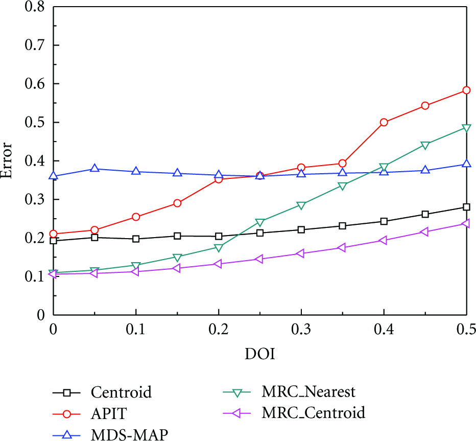
Error varying DOI with regular deployment of beacons.

4.3. Compared with Connectivity-Based Mobile-Beacon-Assisted Range-Free Localization Approaches

In this experiment, we compare MRC algorithms with some connectivity-based mobile-beacon-assisted range-free localization approaches, such as MSL, MBL. In general, as the time goes on, the mobile beacon contacts more unknown nodes; that is, more unknown node will be localized. The average localization accuracy of the mobile-beacon-assisted approaches will continue to be increased. Thus, the comparison of different localization convergences is much important. We simulate MSL and MBL with the number of particles for an unknown node $N = 50$ and adopt our proposed trajectory in Section 3.2 as MRC.

4.3.1. Localization Error As the Time Increased without Noise

Figure 11 shows the comparison of accuracy for MSL, MBL, and MRC under the same trajectory of the mobile beacon with the perfect circular radio model. In general, in all localization approaches, error decreases as the time increases. MSL and MBL utilize the mean of particles as the initial estimated position of unknown node. As shown in Figure 11, MSL and MBL, these two curvatures of the curves are very similar to each other. The results remaining unchanged denote the end of localization. When the accuracy of all approaches keeps stable, MRC improves nearly 80% compared with MSL and MBL.

Figure 11

Compared with mobile-assisted localization without noise.

4.3.2. Localization Error When Varying DOI

Figure 12 shows the comparison result of MSL, MBL, and MRC_Nearest and MRC_Centroid with the impact of DOI from 0 to 0.5. The localization error of all these approaches increases as the value of DOI. The cures of MSL and MBL are very close to each other. Compared to these two mobile-beacon-assisted range-free localization algorithms when varying DOI from 0 to 0.5, the accuracy of MRC_Centroid approach outperforms both of them.

Figure 12

Compared with mobile-assisted localization with noise.

4.4. Compared with RSS-Assisted Range-Free Localization Approaches

In this experiment, we adopt original RSS movement pattern [23] for RSSL methods. Suppose that the beacon is moving along the x-axis with broadcasting interval to be r/2 and the distance between two moving straight lines of the beacon is shortened (equal to r) to ensure that each unknown node can receive signals from the beacon. We simulate PI with original proposed optimal trajectory which consists of multiple joint optimal virtual triangles (VTs) and adopts random position in the deployment area as the initial estimated position of unknown node.

4.4.1. Localization Error As Beacons Increased without Noise

Considering the tradeoff between the trajectory length and the localization precision of RSS-based mobile-beacon-assisted approaches, we set the trajectory of each method to achieve the similar accuracy in the limited time. As shown in Figure 13, the trajectory of MRC spends the shortest time and obtains the highest accuracy than all the other approaches.

Figure 13

Compared with RSS-assisted localization without noise.

4.4.2. Localization Error When Varying Unknown Node Density

As the value of density increased, the curve of PI, RSSL, and MRC remains stable in Figure 14, because nonneighbor unknown node observation participated in localization process. The precision of MRC is always higher than the PI and RSSL. The estimation error of DV-RSD decreases as the number of neighbors increases. MRC is much better than DV-RSD in the low density of unknown nodes and still better in higher density, such as the density equal to 20.

Figure 14

Compared with RSS-assisted localization varying unknown node density.

4.4.3. Localization Error When Varying DOI

RSS-based approaches, PI and RSSL, currently do not provide solutions in the noise environment. Figure 15 shows that the overall location precision decreased as the value of DOI increased. MRC_Centroid always performs better than DV-RSD when DOI varies from 0 to 0.5.

Figure 15

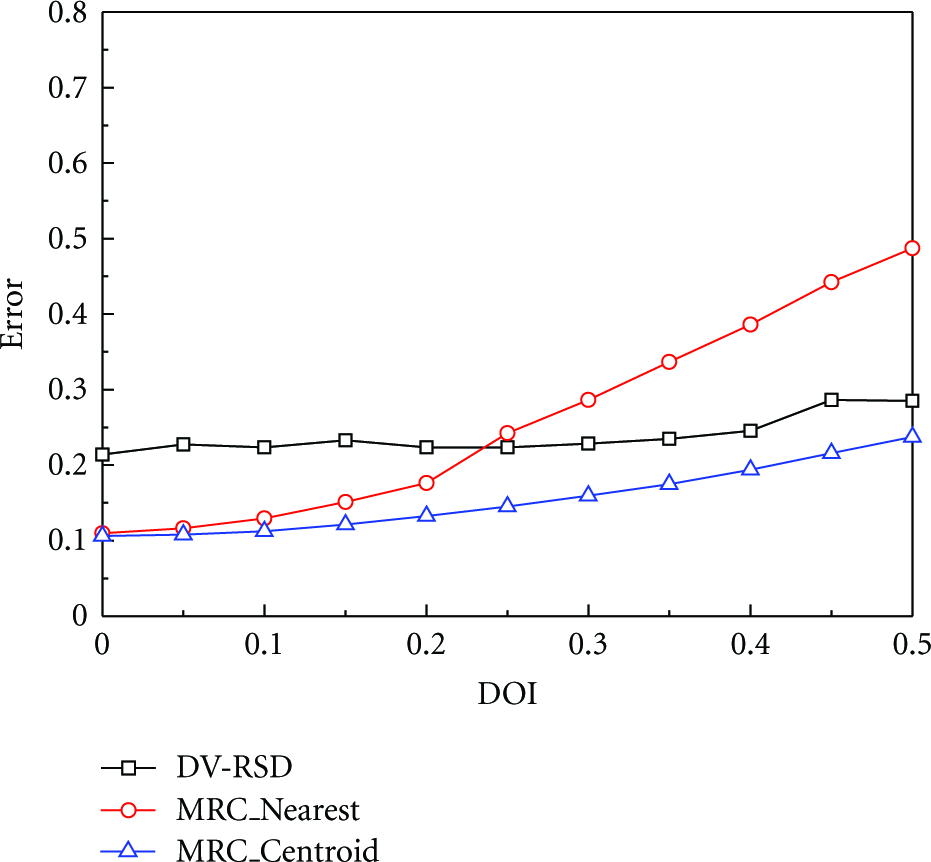
Compared with RSS-assisted localization with noise.

5. Physical Evaluation

In this section, we give the physical evaluation of our localization algorithms in the outdoor environment. 50 MicaZ sensor nodes were randomly deployed $250 \times 250$ feet square area in the school playground. Each unknown node, including mobile beacon carried by the testers, was left 10 inches above the ground with antennas pointing to the sky. The radio sending power was 0 dBm at channel 26 ( $F_{c} = 2480$ MHz) to avoid possible WiFi interference from the surroundings [2]. When the unknown node received a packet from the mobile beacon, it logged the sensed signal strength and the position of mobile beacon into its flash memory.

First, we measure the maximum distance (in feet) of 1-hop between unknown nodes in this special practical environment. The result of this measurement shows that 1-hop radio range varies from about 94 feet to 103 feet among different unknown node pairs along diverse directions. As shown in Section 3.2, the minimum distance between the transmitted beacon points is equal to 1-hop radio range. To this end, the distance between any two adjacent beacon positions of movement is 100 feet in this scenario, and DOI mentioned in Section 4.4 is less than 0.1.

Figure 16 shows the comparison of accuracy for MRC under simulation and physical environments. In general, in MRC within all different environments, error decreases as the time increases. The results of MRC ( $DOI = 0$ ) and MRC ( $DOI = 0.1$ ) are obtained in the simulation environment, and MRC (physical) is obtained in the outdoor environment. All these curvature of the curves are very similar to each other. The results remaining unchanged denote the end of localization. When the accuracy of all experiments keeps stable, results have no significant differences between simulation and physical environment; that is, MRC localization algorithm performs well in the actual environment.

Figure 16

Compared with simulation and physical experiments.

6. Conclusion

We propose a distributed MRC localization approach with a specific trajectory in static WSNs. To ensure that MRC performs as true to reality as possible, we propose two improved approaches based on MRC to consider irregular radio scenario in the noisy environment. Evaluation shows that MRC_Centroid is more robust than MRC_Nearest. Comparing the performance with three typical range-free localization methods, our lightweight MRC algorithm with limited computation and storage overhead is more suitable for very low-computing power sensor nodes that can efficiently outperform better with only basic arithmetic operations in the ideal or irregular radio model. As future work, more practical factors will be considered, and different practical factors may affect efficiency, accuracy, and flexibility of our localization approaches.

Footnotes

Acknowledgments

This work is supported by the Key Science and Technology Innovation Team Constructive Projects of Zhejiang province, China under Grant no. 2009R50009 and also supported by the National Basic Research Program of China (973 Program) under Grant no. 2006CB303000.

References

Yick

Mukherjee

Ghosal

Wireless sensor network survey

Computer Networks 2008 52 12 2292 2330

2-s2.0-46449122114

10.1016/j.comnet.2008.04.002

Zhong

Achieving range-free localization beyond connectivity

Proceedings of the 7th ACM Conference on Embedded Networked Sensor Systems, (SenSys '09)

November 2009

Berkeley, Calif, USA

281 294

2-s2.0-74549122106

10.1145/1644038.1644066

Zhongwen

Ying

Feng

Xiaohui

Yuan

Yunhao

Perpendicular intersection: locating wireless sensors with mobile beacon

Proceedings of the Real-Time Systems Symposium, (RTSS '08)

December 2008

Barcelona, Spain

93 102

2-s2.0-67249139792

10.1109/RTSS.2008.16

Hofmann-Wellenhof

Lichtenegger,

Collins

Global Positioning System: Theory and Practice 1997 4th

New York, NY, USA

Springer

Lanzisera

Lin

D. T.

Pister

K. S. J.

RF time of flight ranging for wireless sensor network localization

Proceedings of the 4th Workshop on Intelligent Solutions in Embedded Systems, (WISES '06)

June 2006

Vienna, Austria

165 176

2-s2.0-36148962051

10.1109/WISES.2006.234736

Priyantha

N. B.

Chakraborty

Balakrishnan

Cricket location-support system

Proceedings of the 6th Annual International Conference on Mobile Computing and Networking (MOBICOM '00)

August 2000

Boston, Mass, USA

32 43

2-s2.0-0034539094

Savvides

Han

C. C.

Strivastava

M. B.

Dynamic fine-grained localization in ad-hoc networks of sensors

Proceedings of the 7th Annual International Conference on Mobile Computing and Networking

July 2001

Rome, Italy

166 179

2-s2.0-0034775930

Cheng

Thaeler

Xue

Chen

TPS: a time-based positioning scheme for outdoor wireless sensor networks

Proceedings of the 23rd Annual Joint Conference of the IEEE Computer and Communications Societies

2004

Hong Kong

2685 2696

Niculescu

Nath

Ad hoc positioning system (APS) using AOA

Proceedings of the 22nd Annual Joint Conference of the IEEE Computer and Communications

2003

San Francisco, Calif, USA

1734 1743

10.

Chang

Tian

Lai

Chu

Huang

Spinning beacons for precise indoor localization

Proceedings of the 6th ACM Conference on Embedded Network Sensor Systems

2008

Raleigh, NC, USA

127 140

11.

Bahl

Padmanabhan

V. N.

RADAR: an in-building RF-based user location and tracking system

Proceedings of the 14th Annual Joint Conference of the IEEE Computer and Communications Societie

2000

Tel Aviv, Israel

775 784

12.

Costa

J. A.

Patwari

Hero

A. O.

Distributed weighted-multidimensional scaling for node localization in sensor networks

ACM Transactions on Sensor Networks 2006 2 1 39 64

2-s2.0-33745240949

10.1145/1138127.1138129

13.

Varshavsky

de Lara

Hightower

LaMarca

Otsason

GSM indoor localization

Pervasive and Mobile Computing 2007 3 6 698 720

2-s2.0-35648972001

10.1016/j.pmcj.2007.07.004

14.

Yedavalli

Krishnamachari

Sequence-based localization in wireless sensor networks

IEEE Transactions on Mobile Computing 2008 7 1 81 94

2-s2.0-36549073131

10.1109/TMC.2008.4387797

15.

Zhang

Shan

Ranking-Based statistical localization for wireless sensor networks

Proceedings of the IEEE Wireless Communications and Networking Conference, (WCNC '08)

April 2008

Las Vegas, Nev, USA

2561 2566

2-s2.0-51649118387

16.

Bulusu

Heidemann

Estrin

GPS-less low-cost outdoor localization for very small devices

IEEE Personal Communications 2000 7 5 28 34

2-s2.0-0034291601

10.1109/98.878533

17.

Huang

Blum

B. M.

Stankovic

J. A.

Abdelzaher

Range-free localization schemes for large scale sensor networks

Proceedings of the 9th Annual International Conference on Mobile Computing and Networking, (MobiCom '03)

September 2003

San Diego, Calif, USA

81 95

2-s2.0-1542329081

18.

Niculescu

Nath

DV based positioning in Ad Hoc networks

Telecommunication Systems 2003 22 1-4 267 280

2-s2.0-0038703640

10.1023/A:1023403323460

19.

Shang

Ruml

Improved MDS-based localization

Proceedings of the 23rd Annual Joint Conference of the IEEE Computer and Communications Societies

2004

Hong Kong

2640 2651

20.

Shi

A SDP approach for range-free localization in wireless sensor networks

Proceedings of the IEEE International Conference on Communications, (ICC '08)

May 2008

Beijing, China

4214 4218

2-s2.0-51249113171

10.1109/ICC.2008.791

21.

Römer

The Lighthouse Location System for Smart Dust

Proceedings of the 1st International Conference on Mobile systems, Applications and Services

2003

San Francisco, Calif, USA

15 30

22.

Stoleru

Stankovic

J. A.

Luebke

A High-accuracy, low-cost localization system for wireless sensor networks

Proceedings of the 3rd International Conference on Embedded Networked Sensor Systems

2005

San Diego, Calif, USA

13 26

23.

Xiao

Chen

Zhou

A walking beacon-assisted localization in wieless sensor networks

Proceedings of the IEEE International Conference on Communications

2007

Glasgow, Scotland

3070 3075

10.1109/ICC.2007.510

24.

Teng

Zheng

Dong

An efficient and self-adapting localization in static wireless sensor networks

2009 9

Sensors

8 6150 6170

10.3390/s90806150

25.

Huang

Záruba

G. V.

Static path planning for mobile beacons to localize sensor networks

Proceedings of the 5th Annual IEEE International Conference on Pervasive Computing and Communications Workshops, (PerCom '07)

March 2007

New York, NY, USA

323 328

2-s2.0-34547660363

10.1109/PERCOMW.2007.109

26.

Rudafshani

Datta

Localization in wireless sensor networks

Proceedings of the 6th International Symposium on Information Processing in Sensor Networks (IPSN '07)

April 2007

Cambridge, Mass, USA

51 60

2-s2.0-35348855583

10.1145/1236360.1236368

27.

Arulampalam

M. S.

Maskell

Gordon

Clapp

A tutorial on particle filters for online nonlinear/non-Gaussian Bayesian tracking

IEEE Transactions on Signal Processing 2002 50 2 174 188

2-s2.0-0036475447

10.1109/78.978374

28.

Evans

Localization for mobile sensor networks

Proceedings of the 10th Annual International Conference on Mobile Computing and Networking (MobiCom '04)

October 2004

New York, NY, USA

45 57

2-s2.0-11244273945

29.

Sichitiu

M. L.

Ramadurai

Localization of wireless sensor networks with a mobile beacon

Proceedings of the IEEE International Conference on Mobile Ad-Hoc and Sensor Systems

October 2004

Philadelphia, Pa, USA

174 183

2-s2.0-20344396105

30.

Priyantha

N. B.

Balakrishnan

Demaine

E. D.

Teller

Mobile-assisted localization in wireless sensor networks

Proceedings of The 24th Annual Joint Conference of the IEEE Computer and Communications Societies

2005

Miami, Fla, USA

172 183

31.

Kim

Lee

MBAL: a mobile beacon-assisted localization scheme for wireless sensor networks

Proceedings of the 16th International Conference on Computer Communications and Networks 2007, (ICCCN '07)

August 2007

Honolulu, Hawaii, USA

57 62

2-s2.0-40949083866

10.1109/ICCCN.2007.4317797

32.

Stoleru

Stankovic

J. A.

Walking GPS: a practical solution for localization in manually deployed wireless sensor networks

Proceedings of the 29th Annual IEEE International Conference on Local Computer Networks, (LCN '04)

November 2004

Tampa, Fla, USA

480 489

2-s2.0-20544473016

10.1109/LCN.2004.136

33.

Grant

Boyd

CVX: matlab software for disciplined convex programming

http://cvxr.com/cvx/

A Mobile-Beacon-Assisted Sensor Network Localization Based on RSS and Connectivity Observations

Abstract

1. Introduction

(i) Improved Connectivity Restriction

(ii) Further Neighborhood Sensing Restriction

(iii) Lightweight Computation and Storage

2. Related Works

3. Design

3.1. MRC Localization Scheme

3.2. Trajectory of Mobile Beacon

3.3. Regular Radio Model

(1) Beacon Acquisition

(2) Region Determination

Case 1 (3-connectivity).

Case 2 (4-connectivity).

Case 3 (7-connectivity).

(3) Location Calculation

Case 1 (3-connectivity).

Case 2 (4-connectivity).

3.4. Irregular Radio Model

Case 1 (less than or equal to 2-connectivity).

Case 2 (3-connectivity).

Case 3 (4-connectivity).

Case 4 (greater than or equal to 5-connecitvity).

4. Simulation Evaluation

4.1. Assumption

4.2. Compared with Classic Range-Free Localization Approaches

4.2.1. Localization Error When Varying Unknown Node Density

Random Deployment of Beacons

Regular Deployment of Beacons

4.2.2. Localization Error When Varying DOI

Random Deployment of Beacons

Regular Deployment of Beacons

4.3. Compared with Connectivity-Based Mobile-Beacon-Assisted Range-Free Localization Approaches

4.3.1. Localization Error As the Time Increased without Noise

4.3.2. Localization Error When Varying DOI

4.4. Compared with RSS-Assisted Range-Free Localization Approaches

4.4.1. Localization Error As Beacons Increased without Noise

4.4.2. Localization Error When Varying Unknown Node Density

4.4.3. Localization Error When Varying DOI

5. Physical Evaluation

6. Conclusion

Footnotes

Acknowledgments

References