Sage Journals: Discover world-class research

Abstract

An ANN model is proposed to predict the impurity concentration in solid diffusion process when the diffusion coefficient is not known using back-propagation learning technique based on insufficient data for analytical solution. The proposed model was very competitive against the analytical method as the results showed high-performance results with minimal amount of error comparing to the analytical method. Moreover, the proposed ANN model can be used where the analytical methods cannot as in some situations wherethe diffusion coefficient is not available

1. Introduction

The random jump of atoms of solute species with respect to the atoms of the host crystal is the core concept of diffusion. This kind of mass transfer of atoms takes place in gaseous, liquid, and solid states [1, 2]. The movement of point defects within the solid is the mechanism by which atoms move within the solid structure of the material. In general, there are two acting techniques of diffusion in solids. The first type is the interstitial diffusion method which requires the jump of the impurity from one place to another. The second type of atoms diffusion tacks place in the substitution solid solution and requires vacancy on the lattice site adjacent to it. Such movement of atoms demands a driving force to occur [2, 3]. At the same time, the diffusion rate will be stimulated at higher temperature and depends on the packing factor of the host's structure as well. Therefore, it is being more rapid for less densely packed structure. Despite that diffusion process is considered as a natural phenomenon, it finds its way through many engineering applications [4]. Spot welding uses the diffusion phenomenon to joint or bond metals together. Steel carburization manufacturing adopts the diffusion process to produce a wear resistance surface. Microelectronics industries are using the diffusion process by doping impurities into Si wafers intentionally. Turbine blades coating and sintering of powder metal are other examples of the controlled diffusion environments and applications.

In general, there are four types of diffusion. The first type is self-diffusion which represents the movement of atoms within a pure material on the absence of a concentration gradient. The second type is the tracer diffusion which is similar to self-diffusion except that some of the atoms of the host element or ion are radioactive isotopes. It should be noted that there is no direct method for measuring the self-diffusion or tracer diffusion coefficient [3, 4]. The third type of diffusion is intrinsic diffusion which refers to the mobility of a species in a binary solid. It considers that each species possesses an intrinsic diffusion coefficient. The fourth type is the mutual or chemical diffusion which occurs in presence of concentration gradient driving force and results in net transport of mass. The diffusion coefficients of the third and the fourth types are related by Darken equation, and both obey Fick's law of diffusion [1, 3, 4].

2. Analytical Analysis of Solid Diffusion

The driving forces of the atomic migrations are concentration, temperature, or electrical field gradients. Fick's first law describes the net diffusion flux down the concentration gradient as a relationship between the concentration gradient driving force, the jump distance, and the jump frequency. The relationship between these variables is presented by the following equation [1, 2, 4]:

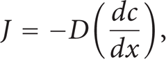
\begin{matrix} J = - D (\frac{d c}{d x}), \end{matrix}

(1)

where J: the net diffusion flux of atoms in a specific x direction at constant temperature, dc / dx: the concentration gradient, and D: the diffusion coefficient.

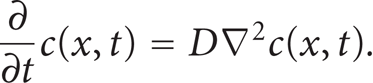
When the concentration of the diffused specie varies with time at any location within the host crystal, the mathematical model of the diffusion process can be modeled by Fick's Second law

\begin{matrix} \frac{\partial}{\partial t} c (x, t) = D \nabla^{2} c (x, t) . \end{matrix}

(2)

The stochastic nature of the diffusion process can be presented as a probability density function to find the particle with a certain velocity at any time and any position. Einstein model of diffusion connects the macroscopic property of the diffusion coefficient with the microscopic properties of the jump frequency and the jump distance [2, 4]. In one dimension, the frequency with which an impurity atom jumps from an equilibrium site to a particular adjacent equilibrium site is formulated as follows:

D = λ^{2} w

(3)

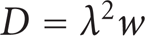
where w: the jump frequency, λ : the jump distance.

When applying the previous equation on three dimensions, it yields [2, 4]

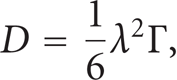
\begin{matrix} D = \frac{1}{6} λ^{2} Γ, \end{matrix}

(4)

where Γ: total jump frequency.

Boltzmann's factor is (e^-ε/kT), which expresses the probability of a state of energy, ε, relative to the probability of a state of zero energy. This factor shows up in situations where the temperature, T, is given. It is proportional to the probability that the system is in a state with energy, ε. From statistical point of view, the Boltzmann factor represents the fraction of the vibrations of the impurity atom that succeed in overcome the energy barrier [2, 4]. The jump frequency can be formulated as

\begin{matrix} w = v e^{- ε / k T}, \end{matrix}

(5)

where ε: the energy barrier of the system, v: the vibration frequency of the impurity atom in its equilibrium site, and k: Boltzmann's constant.

The vibration frequency, v, can be calculated by expanding thepotential energy curve,U(x), at the equilibrium site which yield to a simple harmonic motion with an oscillationfrequency

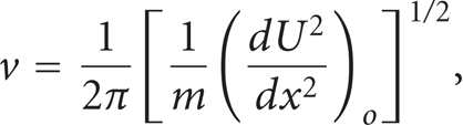
\begin{matrix} v = \frac{1}{2 π} {[\frac{1}{m} {(\frac{d U^{2}}{d x^{2}})}_{o}]}^{1 / 2}, \end{matrix}

(6)

where m: the mass of the impurity atom.

A reasonably accurate estimate of ν can be obtained by approximating the potential energy function as a sinusoid of amplitude ε and wave length λ,

\begin{matrix} v = \frac{1}{\sqrt{2}} {(\frac{ε}{m λ^{2}})}^{1 / 2} . \end{matrix}

(7)

If cubic lattices have been considered, the jump distance is a fraction of the lattice constant such that

\begin{matrix} λ = f a_{o} \end{matrix}

(8)

where f: afraction of the lattice constant, a_o: the lattice constant.

The total jump frequency is a multiple β of the one-way jump frequency, Γ = βw. Based on the above equations, the diffusion coefficient can be formulated as:

\begin{matrix} D = \frac{f β}{6 \sqrt{2}} a_{o} \sqrt{\frac{ε}{m}} e^{- ε / k T} . \end{matrix}

(9)

The diffusion coefficient D contains the temperature at which the atoms attempt to jump from plane to another as well as the interplanar distance is a function of the crystal structure [5, 6]. Considering the link between the Boltzmann constant and the universal gas constant,

\begin{matrix} R = N k, \end{matrix}

(10)

where N: Avogadro constant, R: universal gas constant.

The diffusion coefficient can be formulated as Arrhenius form regardless of the atomic mechanism which is responsible of the atom's mobility [4, 7]. The Arrhenius form of diffusion coefficient is presented by

\begin{matrix} D = D_{o} e^{(- Q / R T)}, \end{matrix}

(11)

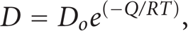
where D_o: exponential constant, Q: the activationenergy, R: universal gas constant, and T: the absolute temperature.

Based on (2), the concentration at location, x, and at the given time, t, can be obtained by

\begin{matrix} (\frac{C (x, t) - C_{o}}{C_{s} - C_{o}}) = 1 - \erf (\frac{x}{2 \sqrt{D t}}), \end{matrix}

(12)

where C_s:the concentration of the surface, C_o:the initial bulk concentration, t: the time, x: the location at a particular instant, andD: diffusion coefficient.

And the error function is defined as shown in Figure 1.

Figure 1:

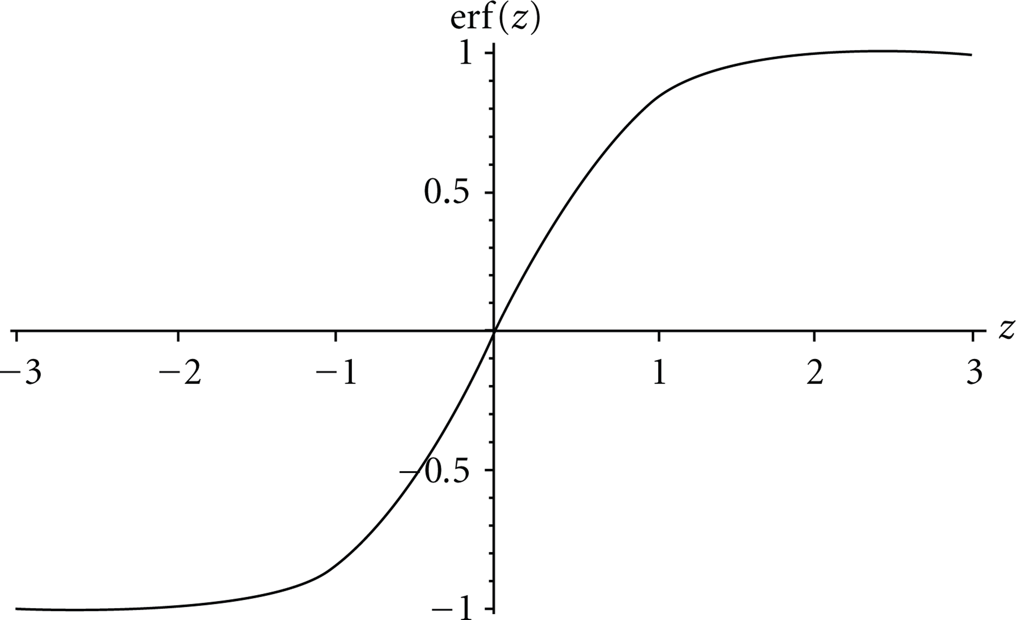
The error function used in the concentration model.

3. Research Significance

As mentioned earlier, the analytical approach to determine the concentration at any given location and time requires prior knowledge about the diffusion coefficient which varies with temperature and the microstructure of the host material. On the other hand, the diffusion processes which are not amenable to any closed-form analytical solution are difficult to analyze.

Not many literatures have been devoted to estimate the impurity concentration in solid diffusion using ANN. Moreover, none of them included most of the factors involved in the diffusion in their estimation process. Therefore, the aim of this research is to develop a useful and practical ANN model that utilizes most of the factors involved in the diffusion process to predict the concentration of impurities in solid diffusion [8–10].

The intended network should possess the capability to predict the concentration of the impurity species at any poison and time through training in premeasured quantities. This training will rely on the past experience solo. The network will model the diffusion process based on simulated or laboratory measured values. Accordingly, the relationship between the diffusion's input parameters and the output will be established. The prior knowledge of the diffusion coefficient will be redundant or unnecessary factor to predict the concentration of impurity according to the input parameters. The input vector of the intelligent network should represent the effective variables of the diffusion process.

4. Simulating Diffusion Process Based onIntelligent Networks

Artificial neural network (ANN) is a powerful data modeling tool especially when the model has three or more variables [11, 12]. It has the ability to learn both linear and nonlinear relationships between many variables directly from a set of tests, examples, and field information. It allows a reasonable application of the model to unlearned data. Artificial neural network has been used to estimate many material properties, and it has a wide range of applications in the mechanical engineering field [13–16]. The heart of the ANN is the learning algorithm that tunes its weights. One of the most widely used learningalgorithms is the back-propagation learning technique that was proposed by Paul Werbos in 1974. The back-propagation algorithm trains the ANN model how to conduct certain tasks. It uses the error between what is desired and what is actual (generated by the ANN) to adjust the weights for the model.

Assume that there are P input vectors, Z, then let C _p be the actual concentrationof the impurity for any given input vector Z _P . For any training pair {Z _p , C _p }, the back-propagation algorithms will be applied to tune the weights of the model as follows: by introducing Z _p to the input nodes, The corresponding output, O _p , will be computed by the output nodes. The difference between the desired, C _p , and the neurons response, O _p , will set the base for learning process. Accordingly, the weight of the hidden and output layers will be updated.

The architecture shown in Figure 2 represents the proposed ANN model for predicting impurity concentration based on error back-propagation network. For a certain plat, the input vector, Z is consisting of the following measured parameters:

\begin{matrix} Z = {(T, C_{s}, C_{o}, t, x)}^{t}, \end{matrix}

(13)

where T:the absolute temperature, C_s:the concentration of the surface, C_o:the initial bulk concentration, t: the time, and x:the location at a particular instant.

Figure 2:

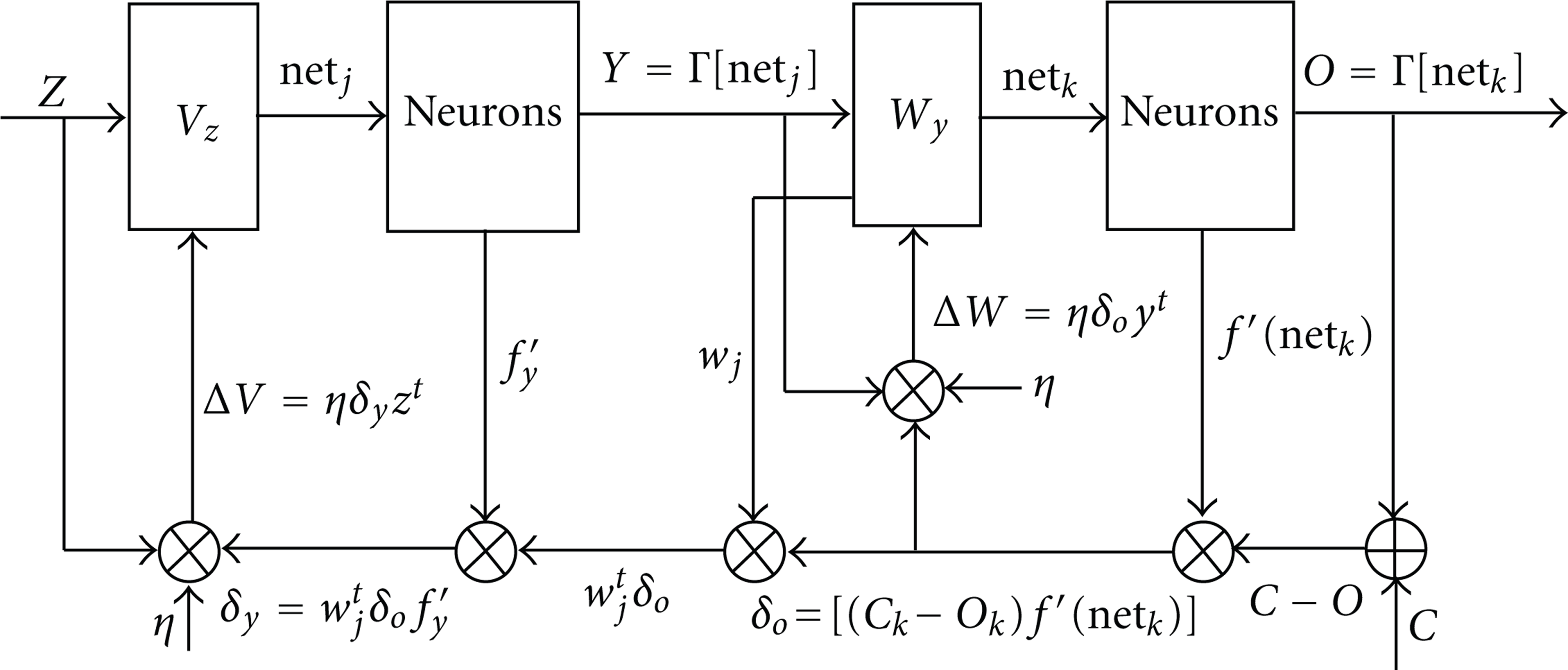
ANN model for predicting carbon concentration using error back-propagation training algorithm.

5. Network Implementation

The proposed algorithm was applied to measure the carbon concentration beneath the surface of iron bars to produce a wear resistance surface. The data, which consists of three different groups, was generated analytically utilizing a MATLAB code using the temperature, the initial concentration of the carbon in the iron bars, the surface concentration in CO/CO₂ gas environments, the depth beneath the surface, and the timeas the input parameters for calculating the carbon concentrations [17, 18]. The first group was used for training purposes as shown in Table 1. The second group, which is presented in Table 2, was used for testing the training processes. The third group, which is presented in Table 3, was used for validating the network solution by comparing the predicted carbon concentrations at the output node with those that were generated analytically by the MATLAB code.

Table 1:

Training points.

T	C _s	C _o	x	t	C(x, t)	Trained output

1000	0.003	0.001	1.00E-05	10	0.001021104	0.000893197
1000	0.003	0.001	3.00E-05	500	0.00155591	0.001447321
1000	0.003	0.001	5.00E-05	10	0.001	0.000936371
1000	0.003	0.001	5.00E-05	1000	0.001402079	0.001494953
1000	0.005	0.002	1.00E-05	500	0.00415286	0.004010624
1000	0.005	0.002	3.00E-05	1000	0.003328963	0.003552278
1000	0.005	0.002	5.00E-05	500	0.002211722	0.002333728
1000	0.007	0.004	1.00E-05	10	0.004031656	0.004148417
1000	0.007	0.004	3.00E-05	500	0.004833865	0.004923466
1000	0.007	0.004	5.00E-05	10	0.004	0.003829192
1000	0.007	0.004	5.00E-05	1000	0.004603118	0.004723393
1400	0.003	0.001	1.00E-05	500	0.002949705	0.002784246
1400	0.003	0.001	3.00E-05	10	0.002007378	0.002131236
1400	0.003	0.001	5.00E-05	500	0.002749523	0.002622404
1400	0.005	0.002	1.00E-05	10	0.004470842	0.004559702
1400	0.005	0.002	1.00E-05	1000	0.00494665	0.004858178
1400	0.005	0.002	3.00E-05	500	0.004773974	0.004621858
1400	0.005	0.002	5.00E-05	1000	0.00473378	0.004571284
1400	0.007	0.004	1.00E-05	500	0.006924558	0.006868145
1400	0.007	0.004	3.00E-05	10	0.005511066	0.005547994
1400	0.007	0.004	3.00E-05	1000	0.006840056	0.006827482
1700	0.003	0.001	1.00E-05	10	0.002878894	0.00277619
1700	0.003	0.001	1.00E-05	1000	0.002987878	0.003022788
1700	0.003	0.001	3.00E-05	500	0.002948579	0.003019181
1700	0.003	0.001	5.00E-05	1000	0.002939403	0.002719695
1700	0.005	0.002	1.00E-05	500	0.004974285	0.005028109
1700	0.005	0.002	3.00E-05	1000	0.004945455	0.004875396
1700	0.005	0.002	5.00E-05	500	0.004871486	0.004843299
1700	0.007	0.004	1.00E-05	10	0.006818341	0.006641503
1700	0.007	0.004	5.00E-05	10	0.006112227	0.006322457
1700	0.007	0.004	5.00E-05	1000	0.006909105	0.007031836

Where T is the absolute temperature, C_s is the concentration of the surface, C_o is the initial bulk concentration, x is the location at a particular instant in (m), and t is time in (s).

Table 2:

Test points.

T	C _s	C _o	x	t	C(x, t)	Trained output

1000	0.003	0.001	1.00E-05	500	0.00243524	0.002193021
1000	0.003	0.001	3.00E-05	1000	0.001885976	0.002613637
1000	0.005	0.002	1.00E-05	10	0.002031656	0.002259055
1000	0.005	0.002	3.00E-05	500	0.002833865	0.002709872
1000	0.005	0.002	5.00E-05	1000	0.002603118	0.002873281
1000	0.007	0.004	3.00E-05	10	0.004	0.003901116
1400	0.003	0.001	1.00E-05	1000	0.002964433	0.003116136
1400	0.003	0.001	5.00E-05	10	0.001530134	0.001642907
1400	0.005	0.002	1.00E-05	500	0.004924558	0.005083696
1400	0.005	0.002	3.00E-05	1000	0.004840056	0.004683202
1400	0.007	0.004	1.00E-05	10	0.006470842	0.005960425
1400	0.007	0.004	5.00E-05	1000	0.00673378	0.006558448
1700	0.003	0.001	3.00E-05	10	0.002639456	0.002546578
1700	0.003	0.001	5.00E-05	500	0.002914324	0.002809105
1700	0.005	0.002	1.00E-05	1000	0.004981817	0.004810107
1700	0.005	0.002	5.00E-05	10	0.004112227	0.004009713
1700	0.007	0.004	1.00E-05	500	0.006974285	0.007228117
1700	0.007	0.004	3.00E-05	1000	0.006945455	0.007315776

Where T is the absolute temperature, C_s is the concentration of the surface, C_o is the initial bulk concentration, x is the location at a particular instant in (m), and t is time in (s).

Table 3:

Validation points.

T	C _s	C _o	x	t	C(x, t)	Trained output

1400	0.005	0.002	3.00E-05	10	0.003511066	0.003852316
1400	0.005	0.002	5.00E-05	500	0.004624284	0.004009074
1400	0.007	0.004	1.00E-05	1000	0.00694665	0.006678362
1400	0.007	0.004	5.00E-05	10	0.004795201	0.004521251
1700	0.003	0.001	1.00E-05	500	0.002982857	0.002687671
1700	0.003	0.001	3.00E-05	1000	0.002963636	0.002894205
1700	0.005	0.002	1.00E-05	10	0.004818341	0.004794532
1700	0.005	0.002	3.00E-05	500	0.004922868	0.004668448
1700	0.005	0.002	5.00E-05	1000	0.004909105	0.004769539
1700	0.007	0.004	3.00E-05	10	0.006459184	0.006638639
1700	0.007	0.004	5.00E-05	500	0.006871486	0.007191807

Where T is the absolute temperature, C_s is the concentration of the surface, C_o is the initial bulk concentration, x is the location at a particular instant in (m), and t is time in (s).

6. Results

By feeding the input parameters to the input nodes of the ANN model, the learning process starts based on the available data. As Figure 3 shows, the error dropped to 2.4×10^{− 5} after 24 epochs. The figure shows a perfect agreement between the training, the test, and the validation sets.

Figure 3:

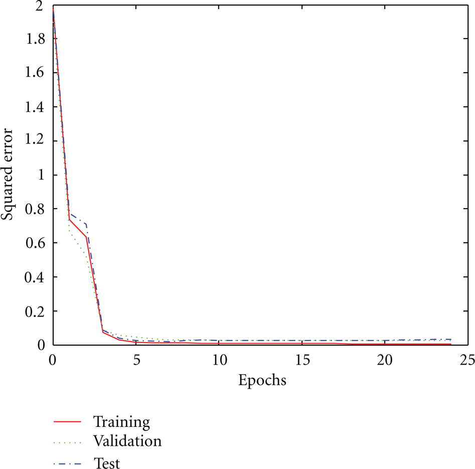
Training epoch verses error.

Figure 4 compares between the values of the concentrations generated analytically and between concentrations found by the proposed model. The correlation coefficient between the analytically generated and the ANN model predicted concentration values is 0.992. This suggests a very strong positive relationship between them which indicates that the ANN model is applied to predict the concentrations precisely. The best line that fits the predicted and the analytically generated concentrations was found to be

A = 0.993 T + 2.42 \times 10^{- 5} .

(14)

Figure 4:

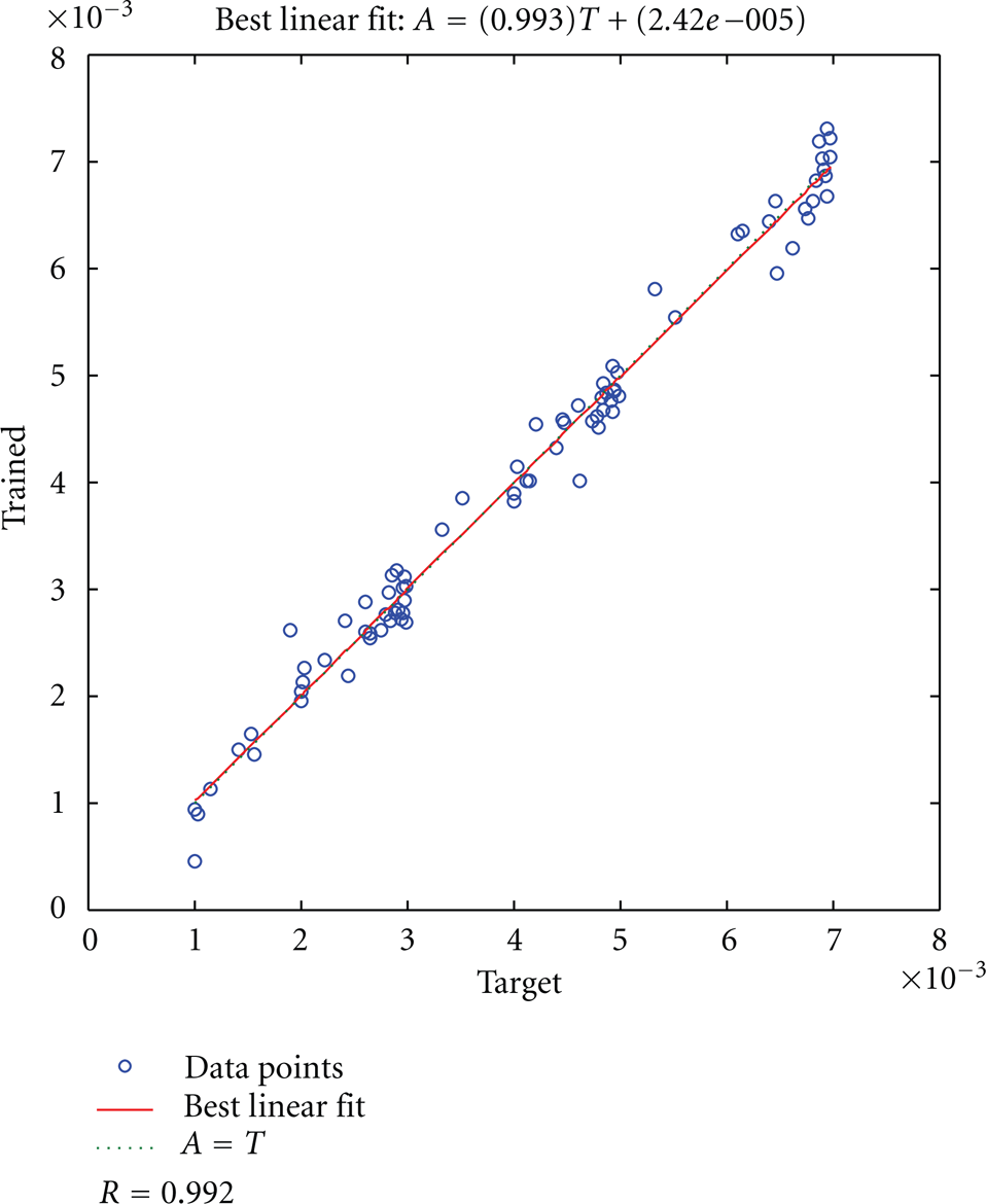
The target versus trained.

7. Advantages and Limitations

It is well known that the analytical model for diffusion requires knowledge of the structure of the host material. The activation energy for diffusion is a function of many components; therefore, it is very difficult to estimate. To calculate the exponential constant, the information of the lattice parameters, the atomic vibration frequency, and the physical property of the host as well as the impurity material need to be available, while the ANN model relays on the experimentally measured data and does not need such information. The relationship between the input and the output variables in the ANN model is established through training iterations based on the available information. The drawback of ANN model is that it needs significant amount of premeasured data to minimize the error of the predicted concentration level of the impurity.

8. Conclusion

The proposed ANN model for calculating the concentrations of impurities approaches the problem from a practical point of view as it depends on premeasured data of certain measured parameters to predict the concentration of the impurity species at different location and time with respect to diffusion process initial parameters without the need for the prior knowledge of the diffusion coefficient, which is hard to know in some cases. This renders this way of estimating the impurity concentrations more flexibile over the analytical approach. The proposed model for predicting impurity concentrations was very competitive against the analytical method as the results showed high-performance results with minimal amount of error comparing to the analytical method. Moreover, the proposed ANN model can be used where the analytical methods cannot, as in some situations where the diffusion coefficient is not available.

References

Shewmon

, Diffusion in Solids, The Minerals, Metals & Materials Society, 2nd edition, 1989.

Crank

, The Mathematics of Diffusion, Clarendon Press, Oxford, UK, 2nd edition, 1975.

Philibert

, Atom Movements: Diffusion and Mass Transport in Solids, De Physique, Les Ulis, France, 1991.

Glicksmann

M. E.

, Diffusion in Solids: Field Theory, Solid State Principles and Applications, Wiley, New York, NY, USA, 2000.

Raspo

Nicolas

Neau

, and Meradji

, “Diffusion coefficients of solids in supercritical carbon dioxide: modelling of near critical behaviour,” Fluid Phase Equilibria, vol. 263, no. 2, pp. 214–222, 2008.

Leblond

J. B.

, “Mathematical results for a model of diffusion and precipitation of chemical elements in solid matrices,” Nonlinear Analysis: Real World Applications, vol. 6, no. 2, pp. 297–322, 2005.

Dickinson

C. F.

and Heal

G. R.

, “Solid-liquid diffusion controlled rate equations,” Thermochimica Acta, vol. 340–341, pp. 89–103, 1999.

Ochoa-Martínez

C. I.

Ramaswamy

H. S.

, and Ayala-Aponte

A. A.

, “ANN-based models for moisture diffusivity coefficient and moisture loss at equilibrium in osmotic dehydration process,” Drying Technology, vol. 25, no. 5, pp. 775–783, 2007.

Taskin

Dikbas

, and Caligulu

, “Artificial neural network (ann) approach to prediction of diffusion bonding behavior (shear strength) of ni-ti alloys manufactured by powder metalurgy method,” Mathematical and Computational Applications, vol. 13, no. 3, pp. 183–191, 2008.

10.

Peng

, and Ma

, “Neural network analysis of chloride diffusion in concrete,” Journal of Materials in Civil Engineering, vol. 14, no. 4, pp. 327–333, 2002.

11.

Lippmann

R. P.

, “Introduction to computing with neural nets,” IEEE ASSP Magazine, vol. 4, no. 2, pp. 4–22, 1987.

12.

Fausett

, Fundamentals of Neural Networks: Architectures, Algorithms and Applications, Prentice Hall, Englewood Cliffs, NJ, USA, 1994.

13.

Koker

and Altinkok

, “Modelling of the prediction of tensile and density properties in particle reinforced metal matrix composites by using neural networks,” Materials and Design, vol. 27, no. 8, pp. 625–631, 2005.

14.

Taskin

and Caligulu

, “Modelling of micro-hardness values by means of artificial neural networks of Al/SiCp metal matrix composite material couples processed with diffusion method,” Mathematical and Computational Applications, vol. 11, no. 3, pp. 163–172, 2006.

15.

Perzyk

and Kochański

A. W.

, “Prediction of ductile cast iron quality by artificial neural networks,” Journal of Materials Processing Technology, vol. 109, no. 3, pp. 305–307, 2001.

16.

Rafiq

M. Y.

Bugmann

, and Easterbrook

D. J.

, “Neural network design for engineering applications,” Computers and Structures, vol. 79, no. 17, pp. 1541–1552, 2001.

17.

MATLAB–Mathworks, “MATLAB Fuzzy logic toolbox help,” 2009, http://www.mathworks.com/help/toolbox/fuzzy/index.html.

18.

Zimmermann

H. J.

, Fuzzy Set Theory and Its Applications, Kluwer Academic publisher, Boston, Mass, USA, 4th edition, 2001.

Using Artificial Neural Network for Predicting Impurity Concentration in Solid Diffusion Process under Insufficient Input Parameters

Abstract

1. Introduction

2. Analytical Analysis of Solid Diffusion

3. Research Significance

4. Simulating Diffusion Process Based onIntelligent Networks

5. Network Implementation

6. Results

7. Advantages and Limitations

8. Conclusion

References