Achieving a Realistic Notion of Time in Discrete Event Simulation

Abstract

Distributed sensor systems require clock synchronization between all sensor nodes to provide consistent view of the overall system. Owing the growing size of networks, the evaluation of the synchronization performance becomes difficult, if done by means of experiments. Simulation is another method to tackle this issue. Realistic simulation of synchronization schemes requires accurate modelling of oscillators which are the driving timers generating various events. One way to characterise oscillators is to utilize the Allan variance, which can be used to generate a phenomenological model based on power spectral density. Since discrete event simulation (DES) tools are widely used to model network protocols, models which combine accuracy and performance are needed. This paper presents a model that was optimised for use in DES. To verify that the simulation results sufficiently match measurements, an implementation in OMNeT++ was done. The results show that the behaviour of distributed sensor systems, resulting from imperfect timebases, can be accurately simulated.

1. Introduction

Common timebases in distributed sensor networks are a prerequisite for many applications in automation or instrumentation. They permit event ordering and the synchronization of actions across a network, even if these networks are not genuine real-time networks. Industrially relevant examples from the recent past are the LXI (LAN extensions for instrumentation) standard [1, 2], where IEEE 1588 [3] is used for distributed test and measurement, as well as for many industrial automation networks [4]. Sensor applications that are spatially distributed also significantly benefit from an accurate, common timebase. Examples for this are remote metering applications, data acquisition in particle accelerators, as well as structural health monitoring of bridges.

Ways to establish such a distributed timebase rely on appropriate clock synchronization strategies. Many methods have been devised and investigated in the past, such as the network time protocol (NTP) [5], the precision time protocol (IEEE 1588), or various academic approaches [6–9]. For all such synchronization approaches, evaluation of steady-state and transient performance (in terms of synchronization errors) is a central question. This is not an easy task since the processes leading to synchronization imperfections are mostly of stochastic nature and therefore difficult to describe. In some cases, analytical bounds can be found, which are however typically very coarse. Additionally, contemporary applications demand both large-scale, possibly heterogeneous networks and high accuracy. Implementations of distributed measurement and control [10] have to be evaluated (simulated) regarding their achievable performance [11] in order to show the feasibility of a networked control system as well as to optimise control algorithms. As analytical bounds may become too conservative, simulation-based behavioural investigations can come closer to the actual performance of a clock synchronization scheme.

The challenge for simulation approaches is the quality of the underlying models, and in particular the models of the oscillator as actual time reference. State-of-the-art simulators are event driven to achieve maximum performance. Compared to the time constants in a behavioural system simulation (typically in the ms range and above), an oscillator running at several 100 MHz is a continuous process which would slow down the simulation significantly if modelled in a straightforward way tick by tick. Therefore, this paper proposes a new model for oscillators combining high accuracy and efficient implementation to allow for simulation of large sensor networks with a high number of nodes.

Section 2 discusses the problem in more detail. Sections 3 and 4 are devoted to the behaviour and characterisation of oscillators and the modelling approach derived from it. Section 5 describes the actual implementation of the simulation model, and Section 6 presents an experimental verification. Finally, Section 7 draws conclusions.

2. Problem Definition

Straightforward continuous-time simulation (as done by, e.g., SPICE and its derivatives) is widely used for low-level, physical effects but has the drawback that even short simulation time spans are very compute intensive. Another technique well suited for digital systems is to assign a discrete point on a time scale to all important events and start the simulation with the occurrence of this time. This approach is usually known under the term discrete event simulators, and they are the state-of-the-art tools for network simulation (for instance ns-3 [12] or OMNeT++ [13]) or system and circuit design (like ModelSim [14]). In the case of the first two oscillators, respective clocks are modelled as a static, absolute in terms of the physical definition perfect reference to time. Thus, in order to model imperfect clocks users typically implement simple drift models where the absolute time is changed with linear models such as, for example, in the ns3::WallClockSynchronizer class of ns-3. The case is similar with ModelSim, which however provides functionality for defined delays for HDL constructs, which is applied to a, again, perfect time scale. In this case, it is also possible for the user to simulate oscillators by repetitive toggle signals. This is in standard simulations usually done using constant intervals between two transitions.

In this kind of simulation approach, systems are simulated in terms of individual events rather than a continuous time scale. These events are typically stored in a global event list, which contains the actual event and the triggering time of the event. The advantage is that this approach dynamically scales to the requirements of the simulation scenario in terms of timely resolution. For example, if one wants to simulate a distributed sensor system, which acquires data once a second, the time in between two samples does not need to be simulated in detail. However, the actual measurement and initial processing timespan could need a very fine grained simulation. Exactly this is the strength of a DES system, which tackles this by processing all events according to a virtual time scale.

The oscillator model must take into account stochastic frequency and phase variations. In addition, for DES systems, the model typically must provide the number of oscillator ticks elapsed from simulation start until any given arbitrary simulation time without actually running the simulation up to that point. Given the stochastic nature of the oscillator, this is a challenge as it has to be possible to incrementally draw samples for points which are close to each other without producing inconsistent output. It has to be noted that this modelling explicitly considers only the stochastic error, rather than parameters such as temperature dependency or errors due to vibration. The actual requirements for this simulation model therefore boil down to the following:

• (i)

the behaviour of the simulator output has to be quantised. For an oscillator model, the generated ticks have to be assigned to a discrete simulation time. This is usually no problem as it is possible to have a much finer grained simulation time scale than the actual requirements to the result. For example, the least possible difference between two events in a DES system can be picoseconds when the simulation accuracy aims at values in the nanosecond range;

(ii)

the model has to support two basic request types: it must be possible to request the number of ticks elapsed until a given simulation time and also vice versa, that is, obtain the simulation time reached by a given number of ticks;

(iii)

all data have to be consistent. Pairs of simulation time and ticks $(t,n)$ must be monotonic, that is, if $t_i>t_j\to n_i\ge n_j$ , irrespective of the order in which they are generated. Moreover, identical requests must yield identical results, that is, if $t_i=t_j\to n_i=n_j$ for a single simulation run. Therefore, requests and their answers have to be stored.

In addition, in general the always limited resources of a simulation environment have to be considered. In this sense, the most limiting factors are the available memory and the processing time. The above requirements could be easily satisfied by storing the exact time of every single oscillator tick. However, this is unfeasible due to the lack of memory. Thus, a caching strategy has to be developed where—for the sake of consistency—already calculated and scheduled events (instead of the ticks themselves) can be stored.

3. Related Work

The behaviour of an oscillator is in many ways production dependent. One key parameter is the technology. Nowadays, many types of oscillators are available, starting at low—cost AT—cut crystals used in the commonly known XOs (crystal oscillators). Here, the main influence factor on the frequency, the temperature, is neither physically stabilised nor mathematically compensated. The latter is done in the so-called microcontroller compensated oscillators (MCXOs), where the actual temperature is taken into account and the output frequency is corrected with a preconfigured temperature-frequency calibration curve. The most expensive crystal oscillators are oven controlled oscillators (OCXOs). This type of oscillators stabilises the ambient temperature of the crystal to a certain temperature. Additionally—to increase the performance—a special crystal selection process is done for the latter two types.

The actual stability of an oscillator depends on several external parameters, such as the above-mentioned temperature. Furthermore, supply voltage and mechanical effects like vibrations influence the output signal. All of these effects can be summarised in terms of their impact on the frequency stability or equivalent phase stability. The following considerations take a constant set of these parameters into account and characterise in a first step only the behaviour of an oscillator in a stable environment.

3.1. Frequency Domain Characterisation

Oscillators exhibit a variety of instabilities which are manifested in phase and frequency changes. A portion of these instabilities are well-known deterministic trends, like frequency and phase offset, drift, and periodic terms. A typical model for this is published in [15].

These instabilities cause a linear (or at most quadratic) time error term that can be easily corrected, for example, by clock synchronization with a control loop. However, for a complete model of an oscillator, it is also necessary to include the stochastic trends. According to [16], this noise can be categorised depending on the power spectral density (PSD), $S_{\phi }(f)$ , of the phase noise. The characterization with a PSD with its advantages of transformations requires a stationary noise process, which is assumed in the remainder of this paper. It is important to mention for this characterization that the underlying probability distribution is not defined by the PSD, so could white noise have a Gaussian distribution, while flicker noise may have a uniform distribution between a lower and upper limit.

(a) White Noise Family

White, bandwidth-limited noise, probably the best known noise family, is an uncorrelated, random noise process which has a constant power spectral density for all frequencies in its band. In the case of oscillators, the noise processes usually have a normal or Gaussian distribution.

In particular, two types of white noise are contributing: the commonly called white noise phase modulation (WPM, $S_{\phi }\propto 1/f^0=1$ , where f denotes the frequency) and white noise frequency modulation (WFM, $S_{\phi }(f)\propto 1/f^2$ ). The first one is frequency independent and usually denotes the phase variations which appear to be random white noise processes. Amplifiers usually contribute to this kind of noise in oscillators. Thus, by proper amplifier design, this process can be reduced. The second class of the white noise family is the white noise frequency modulation. Causes for this can be usually found in passive elements of the oscillator [17].

(b) Flicker Noise Family

This noise family is usually also referred to as pink or flicker noise, which has as its identification property a $1/f$ dependency in the PSD (power spectral density). It is characterized by equal amount of energy per octave. In oscillators, flicker noise processes can be observed in the spectrum near the resonance frequency, which results in oscillator phase noise. Similarly, like in the white family, typically two effects of flicker noise can be observed: flicker frequency modulation (FFM) and flicker phase modulation (FPM) [17].

Theories about the cause of flicker noise are relatively vague. Some sources [18] say that FPM, $1/f$ , can be related to a physical resonance mechanism in the oscillator. Usually its source is the amplification stage itself, thus it can be found even in high-quality oscillators.

The spectrum of the FFM has a power spectral density, proportional to $1/f^3$ . Its cause is again not fully investigated. Often this type is masked by WFM or FPM in lower-quality oscillators.

(c) Random Walk Noise

This noise type can be identified by its typical $1/f^4$ spectrum. It is relatively close to the carrier frequency and thus difficult to measure. However, the effect, namely the random (but directional) frequency change can be easily observed. Among the causes for this kind of noise are mechanical shock, vibration, temperature fluctuations, and similar effects [17].

More commonly the power spectral density of the frequency noise $S_y(f)$ is used (with the relation $S_y(f)=S_{\phi }(f)·f^2/v_0^2$ , where $v_0^2$ is the nominal frequency) to characterise the noise as it gives information how the average power is distributed over the frequency. Since usually the oscillator noise is modeled as a superposition of the five types of noises described above, the the PSD can be defined with the power law [19]

$S_y\left(f\right)={\displaystyle \sum }_{\alpha =-2}^2{h}_{\alpha }{f}^{\alpha },$

(1)

where $S_y(f)$ is the one-sided spectral density of the fractional frequency fluctuations (frequency noise), and $h_{\alpha }$ are constants which can be used to characterise the oscillator.

3.2. Time Domain Characterisation

In the time domain, the so-called Allan variance is used to estimate the stability of a clock. The introduction of this measure is necessary, since the classical variance diverges for a certain type, random walk noise. It is the typical effect of an oscillator's frequency to depart with variable progression and direction from the nominal frequency. As for this effect, the (temporal) mean value does not converge, also the variance does not show useful results. The Allan variance solves this issue for all noise types commonly observed in crystal oscillators. It is easy and fast to compute as well as more accurate in estimating noise processes [20–22]. The Allan variance ${\sigma }_y^2$ of the fractional relative frequency error $y(t)=1-(f(t)/f_{\text{nominal}})$ is defined by

${\sigma }_y^2\left(\tau \right)=\frac{1}{2\left(N-1\right)}{\displaystyle \sum }_{i=1}^{N-1}{\left(y_{i+1}-y_i\right)}^2.$

(2)

In this commonly used estimation, N is the number of samples. Additionally, to the division by the number of samples, the sum is divided by two so that the Allan variance is equal to the classical variance when the measured samples are uncorrelated or statistically dependent [16]. All N samples must be evenly distributed within the observation period τ. Likewise, each frequency offset can also be estimated by evaluating the time errors $x_i(t)$ . Since $y_i=(x_{i+1}-x_i)/\tau$ , the Allan variance can be also approached by evaluating

${\sigma }_y^2\left(\tau \right)=\frac{1}{2\left(M-2\right){\tau }^2}{\displaystyle \sum }_{i=1}^{M-2}{\left(x_{i+2}-2x_{i+1}+x_i\right)}^2,$

(3)

with $M=N+1$ samples of $x_i$ . Once a set of time errors has been measured over the sampling time ${\tau }_0$ , it is possible to compute the Allan variance for different sampling times $\tau =n·{\tau }_0$ . The approach is to average n adjacent values of $y_i^{{\tau }_0}$ [19],

$y_k^{\tau }=\frac{1}{n}{\displaystyle \sum }_{i=\left(k-1\right)n+1}^{k\cdot n}{y}_i^{{\tau }_0}=\frac{x_{k+n}-x_k}{\tau }.$

(4)

It is clear from the equation that the time errors for the sampling time τ are generated by skipping out $n-1$ samples. In case of a finite set of N values for $y_i^{{\tau }_0}$ , ${\sigma }_y^2(\tau )$ can be written as

${\sigma }_y^2\left(n{\tau }_0\right)=\frac{1}{2\left(M-1\right)}{\displaystyle \sum }_{k=1}^{M-1}{\left(y_{k+1}^{\tau }-y_k^{\tau }\right)}^2,$

(5)

where $M=N/n$ . This can also be done based on the time error $x_i$ when the Allan variance is defined as

${\sigma }_y^2\left(n{\tau }_0\right)=\frac{1}{2{\tau }^2\left(M-1\right)}{\displaystyle \sum }_{i=1}^{M-1}{\left(x_{\left(i+1\right)n+1}-2x_{in+1}+x_{\left(i-1\right)n+1}\right)}^2,$

(6)

for $N+1$ number of $x_i$ measurements and $M=N/n$ . $x_i$ is in this context defined as the phase offset of the oscillator to an ideal clock.

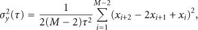
Using this algorithm, the Allan variance has become a de-facto standard to predict the quality of clocks. Nevertheless, it should be noted that for the computation of $\{x_i\}$ , a reference clock, or at least the information about its phase, is indispensable.

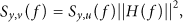
Finally, it has to be mentioned that a relationship between the time and frequency domain exists which is defined by [19]

${\tilde{\sigma }}_y^2\left(\tau \right)=2{{\displaystyle \int }}_0^{\infty }{S}_y\left(f\right)\frac{{\sin }^4\left(\pi f\tau \right)}{{\left(\pi f\tau \right)}^2}\text{d}f.$

(7)

From this representation, it is clear that one additional benefit of the Allan variance is that the type of error (modulation of the frequency) can be identified by the slope of the plot. For example, a slope of ${\tau }^{-1}$ identifies a white-phase noise (WPM) or a flicker phase (FPM). Details can be found in [20–23].

3.3. DES Clock Models

There have been attempts to bring realistic notion of time to discrete event simulation systems in literature. The main issue with DES is the one virtual time scale which is shared amongst the different components of the system, thereby making them perfectly synchronized. To make the simulation more realistic, it is necessary to introduce, as in the real world, statistically independent oscillator models every spatially distributed device. In [24], such a local clock modelling approach for DES is introduced. The clock model provides an API for other node's modules and implements several mapping utilities: (a) conversion from local time to virtual time, (b) conversion from virtual to local time, (c) conversion of local duration to virtual duration, and (d) conversion of virtual duration to local duration. With this conversions functionality, it is easy to map the nodes' notion of time to a global, absolute perfect time scale. While this solution is generic and can be easily applied in simulation, the issue of realistic clock behaviour still remains. Although the clock model exhibits most of the deterministic characteristics of real world clocks (time and frequency offset, drift, etc.), the random processes described in Section 3.1 are modelled by simple white noise which is not efficient for simulations that require high precision clock synchronization.

4. Oscillator Model Concept

Based on the considerations in the previous sections, the actual task is to model the five noise types. For this matter, the PSD of the noise can be useful, since it is deterministic and independent of time (for these certain noise types). The approach is the following.

If a random signal $u(t)$ is filtered by a linear, time-invariant filter with frequency response $H(f)$ , the power spectral density of the output signal $v(t)$ can be calculated as [25]

$S_{y,v}\left(f\right)=S_{y,u}\left(f\right){\Vert H\left(f\right)\Vert }^2,$

(8)

where $S_{y,u}(f)$ is the power spectral density of $u(t)$ , and $S_{y,v}$ refers to the power spectral density of the output signal. This fact can now be used in the following manner: in case $u(t)$ is white noise, $S_{y,u}(t)$ equals one. Therefore, the spectrum of the five types of noises can be defined which allows to define a filter cascade for white noise like in Figure 1 that has the same power spectral density as the desired oscillator noise.

Figure 1

Concept of the oscillator model. A filter, with a frequency response equal to the power spectral density of an oscillator, is used to extract similar noise behaviour from a bandwidth-limited white noise. The exact properties of the dashed box, which contains five filter elements, are developed in this section. So far, it is only important that the box as a whole forms the spectrum according to the Allan variance of the oscillator.

Therefore, the key step is to define the PSD of the noises. However, since it is easier to perform time-based measurements and, therefore, calculate the Allan variance, the relation between the Allan variance and the power spectral density has to be found.

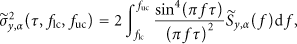
For a system with limited bandwidth, this correspondence between the Allan variance and the power spectral density is given by [16]

${\tilde{\sigma }}_y^2\left(\tau \right)=2{{\displaystyle \int }}_{f_{\text{lc}}}^{f_{\text{uc}}}{S}_y\left(f\right)\frac{{\sin }^4\left(\pi f\tau \right)}{{\left(\pi f\tau \right)}^2}\text{d}f.$

(9)

The modification concerns the always positive cutoff frequencies $f_{\text{lc}}$ and $f_{\text{uc}}$ of the measurement system. Thus, the corresponding power spectral density has to be limited to $[f_{\text{lc}},f_{\text{uc}}]$ , too. In this case of a restriction to a bandwidth-limited signal, the redefinition is simple, as only the contributing parts to $S_y(f)$ have to be cut off,

${\tilde{S}}_{y,\alpha }\left(f\right)=\{\begin{array}{cc}{h}_{\alpha }{f}^{\alpha },\hfill & \text{if}\hspace{0.17em}\hspace{0.17em}{f}_{\text{lc}}<f<f_{\text{uc}},\hfill \\ 0,\hfill & \text{otherwise}.\hfill \end{array}$

(10)

Finally, the power spectral density can be summed up to

${\tilde{S}}_y\left(f\right)={\displaystyle \sum }_{\alpha =-2}^2{\tilde{S}}_{y,\alpha }\left(f\right).$

(11)

4.1. Power Spectral Density Correspondence

Using (11), the Allan variance on a limited bandwidth, ${\tilde{\sigma }}_{y,\alpha }^2$ , is defined as

${\tilde{\sigma }}_{y,\alpha }^2\left(\tau ,f_{\text{lc}},f_{\text{uc}}\right)=2{{\displaystyle \int }}_{f_{\text{lc}}}^{f_{\text{uc}}}\frac{{\sin }^4\left(\pi f\tau \right)}{{\left(\pi f\tau \right)}^2}{\tilde{S}}_{y,\alpha }\left(f\right)\text{d}f,$

(12)

and the trivial consequence for the Allan variance is

${\tilde{\sigma }}_y^2={\displaystyle \sum }_{\alpha =-2}^2{\tilde{\sigma }}_{y,\alpha }^2\left(\tau ,f_{\text{lc}},f_{\text{uc}}\right).$

(13)

As it can be seen from inserting (10) into (12), the integral is defined only for $\alpha =-2,-\mathrm{1,0}$ . Therefore, it is mandatory to limit the upper frequency for values of $\alpha >0$ to avoid the singularity [26]. If this assumption holds, the solution of (12) for $\alpha >0$ can be given with the help of the definition of the sine integral [27]

$\mathfrak{S}\left(\zeta \right)={{\displaystyle \int }}_0^{\zeta }\frac{\sin \left(\omega \right)}{\omega }\text{d}\omega ,$

(14)

which can be approximated using a TAYLOR series around zero as

$\begin{array}{cc}\hfill \mathfrak{S}\left(\zeta \right)& =\zeta -\frac{{\zeta }^3}{3!\cdot 3}+\frac{{\zeta }^5}{5!\cdot 5}-\frac{{\zeta }^7}{7!\cdot 7}+\cdots \hfill \\ \hfill & ={\displaystyle \sum }_{k=0}^{\infty }\frac{{\left(-1\right)}^k}{\left(2k+1\right)!\cdot \left(2k+1\right)}{\zeta }^{2k+1}.\hfill \end{array}$

(15)

The second abbreviation is the cosine integral [27],

$\begin{array}{cc}\hfill \mathfrak{C}\left(\zeta \right)& =-{{\displaystyle \int }}_{\zeta }^{\infty }\frac{\cos \left(t\right)}{t}\text{d}t=\gamma +\ln \left(\zeta \right)+{{\displaystyle \int }}_0^{\zeta }\frac{\cos \left(t\right)-1}{t}\text{d}t\hfill \\ \hfill & =-{{\displaystyle \int }}_{\zeta }^0\frac{\cos \left(t\right)-1}{t}\text{d}t,\hfill \end{array}$

(16)

where $\gamma =-{\int }_0^{\infty }{e}^{-t}\ln \hspace{0.17em}(t)\text{d}t=0.577215664901532\dots$ is the Euler-Mascheroni constant [27]. Using a symbolic mathematics package and an intermediate boundary frequency $f_{\text{b}}$ which equals either $f_{\text{lc}}$ or $f_{\text{uc}}$ and introducing $u_{\text{b}}=\pi f_{\text{b}}\tau$ , the contributing parts can be written as

$\begin{array}{cc}\hfill & {\tilde{\sigma }}_{y,-2}^2\left(\tau ,0,u_{\text{b}}\right)\hfill \\ \hfill & \hspace{1em}=2{{\displaystyle \int }}_0^{u_{\text{b}}}{h}_{-2}{f}^{-2}\frac{{\sin }^4\left(\pi f\tau \right)}{{\left(\pi f\tau \right)}^2}\text{d}f\hfill \\ \hfill & \hspace{1em}=h_{-2}\pi \tau \{\phantom{\frac{{\sin }^2\left(u_{\text{b}}\right)\left[4u_{\text{b}}^2+2u_{\text{b}}\sin \left(2u_{\text{b}}\right)+\left(8u_{\text{b}}-1\right)\cos \left(2u_{\text{b}}\right)+1\right]}{3u_{\text{b}}^3}}\frac{8\mathfrak{S}\left(4u_{\text{b}}\right)-4\mathfrak{S}\left(2u_{\text{b}}\right)}{3}\hspace{0.17em}\hfill \\ \hfill & \hspace{1em}\hspace{0.5em}-\frac{{\sin }^2\left(u_{\text{b}}\right)\left[4u_{\text{b}}^2+2u_{\text{b}}\sin \left(2u_{\text{b}}\right)+\left(8u_{\text{b}}-1\right)\cos \left(2u_{\text{b}}\right)+1\right]}{3u_{\text{b}}^3}\},\hfill \end{array}$

(17)

$\begin{array}{cc}\hfill & {\tilde{\sigma }}_{y,-1}^2\left(\tau ,0,u_{\text{b}}\right)\hfill \\ \hfill & \hspace{1em}\hspace{1em}=2{{\displaystyle \int }}_0^{u_{\text{b}}}{h}_{-1}{f}^{-1}\frac{{\sin }^4\left(\pi f\tau \right)}{{\left(\pi f\tau \right)}^2}\text{d}f\hfill \\ \hfill & \hspace{1em}\hspace{1em}=h_{-1}\{\phantom{\frac{\left[4u_{\text{b}}\cos \left(u_{\text{b}}\right)+\sin \left(u_{\text{b}}\right)\right]{\sin }^3\left(u_{\text{b}}\right)}{u_{\text{b}}^2}}\ln \left(4\right)+2\mathfrak{C}\left(2u_{\text{b}}\right)-2\mathfrak{C}\left(4u_{\text{b}}\right)\hfill \\ \hfill & \hspace{1em}\hspace{1em}\hspace{1em}\hspace{1em}\hspace{1em}-\frac{\left[4u_{\text{b}}\cos \left(u_{\text{b}}\right)+\sin \left(u_{\text{b}}\right)\right]{\sin }^3\left(u_{\text{b}}\right)}{u_{\text{b}}^2}\},\hfill \end{array}$

(18)

$\begin{array}{cc}\hfill & {\tilde{\sigma }}_{y,0}^2\left(\tau ,0,u_{\text{b}}\right)\hfill \\ \hfill & \hspace{1em}=2{{\displaystyle \int }}_0^{u_{\text{b}}}{h}_0\frac{{\sin }^4\left(\pi f\tau \right)}{{\left(\pi f\tau \right)}^2}\text{d}f\hfill \\ \hfill & \hspace{1em}=h_0\frac{1}{\pi \tau }\left\{2\mathfrak{S}\left(2u_{\text{b}}\right)-\mathfrak{S}\left(4u_{\text{b}}\right)-\frac{{\sin }^4\left(u_{\text{b}}\right)}{u_{\text{b}}}\right\},\hfill \\ \hfill & {\tilde{\sigma }}_{y,1}^2\left(\tau ,0,u_{\text{b}}\right)\hfill \\ \hfill & \hspace{1em}=2{{\displaystyle \int }}_0^{u_{\text{b}}}{h}_{1}f\frac{{\sin }^4\left(\pi f\tau \right)}{{\left(\pi f\tau \right)}^2}\text{d}f\hfill \\ \hfill & \hspace{1em}=h_1\frac{1}{{\left(\pi \tau \right)}^2}\{\frac{\ln \left(4\right)+3\gamma +3\ln \left(u_{\text{b}}\right)}{4}\hfill \\ \hfill & \hspace{1em}\hspace{1em}\hspace{1em}\hspace{1em}\hspace{1em}\hspace{1em}+\frac{\mathfrak{C}\left(4u_{\text{b}}\right)-4\mathfrak{C}\left(2u_{\text{b}}\right)}{4}\phantom{\frac{\mathfrak{C}\left(4u_{\text{b}}\right)-4\mathfrak{C}\left(2u_{\text{b}}\right)}{4}}\},\hfill \\ \hfill & {\tilde{\sigma }}_{y,2}^2\left(\tau ,0,u_{\text{b}}\right)\hfill \\ \hfill & \hspace{1em}=2{{\displaystyle \int }}_0^{u_{\text{b}}}{h}_2{f}^2\frac{{\sin }^4\left(\pi f\tau \right)}{{\left(\pi f\tau \right)}^2}\text{d}f\hfill \\ \hfill & \hspace{1em}=h_2\frac{1}{{\left(\pi \tau \right)}^3}\left\{\frac{12u_{\text{b}}+\sin \left(4u_{\text{b}}\right)-8\sin \left(2u_{\text{b}}\right)}{16}\right\}.\hfill \end{array}$

(19)

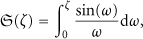
Additionally, the theorem of transposed integral limits can be used to obtain a solution for nonzero lower cutoff frequencies, that is,

${\tilde{\sigma }}_{y,\alpha }^2\left(\tau ,u_{\text{lc}},u_{\text{uc}}\right)={\tilde{\sigma }}_{y,\alpha }^2\left(\tau ,0,u_{\text{uc}}\right)-{\tilde{\sigma }}_{y,\alpha }^2\left(\tau ,0,u_{\text{lc}}\right).$

(20)

This result can be checked, by using the lemma of JORDAN to get a limit for the integralsine [27]

$\underset{\zeta \to \infty }{\lim }\mathfrak{S}\left(\zeta \right)=\frac{\pi }{2}.$

(21)

In consequence, using the fact that the second fraction ( $·/u_{\text{b}}^n$ ) of ${\tilde{\sigma }}_{y,-2}$ , ${\tilde{\sigma }}_{y,-1}$ , and ${\tilde{\sigma }}_{y,0}$ approaches zero with $u_{\text{b}}\to \infty$ , the following limits can be obtained:

$\begin{array}{c}\underset{f_{\text{b}}\to \infty }{\lim }{\tilde{\sigma }}_{y,-2}\left(\tau ,0,f_{\text{b}}\right)=h_{-2}\tau \frac{2{\pi }^2}{6},\\ \underset{f_{\text{b}}\to \infty }{\lim }{\tilde{\sigma }}_{y,-1}\left(\tau ,0,f_{\text{b}}\right)=h_{-1}\ln \left(4\right),\\ \underset{f_{\text{b}}\to \infty }{\lim }{\tilde{\sigma }}_{y,0}\left(\tau ,0,f_{\text{b}}\right)=h_0\frac{1}{2\tau },\end{array}$

(22)

which makes the result reasonable [19].

4.2. Power Spectral Density Forming

After the measurement of the Allan variance, the $h_{\alpha }$ parameters and hence the power spectral density $S_y(f)$ can be sufficiently determined. A straightforward approach would be to choose five values from the Allan variance plot and build a linear system of equations. This turns out not to be the optimal approach. Due to the imperfections of the measurement system, the calculated values of the Allan variance do not fit (18)–(20) perfectly.

A second approach is to make an approximation of the Allan variance by calculating a fitting curve using the least-square method [28]. Another way to do the approximation can be done using the infinity norm ${\parallel ·\parallel }_{\infty }$ of the error vector. The technique turns out to be the best-suited approach for the high dynamic of this double logarithmic-scaled linear problem.

The next step is to bring the PSD function of the oscillator noise into a form that the transfer function $H(s)$ can be found. By substituting $\omega =2\pi f$ , $S_y$ can be determined as

$\begin{array}{c}{S}_y\left(\omega ,{\omega }_{\text{lc}},{\omega }_{\text{uc}}\right)=\left(\frac{s_{-2}+s_{-1}\omega +s_0{\omega }^2+s_1{\omega }^3+s_2{\omega }^4}{{\omega }^2}\right)\cdot {\Pi }_{{\omega }_{\text{lc}},{\omega }_{\text{uc}}}\left(\omega \right).\end{array}$

(23)

In this equation, the boxcar function $\Pi (·)$ defines a window satisfying

${\Pi }_{{\omega }_{\text{lc}},{\omega }_{\text{uc}}}\left(\omega \right)=\{\begin{array}{cc}1,\hfill & \text{if}{\hspace{0.17em}\hspace{0.17em}\omega }_{\text{lc}}\le \omega \le {\omega }_{\text{uc}},\hfill \\ 0,\hfill & \text{otherwise.}\hfill \end{array}$

(24)

Due to the fact that the input signal of the filter is white noise, the power spectral density of the output signal is

$S_y\left(\omega ,{\omega }_{\text{lc}},{\omega }_{\text{uc}}\right)={\left|H\left(\text{j}\omega \right)\right|}^2=H\left(\text{j}\omega \right)H^{*}\left(\text{j}\omega \right),$

(25)

where $H(\text{j}\omega )$ is the transfer function of the filter. According to (24) and (26), the transfer function can now be defined as

$\begin{array}{c}\left|H\left(\text{j}\omega \right)\right|=\frac{\sqrt{s_{-2}+s_{-1}\omega +s_0{\omega }^2+s_1{\omega }^3+s_2{\omega }^4}}{\omega }\cdot {\Pi }_{{\omega }_{\text{lc}},{\omega }_{\text{uc}}}\left(\omega \right),\end{array}$

(26)

with the introduction of

$\left|P\left(\text{j}\omega \right)\right|=\frac{\sqrt{s_{-2}+s_{-1}\omega +s_0{\omega }^2+s_1{\omega }^3+s_2{\omega }^4}}{\omega }$

(27)

and factorizing the polynomial $s_{-2}+s_{-1}\omega +s_0{\omega }^2+s_1{\omega }^3+s_2{\omega }^4$ via real-valued constants ${\omega }_1\dots {\omega }_4$ such as $({\omega }_1+\omega )({\omega }_2+\omega )({\omega }_3+\omega )({\omega }_4+\omega )$ . The assumption of real coefficients is valid because the square root of the polynomial has to exist according to (27) and thus,

$\begin{array}{cc}\hfill & \left|P\left(\text{j}\omega \right)\right|\hfill \\ \hfill & \hspace{1em}\hspace{1em}=\sqrt{{\omega }_1{\omega }_2{\omega }_3{\omega }_4}\cdot \frac{\left|P_1\left(\text{j}\omega \right)\right|\left|P_2\left(\text{j}\omega \right)\right|\left|P_3\left(\text{j}\omega \right)\right|\left|P_4\left(\text{j}\omega \right)\right|}{\omega },\hfill \end{array}$

(28)

where $|P_i(\text{j}\omega )|$ is defined as

$\left|P_i\left(\text{j}\omega \right)\right|=\sqrt{\left(1+\frac{\omega }{{\omega }_i}\right)}.$

(29)

Therefore, one can consider $P(\text{j}\omega )$ as a cascade of five transfer functions: $P_1(\text{j}\omega )$ , $P_2(\text{j}\omega )$ , $P_3(\text{j}\omega )$ , $P_4(\text{j}\omega )$ , and $1/\text{j}\omega$ . The last represents an integrator with a gain $g=\sqrt{{\omega }_1{\omega }_2{\omega }_3{\omega }_4}$ : $P_{\mathrm{int}\hspace{0.17em}}=\sqrt{{\omega }_1{\omega }_2{\omega }_3{\omega }_4}/\text{j}\omega$ . The step from $|P(\text{j}\omega )|$ to $|H(\text{j}\omega )|$ is done with the assumption that the white noise input of the filter is bandwidth limited. Therefore, the limitation of the filter can be shifted to the noise source.

If one examines one of the first four parts of the cascade more closely, it is clear that it has a 10 dB/decade slope. Since it is not possible to make a filter using discrete components which has this amplitude characteristics, an approximation is needed. This can be successfully done by the lead-lag-filter [29],

$P_{\text{apr},i}\left(\text{j}\omega \right)={\displaystyle \prod }_{k=0}^{\infty }\frac{\left(1+\left(\omega /{\omega }_{\text{z},i,k}\right)\right)}{\left(1+\left(\omega /{\omega }_{\text{p},i,k}\right)\right)},$

(30)

where the zeros, ${\omega }_{\text{z},i,k}$ , and the poles, ${\omega }_{\text{p},i,k}$ , are chosen as

${\omega }_{\text{z},i,k}=2^{4k-5}\pi {\omega }_i,$

(31)

${\omega }_{\text{p},i,k}=2^{4k-3}\pi {\omega }_i,$

(32)

and $k=\mathrm{1,2},\mathrm{3,4}\dots$ are integers.

5. DES Model Implementation

Following the approach explained above, the practical implementation of the oscillator model starts with the measurement of the Allan variance and the extraction of the spectrum defining $h_{\alpha }$ parameters. An intermediate, however, necessary step in the design is to switch from the continuous time to the discrete time domain. For the sake of simplicity, this first step is done using MATLAB. This involves two tasks:

• (i)

a digital filter with the same frequency response as the analog $H(\text{j}\omega )$ has to be created. The biggest problem in this step is the wide dynamic range that the digital filter cascade has to cover. Since the dynamic frequency range of digital filters is more limited than that of analog filters, the higher frequencies are cut off to avoid stability problems;

(ii)

white noise has to be modelled. Usually white noise is modelled using random number generators providing a normal distribution.

In practice, this problem turns out to be a linear optimisation of the $h_{\alpha }$ parameters and a following construction of a proper filter. In practice, this can be also done by measuring the Allan variance and optimizing the parameters of the linear filter to match the observed PSD. This approach does not require the calculation of the $h_{\alpha }$ parameters; however, for the sake of the comparison of the parameters with the state-of-the-art s, the intermediate step is done in this paper. As mentioned already, the overall goal of the model described in this paper is to have an oscillator model available for simulation in a DES environment. However, this is not needed for the sake of itself, but the model has to be embedded into a large scope of a simulation. Owing to its high flexibility and particular suitability for network simulation, the OMNeT++ [13] simulator was chosen for a prototype implementation. It is however obvious that the model in general can be ported to other simulators as the ns-3 system or even ModelSim, as well.

5.1. OMNeT++ Model Structure

As a basis for the model, a typical clock synchronization problem is taken as test case. In this scenario, the oscillator is used as a time reference for a clock. This clock consists of the clock logic that increases the value of the clock with each tick (or couple of ticks) of the oscillator by a variable increment. By the adjustment of this increment, the clock can be steered to a desired value. This clock is then synchronized by a second, in the context of this paper ideal master clock which is per definition running perfectly aligned with the time scale of the simulation. At predefined points in time, the master clock synchronizes the slave clock. The latter then requests from the oscillator model the number of ticks elapsed since the last clock update and calculates the actual local time with the current increment. Using this and a PI-controller structure, a new increment is calculated in order to steer the slave clock according to the transmitted timestamps of the master. From an implementation viewpoint, the more complicated case is another one: for a full integration into a typical OMNeT++ simulation, it has not only to be possible to request the number of ticks at the current simulation time, but also to request the number of ticks at a given simulation time in the future (or vice versa the simulation time at a future number of ticks). This prediction is necessary, for example, to schedule clock alarms at given times when an action of the simulated system has to be performed. The latter is relatively simple in the framework because it comes down to scheduling an interrupt. However, it is not that easy for the oscillator model, since it has to be ensured that the replies to requests are consistent. This consistency is twofold: first, a repeated request has to be answered in any case with the same value, and second, it has to be ensured that the number of ticks of request 1 is always smaller or equal to the ones of request 2, given that the simulation time for the ticks in request 1 is smaller.

5.2. Power Spectral Density Shaping

As it will be shown in Section 6, the oscillator model exhibits realistic behaviour in terms of the Allan variance; however, it has to be considered whether this is sufficient for direct implementation in a DES system. One evident drawback of the model is the fact that the oscillator and, hence, local time is incremented by single, small ticks. Not only is this resource consuming in case of a network containing a large number of clocks; but also, the actual advantage of the discrete event simulation concept explained in Section 2 cannot be used properly. Therefore, following this concept, the oscillator model has to be modified in a way that it is able to simulate long periods of time efficiently and also to keep the fine granularity when needed.

Inspired by multirate filtering, where filters with different sample rates are used within a system to achieve processing efficiencies [30], a filter structure was designed which shapes the PSD according to the one of a real-world oscillator. The main idea behind this concept is to employ several filters with different sampling rates where each of them models the noise within a certain frequency band. Therefore, longer period of time would be calculated with the help of a filter modelling an oscillator with relatively low frequency. In case finer granularity is needed, the intermediate values would be obtained employing a second filter.

By combining the outputs of the filters, the requested time intervals can be simulated in an optimised manner. The reason for using this approach instead of the standard multirate filtering method is that the proposed solution provides more realistic results for the oscillator noise on higher frequencies. While in multirate filtering, the values are obtained by interpolation, in the proposed approach the filters with higher sampling rates have the same power spectral density as the short-term oscillator noise. Since the long-term behaviour of the overall structure is determined by the transfer function of the 1 ms filter shown in Figure 2, the rest of the filters only need to cover a part of the overall frequency range of the oscillator noise. Hence, their transfer functions can be simpler than the one defined by (30). A comparison of the Allan variance plots is shown in Figure 3. The figure shows the variance of the real-world oscillator and the variance of an oscillator noise simulated using a filter cascade with a sampling time of 1 ms. Besides these, the figure shows the variance obtained using the proposed approach and by using a multirate filter. In the last case, the values were obtained in two stages. In the first one, the noise was computed using the filter cascade for $T_s={10}^{-3}$  s. In the second stage, the values were upsampled by a factor of 10. Since the multirate filter uses interpolation, the calculated samples are correlated and, hence, the value of the Allan variance is much lower than the measured value. On the other hand, the proposed approach utilising a white-noise filter instead of interpolation provides more realistic results.

Figure 2

The structure of the OMNeT++ oscillator model.

Figure 3

Comparison of Allan variance for various modeling approaches. The filter cascade (red) according to (31)–(35) has a tight matching to the measured Allan variance (black). The disadvantage, that is, poor performance, is solved by multirate filters (green) and with better fitting using the proposed model (blue).

Finally, in the OMNeT++ implementation, three filters, $H_1(\text{j}\omega )$ , $H_2(\text{j}\omega )$ , and $H_3(\text{j}\omega )$ , have been designed with sampling times chosen as $T_1={10}^{-3}$  s, $T_2={10}^{-6}$  s, and $T_3={10}^{-9}$  s, where only the first filter provides the noise that has the same long-term behaviour as an oscillator. This is again connected to the mathematical model via the matched shape of the power spectral density. With these sampling times, it is possible to model an oscillator with the highest frequency equal to $f_{\max \hspace{0.17em}}=1$  GHz and at the same time to calculate long time intervals (in the range of seconds) efficiently. As highlighted in Section 5.1, the model has to support two functions: it needs to calculate the simulation time for a requested number of oscillator ticks and additionally the elapsed number of ticks at a requested simulation time to schedule future events. Moreover, the requested times of oscillator ticks can be retrieved in an arbitrary order.

Even with the improvements, the model would be still ineffective if the simulation time was calculated from the oscillator start-up time for every request. Instead, the last calculated simulation time and number of ticks (together with the current filter values) are stored whenever an event is processed. These values are then used later on as reference points for calculating future events. The structure of the OMNeT++ model is shown in Figure 2.

6. Model Evaluation

In order to evaluate the model, two test cases have been examined. In the first case the oscillator model was used as the time reference for a free running clock, and the time error between the simulation time and the clock was recorded in order to calculate the Allan variance. In the second case, a real-world measurement results were compared to the output of the oscillator model.

6.1. Free Running Clock

In the first scenario, the OMNeT++ oscillator model was applied to the time reference of a free running clock with nominal period equal to $T_c=1$  ns. The probably most demonstrative, however, statistically less meaningful illustration of the model is a depiction of the time error over time. Figure 4 shows such a simulation experiment. In this figure, a simple oscillator model (only Gaussian noise) is compared with the proposed architecture. This shows one important qualitative difference between these two models: while the random numbers cancel out for the simple model resulting in a zero average of the time error, the advanced model shows the typical random walk of the time error. This difference comes from the fact that the returned values from the developed model are not statistically independent as in the first case.

Figure 4

Comparative time domain plot of the output of the simple and the proposed oscillator model for an exemplary simulation run. While the simple model only shows simple jitter around the (compensated) nominal frequency, the proposed model also includes other noise effects and therefore provides more realistic behaviour compared to a real oscillator.

Although Figure 4 shows the principle working scheme of the proposed oscillator model, a comparison between a real-world measurement would not make any sense as the considered curve is the manifestation of a random variable.

In a next and quantitatively more interesting step, a comparison of the Allan deviation of the model and a real-world clock can be done. For this experiment, a simulation was set up such that after every 0.1 s of simulation time the number of elapsed ticks was requested from the oscillator. Based on the ticks, the local time and the Allan variance of the free running clock were calculated. As shown in Figure 5, the long-term behaviour of the model corresponds to the behaviour of the measured oscillator: the flicker floor is reached in the range 1–10 s, and at larger sampling time, the variance increases.

Figure 5

The Allan variance plot of the measured oscillator and the OMNeT++ oscillator model.

This result can now be used to compare the proposed oscillator model to a usual white-noise model. A comparison study like this is done in Figure 6. In this figure, the desired u-shape of the proposed model can be seen. As expected, the Allan variance plot of a simple white noise compares to that of a single slope without the important contributions of the other noise types.

Figure 6

Comparison between the simple oscillator model and the proposed multinoise model. As shown in this graph, the proposed model covers more slopes of the spectrum.

6.2. Synchronized Clock

Finally, to prove the practicability of the oscillator model, a typical simulation has been set up. In this scenario, a comparison between the simple model and real-world experiments typically fails. The test includes two instances of an oscillator. The master is set up to send out a synchronization message periodically at a given number of ticks. The slave receives the synchronization messages and steers its local clock with this information. The steering is done using a PI control algorithm commonly used for IEEE 1588 and a clock model with an adaptable speed (or increment). The main question behind this experiment is to investigate the influence of the longest reasonable synchronization interval. As it can be seen from the Allan variance of Figure 5, an absolute minimum is reached in the area of $10^0$  s. For reasons of comparability with [31], a standard deviation is used in this investigation. As a matter of fact, the use of the standard instead of the Allan deviation is reasonable, as the synchronization master is typically considered as a perfect clock and the synchronization interval is kept constant. This noise minimum at that sampling time has an influence on the optimal synchronization frequency, as after a certain threshold, the accuracy cannot be improved any further. Results of this experiment [31] reveal that one can observe this change in synchronization accuracy at 1 s, and an absolute, stable minimum is reached around 100 ms. Figure 7 shows this in direct comparison. As expected, the simple oscillator model shows in fact a constant behaviour. This is due to the independence of the deviation of the observation interval τ, which is in direct correspondence with the synchronization interval. Therefore, a constant jitter can be observed. In opposite to that, the proposed Allan-variance modelled oscillator exactly matches the behaviour of the real world. The relatively small difference between the real-world measurement and the simulation in Figure 7 stems from the fact that the data for modelling the parameters were taken from different test setups, however, utilising the same oscillator.

Figure 7

Comparison between the simple oscillator model and the proposed multinoise model with a real-world measurement.

7. Conclusions

Discrete event simulators are an efficient tool to simulate distributed sensor networks that need clock synchronization across a large number of nodes. However, in order to have meaningful results, accurate oscillator models are needed. The presented approach proposes a modelling strategy, which uses proper design of a noise filter to allow for a resource-saving implementation. The filter is shaped in a fashion which not only models the white-noise contributions to the output of an oscillator, but also the flicker components as well as the integral parts of the latter. It is shown by a real-world oscillator comparison that the output of the OMNeT++ model implements the same noise types in terms of the Allan variance. This oscillator model has been verified by comparing a real free running oscillator with the one simulated using the proposed model, and the results show a very good match between the two. The practical work for this paper showed that the intermediate step to calculate the $h_{\alpha }$ parameters can be omitted and the parameters for the filter calculated directly; however, the actual computing effort is not significantly reduced. Finally, as this concept considers only clock errors in DES systems, which result from oscillator noise, also other effects such as the temperature dependency have to be included in these kind of models.