
Abstract
The Meshless Local Petrov-Galerkin (MLPG) method is applied for solving the three-dimensional steady state heat conduction problems. This method is a truly meshless approach; also neither the nodal connectivity nor the background mesh is required for solving the initial boundary-value problems. The penalty method is adopted to enforce the essential boundary conditions. The moving least squares (MLS) approximation is used for interpolation schemes and the Heviside step function is chosen for representing the test function. The numerical results are compared with the exact solutions of the problem and Finite Difference Method (FDM). This comparison illustrates the accuracy as well as the capability of this method.
1. Introduction
In the recent years, the meshless methods have evoked considerable interest among researches and engineers for finding solutions of initial- and boundary-value problems. The MLPG method is one of these meshless schemes. The main advantage of this method over other meshless methods is that this method is a “truly meshless” approach. In other words, no background mesh is required for the interpolation of the solution variables or for the evaluation of the various integrals appearing in the local weak formulation of the problem. The MLPG method has been demonstrated to be quite successful in solving various partial differential equations. The concept of this approach was first introduced by Atluri and Zhu [1]. They solved elastostatic problems in 2D domains. Lin and Atluri [2] introduced an upwinding scheme for analyzing steady-state convection-diffusion problems. Wu et al. [3] coupled the MLPG method with either the finite-element or the boundary-element method to enhance the efficiency of the MLPG method. Ching and Batra [4] augmented the polynomial basis functions with singular fields to determine deformations and stress fields near the crack tip for generally 2D mixed-mode problems. Gu and Liu [5] and Batra and Ching [6] applied the Newmark family of methods to analyze 2D transient elastodynamic problems. The bending of a thin plate has been studied by Gu and Liu [7] andLong and Atluri [8].
However, these works and several other published works in the literature were dealing with 2D boundary-value problems, and fewer researches were conducted on 3D problems. Han and Atluri [9] used the MLPG approach for 3D problems arising in elastostatics. They also applied the MLPG method for solving 3D elastic fracture [10] and 3D elastodynamic problems [11]. The main objective of this investigation is to develop the MLPG method for 3D steady-state heat conduction problems. First, the governing equations are given; then, the weak formulations of MLPG method and the MLS approximation are briefly introduced. Comparisons are made through some illustrative examples to show the accuracy of the present approach.
2. MLPG Formulation
In Figure 1, we illustrated the MLPG method. The problem domain is denoted by Ω, which is sounded by boundaries including essential boundary Γ1, natural boundary Γ2, and Robin's boundary Γ3. In the MLPG method, the problem domain is represented by a set of arbitrarily distributed nodes, as shown in the figure. The weighted residual method is used to create the discrete system of equations.

Subdomains and their boundaries.
The major idea of MLPG is that the implementation of the integral form of the weighted residual method is confined to a very small local subdomain of a node. This means that the weak form is satisfied at each node of the problem domain in a local integral sense. Therefore, the weak form is integrated over a local quadrature domain independent of other domains of other nodes. This becomes possible using the Petrov-Galerkin formulation, in which one has the freedom to choose the test and trial functions independently.
The heat conduction Poisson's equation with its corresponding boundary conditions can be written as

the essential (Dirichlet) boundary condition:

the natural (Neumann's) boundary condition:

and the Robin boundary condition:

where
In the Ω s , the weighted integral form of (1) is given by

Here, v is the test function, and Ω s is the sub domain. To reduce this high-order differentiability requirement on θ, we can integrate (5) by parts. Using Gauss's theorem, we can obtain the following local weak formulation:

In this equation, L s is the other part of the local boundary which is inside the solution domain (Figure 1).
Substituting (3) and (4) into (6) leads to

The MLS approximation function is given by
Here,

Schematics of the MLS approximation.
Substituting (8) into (7) for all the nodes and applying the penalty factor method for imposing the essential boundary conditions yield the following linear equation:

In (9), M is the total number of nodes in the entire domain Ω,
The matrix form of (9) is as follows:
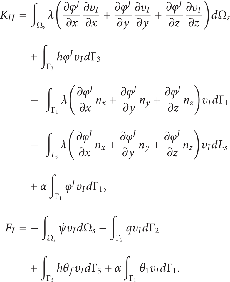
If a Heaviside step function is used as the test function for the nodes on the natural boundary or inside the domain, (11) may simplify as

3. The MLS Approximation Scheme
The MLS, originated by mathematicians for data fitting and surface construction, can be categorized as a method of finite series representation of functions. The MLS method is now a widely used alternative for constructing mesh-free shape functions for approximation.
The MLS approximation has two major features making it popular: (a) the approximated field function is continuous and smooth in the entire problem domain; (b) it is capable of producing an approximation with the desired order of consistency. The MLS approximation is described in the following.
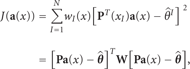
Consider a domain of definition of point x or support domain Ω x , which is located within the problem domain Ω (see Figure 2) and has a number of randomly located nodes x I (I=1,…,N). The moving least squares approximate θ h (x) of θ(x) by the following definition:

where

while the quadratic one is

The coefficient vector
where x
I
denotes the position vector of node I;w
I
(x) is the weight function associated with the node I. N is the number of nodes in Ω for which the weight functions w
I
(x)>0. The matrix


In (19),
In order to obtain the coefficient

This leads to the following set of linear relations:

where the matrixes
Solving

where Φ
T
(x) =

In practical applications, the weight function w I (x) is generally nonzero over the small neighborhood of node x I , and this neighborhood is called the domain of influence or the domain of definition (Figure 2). Typically, the shape of the domain in the two-dimensional space can be circular, elliptic, rectangular, or any other convenient regular closed line and in the three-dimensional space can be sphere, ellipsoid, cube, or any other convenient regular closed surface. In the present analysis, a spherical support domain has been selected. The choice of weight function w I (x) affects the resulting approximation θ h (x); therefore, the selection of the appropriate weight function is crucially important. The quadratic spline weight function is used in this analysis as shown to be effective in numerical practices [1, 2]. Thus we have

where d I is the distance between points x and nod x I , and r I is the size of the support domain (Figure 2). It can be seen that the quadratic spline weight function is C1 continuous over the entire domain.
4. Results of Numerical Examples
To study the accuracy and efficiency of the MLPG method, several examples are given in this section. Numerical results obtained from the present approach are compared with the exact solutions, and excellent agreement is achieved.
4.1. Illustrative Example 1
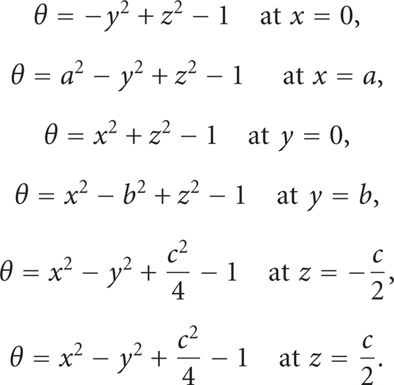
Consider the problem of the 3D heat conduction (1) with the following boundary conditions:

The exact solutions for this problem are as follows:

The geometry for this example is shown in Figure 3. The node distribution with the grid of 64 nodes is presented in Figure 4 for the case of a=b=c=1. The temperature distribution diagrams along two lines are exhibited in Figures 5 and 6.

Geometry used for example 1 (

Regular node distribution for example 1.

Temperature distribution along

Temperature distribution along
As it is observed from these figures, the MLPG results agree well with the exact solutions of the problem.
4.2. Illustrative Example 2
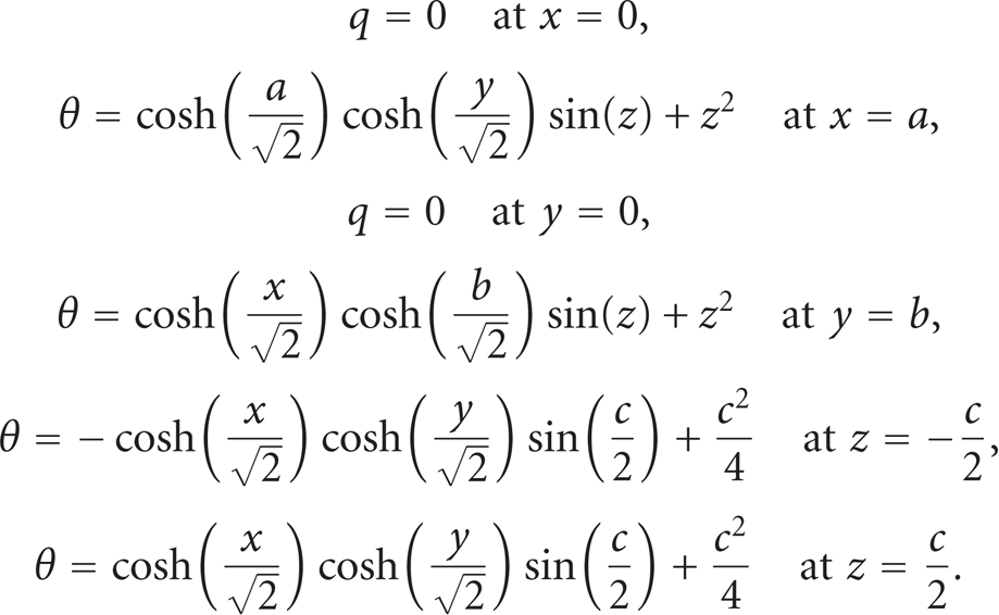
Consider the problem of the 3D heat conduction (1) with the following boundary conditions:

with the same geometry and node distribution as shown in Figures 3 and 4.
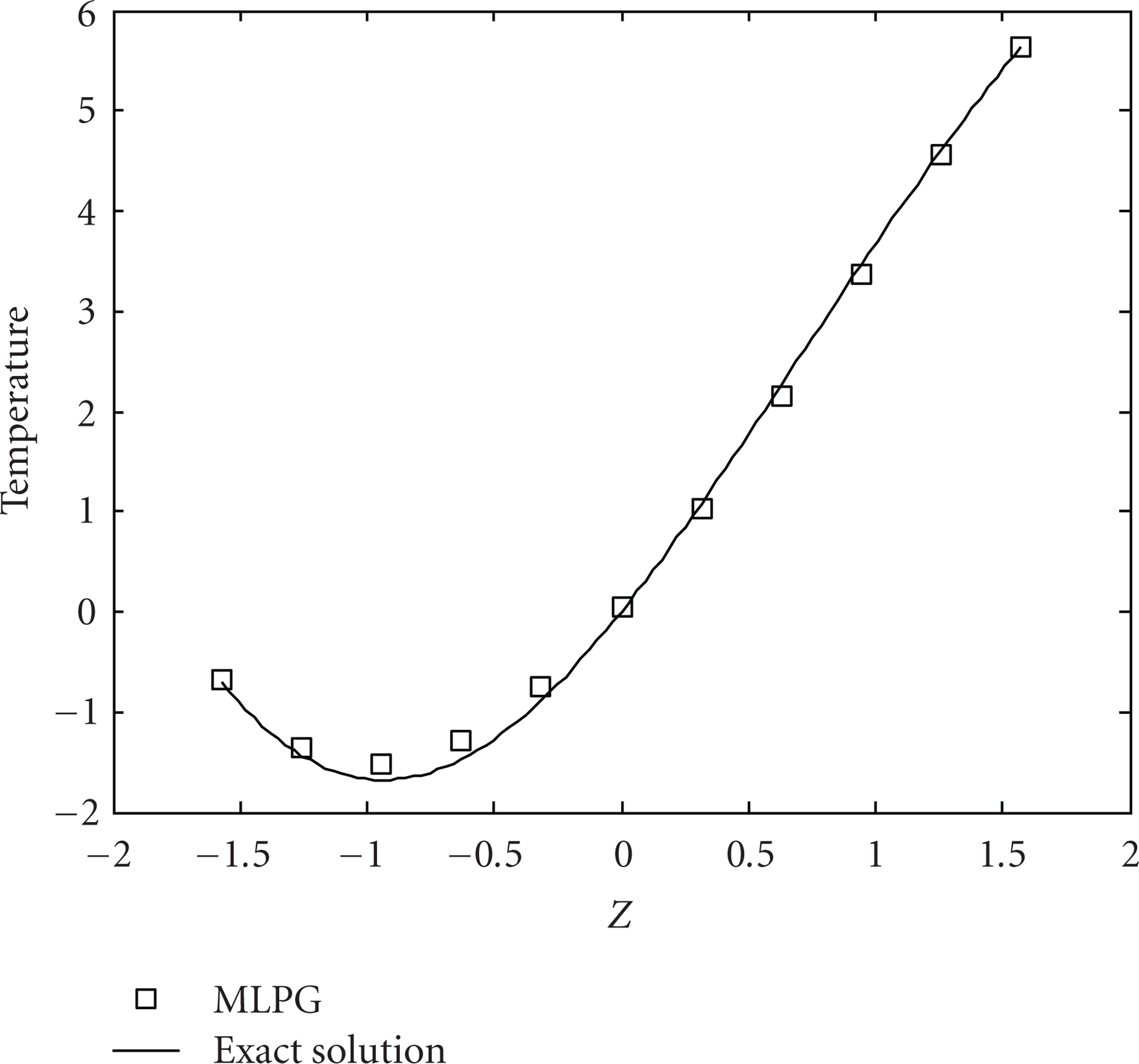
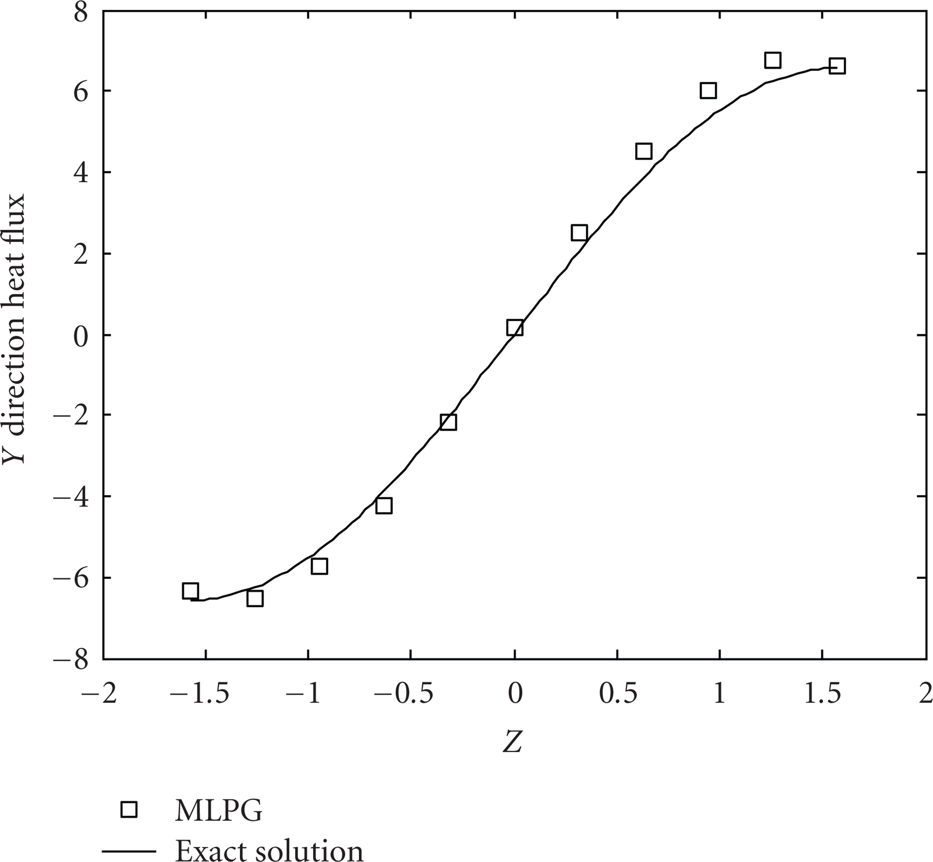
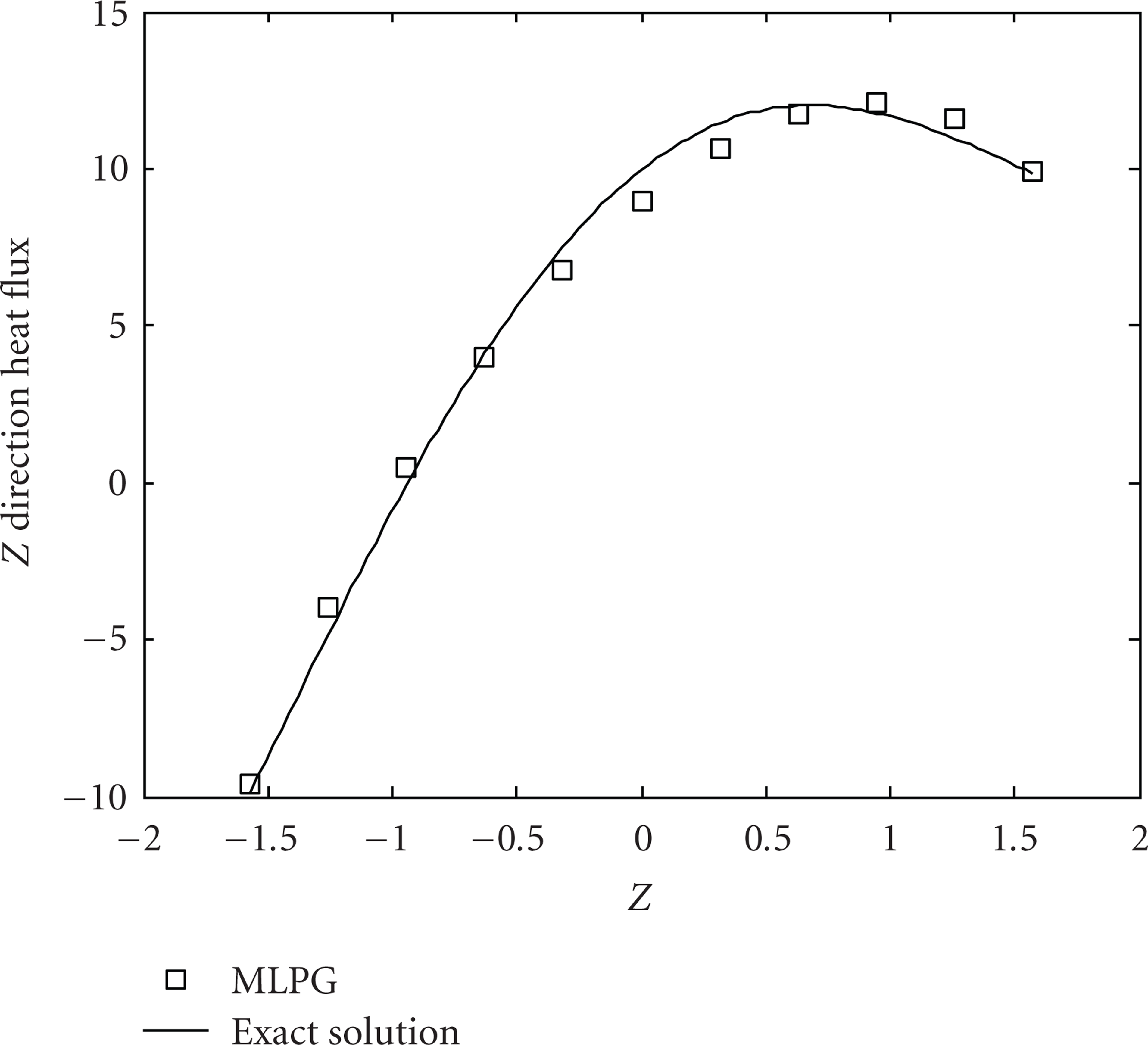
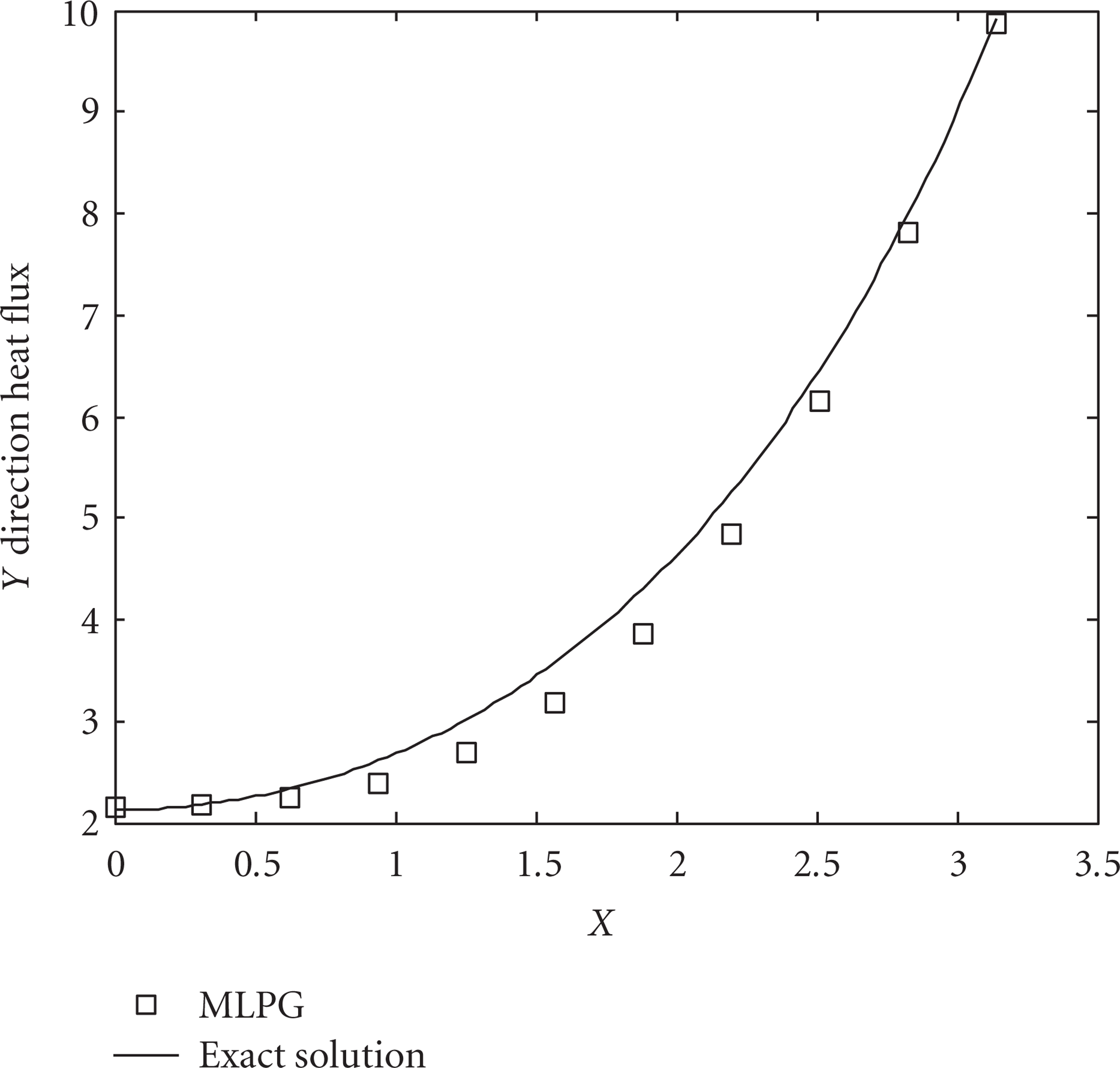
The exact solutions for this problem are

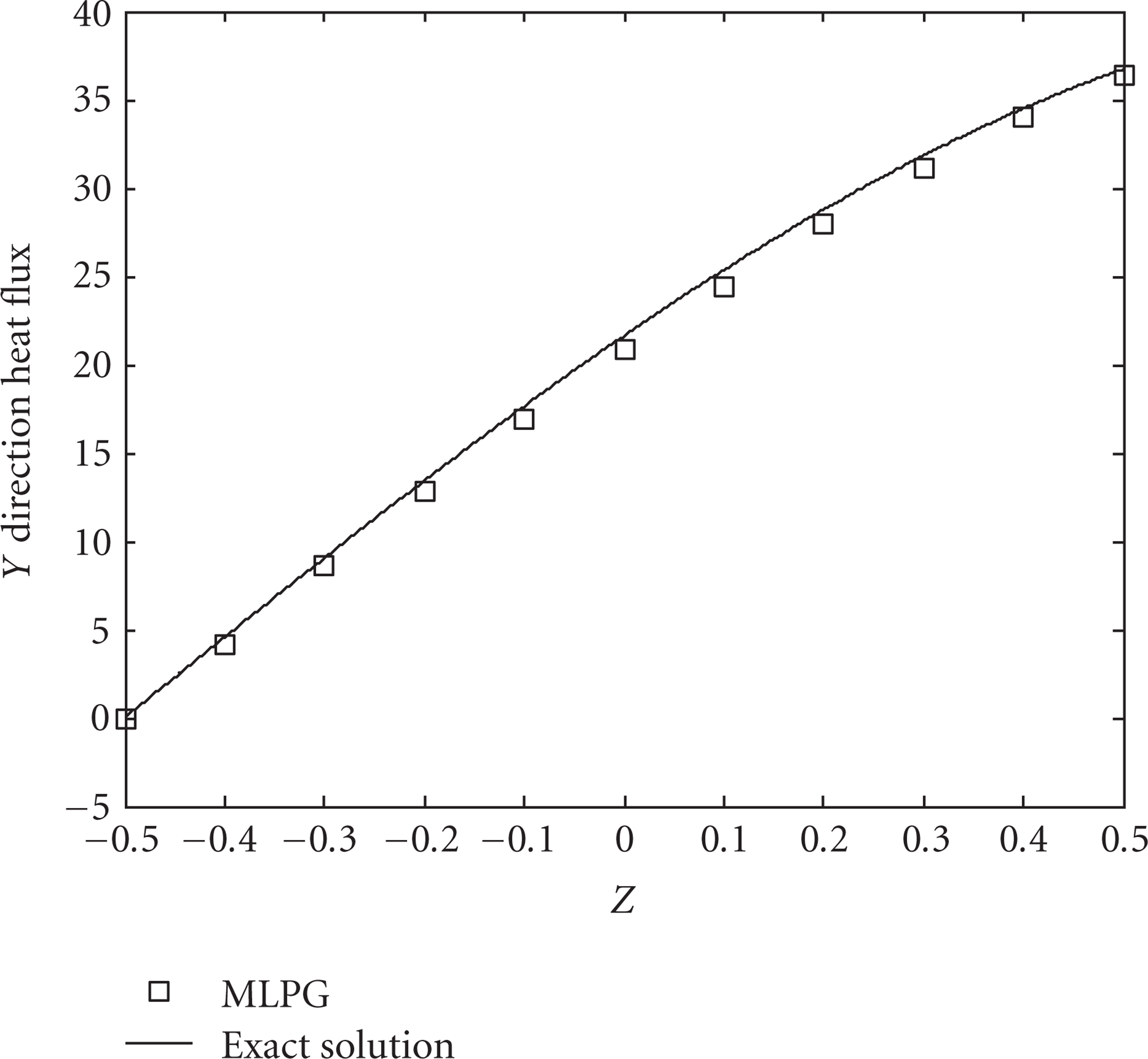
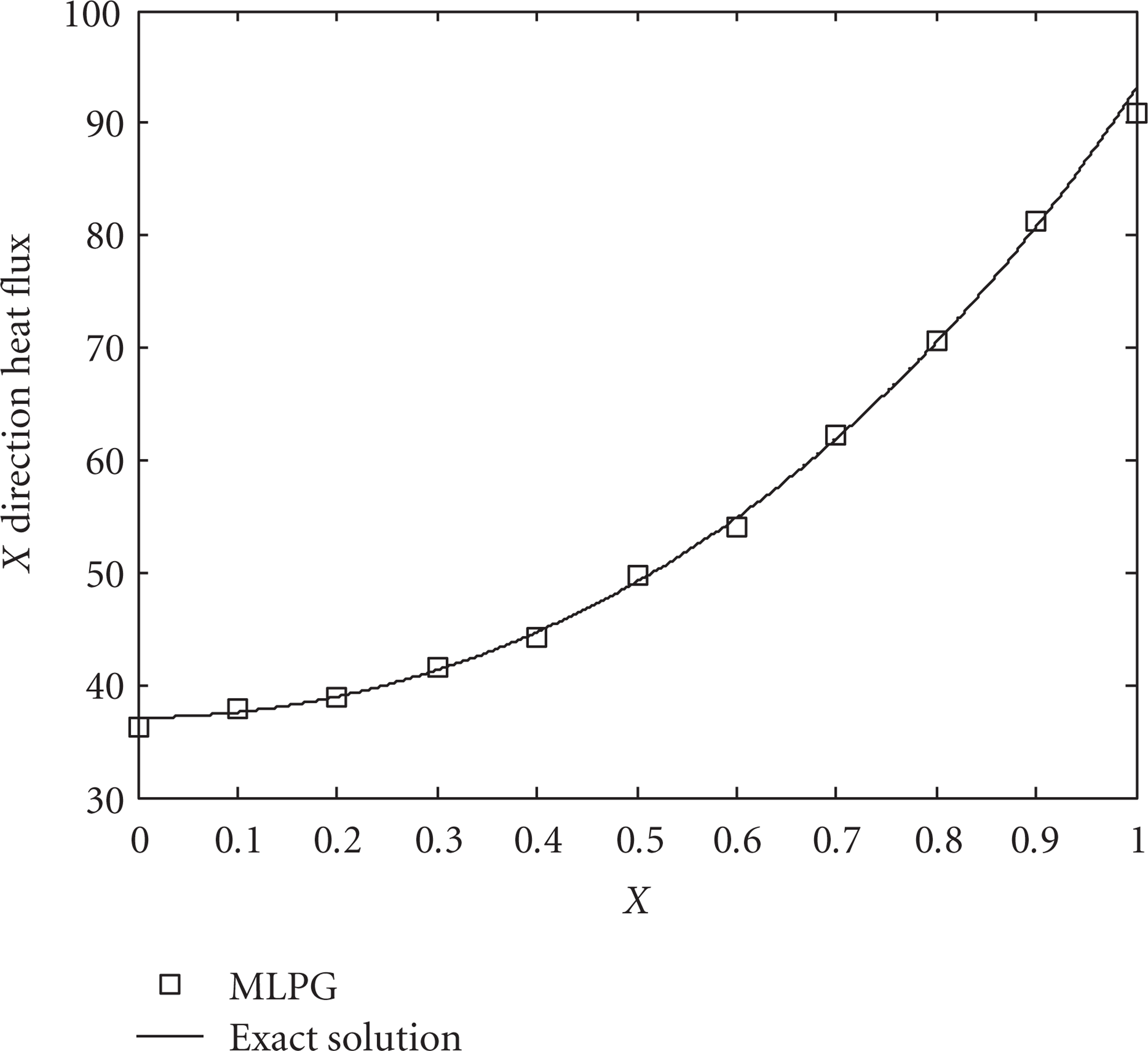
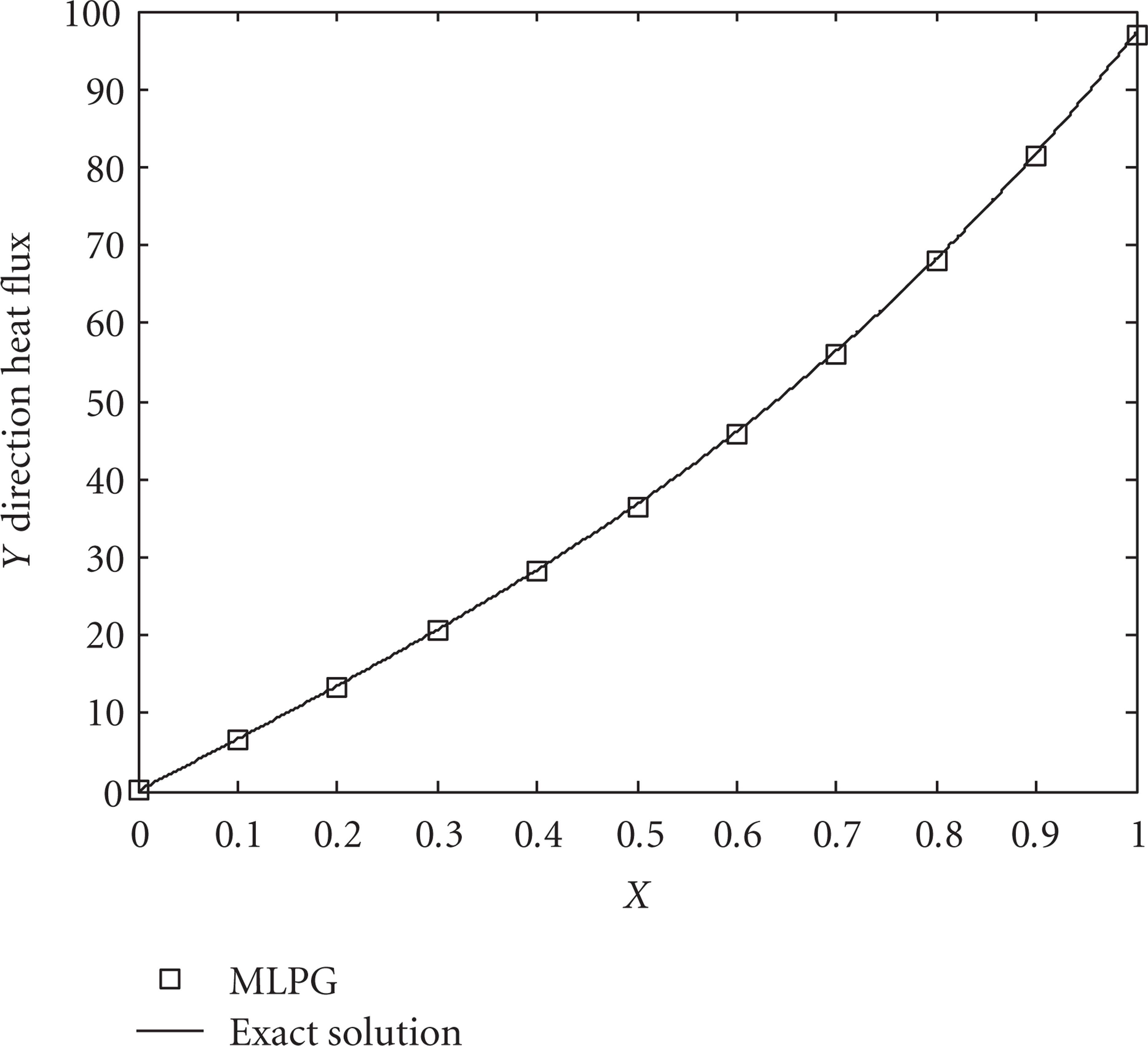
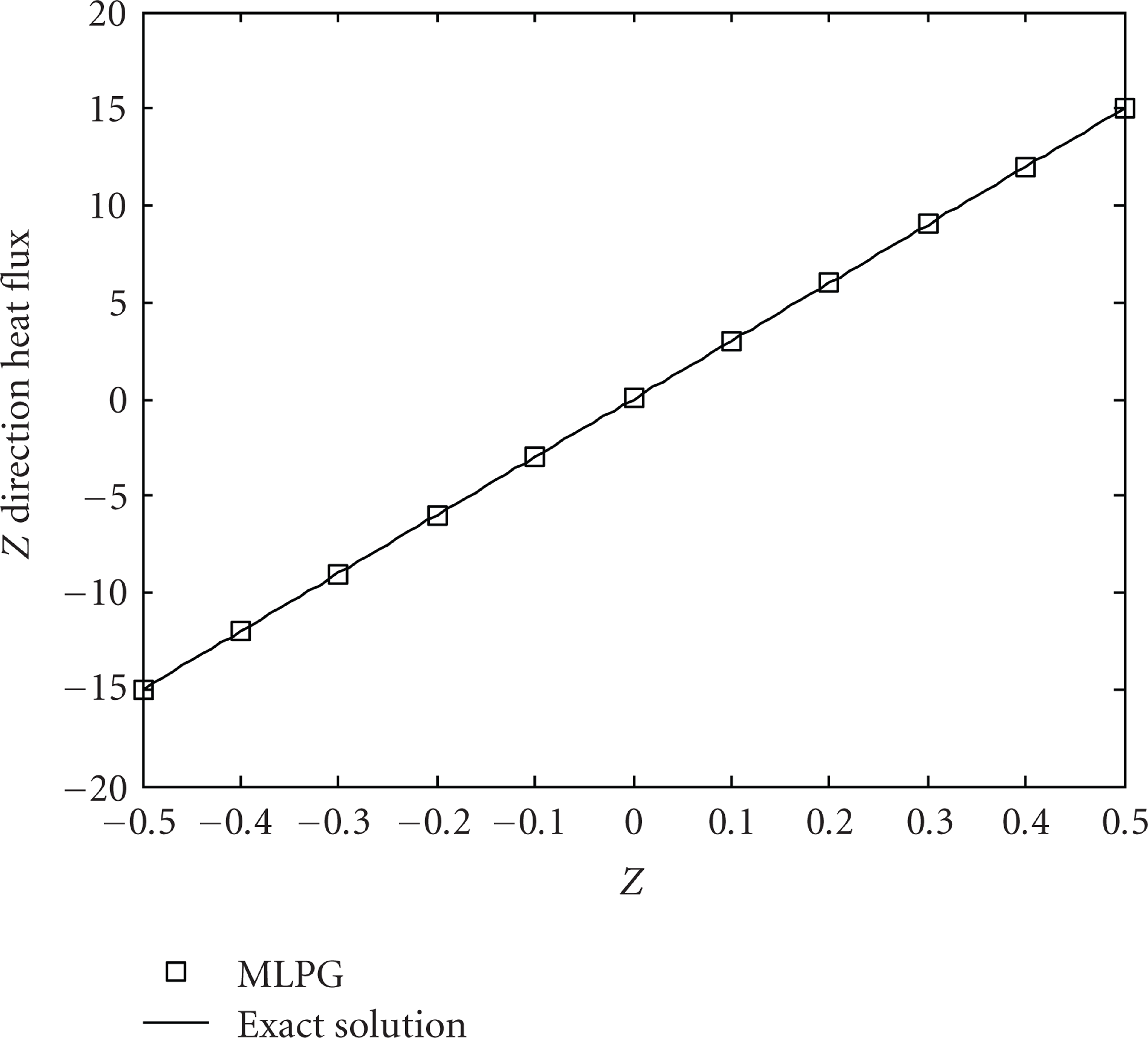
The temperature distributions and the heat flux distributions are presented in Figures 7, 8, 9, 10, 11, 12, and 13. As shown in these figures, the MLPG results admit a remarkable accuracy.

Temperature distribution along

Heat flux distribution along
Heat flux distribution along
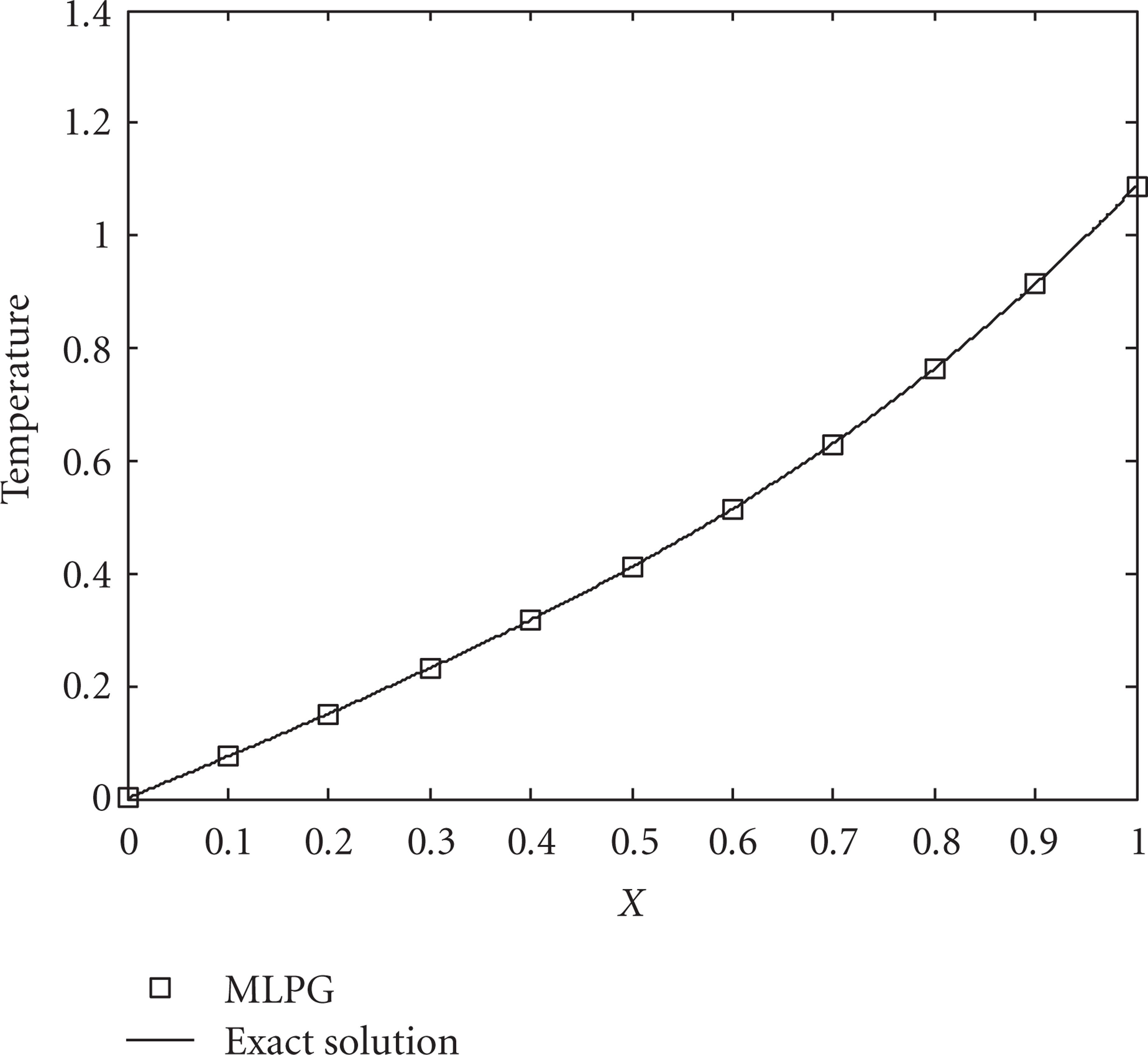
Temperature distribution along
Heat flux distribution along
Heat flux distribution along

Heat flux distribution along
4.3. Illustrative Example 3
Consider the problem of the 3D heat conduction ((1)) with the following boundary conditions:
The geometry is the same as in Figure 3 for the case of

Regular node distribution for example 3.
The exact solutions for this case are as follows:

The temperature and heat flux distributions are presented in Figures 15, 16, 17, 18, and 19. These figures show that the MLPG results agree with the exact solutions.

Temperature distribution along
Heat flux distribution along

Temperature distribution along

Heat flux distribution along

Heat flux distribution along
4.4. Illustrative Example 4
Consider the problem of the 3D heat conduction (1) with the following boundary conditions
Here, the geometry is the same as in Figure 3 for the case of

The temperature and heat flux distributions for this case are also illustrated in Figures 21, 22, 23, and 24. Once again, an excellent agreement is achieved with the exact solutions.

Regular node distribution for example 4.
Temperature distribution along
Heat flux distribution along
Heat flux distribution along
Heat flux distribution along
5. Results Comparison of MLPG and FDM
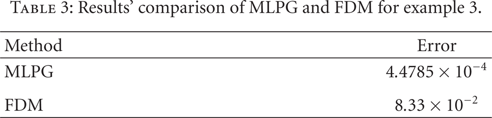
Also for comparison, the obtained results from the proposed method are illustrated with results of FDM in Tables 1, 2, 3, and 4. In these tables, errors are the error average of non-boundary nodes temperature.
Results’ comparison of MLPG and FDM for example 1.

Results’ comparison of MLPG and FDM for example 2.

Results’ comparison of MLPG and FDM for example 3.
Results’ comparison of MLPG and FDM for example 4.

It can be seen that, for example 3 and 4, the obtained results from MLPG are better than FDM; also, MLPG shows an acceptable accuracy in example 1 and 2. Nevertheless, MLPG can calculate the problem values in each desired position; however, FDM could calculate these values just in the node points.
6. Conclusion
The meshless local Petrov-Galerkin method is applied to analyze the three-dimensional steady-state heat conduction problems. Using a Heaviside test function, the domain of the integral in the weak form is simplified. This substantially reduces the computational efforts needed for constructing the stiffness matrix. Hence, the present approach is computationally efficient compared to the conventional MLPG method. The penalty approach is used to impose the essential boundary conditions, and the moving least squares approximation is used for interpolation schemes. Having established the accuracy of obtained numerical results, the efficiency as well as the capability of the present technique is clarified. Also, one of the most impotent benefits of MLPG rather than the other methods such as FDM is that MLPG can calculate the problem values in each desired position; however, FDM could calculate these values just in the node points.