Total Least Squares Method for Robust Source Localization in Sensor Networks Using TDOA Measurements

Abstract

The TDOA-based source localization problem in sensor networks is considered with sensor node location uncertainty. A total least squares (TLSs) algorithm is developed by a linear closed-form solution for this problem, and the uncertainty of the sensor location is formulated as a perturbation. The sensitivity of the TLS solution is also analyzed. Simulation results show its improved performance against the classic least squares approaches.

1. Introduction

Driven by many practical applications such as environment monitoring, traffic management in intelligent transportation, healthcare for the older and disabled, cyber-physical system (CPS) has emerged as a new advanced system to link the virtual cyber world with the real physical world [1, 2]. Sensor network is crucial to enable CPS by efficient monitoring and understanding the physical world. The main purpose of a sensor network is to monitor an area, including detecting, identifying, localizing, and tracking one or more objects of interest. These networks may be used by the military in surveillance, reconnaissance, and combat scenarios or around the perimeter of a manufacturing plant for intrusion detection. The problem of source localization involves the estimation of the position of a stationary transmitter from multiple noisy sensor measurements, which can be time-of-arrival (TOA), time-difference-of-arrival (TDOA), or angle-of-arrival (AOA) measurements or a combination of them [3–5].

Source localization methods using TDOA measurements locate the source at the intersection of a set of hyperboloids. Finding this intersection is a highly nonlinear problem [6, 7]. Over the years, many iterative numerical algorithms have been proposed for the problem, including the maximum likelihood estimation methods [8, 9] and the constrained optimization methods [10, 11]. In these approaches, linear approximation and iterative numerical techniques have to be used to deal with the nonlinearity of the hyperbolic equations. However, it is difficult to select a good initial guess to avoid a local minimum for them; therefore the convergence to the optimal solution cannot be guaranteed. The closed-form solution methods are widely used since no initial solution guesses are required and have no divergence problem compared with the iterative techniques [12–16]. For real-time application in WSNs, the iterative procedure for iterative algorithm is time consuming while the closed-form method is computational efficient.

The aforementioned approaches need the precise location of sensors. In practice, the receiver locations may not be known exactly. For example, in sensor network applications, the receivers can be with airplanes or unmanned aerial vehicles (UAVs) whose positions and velocities may not be precisely known. Hence, the inaccuracy in receiver locations needs to be taken into account in practical applications which is challenging and difficult as the estimation performance of source location can be very sensitive to the accurate knowledge of the receiver positions and a slight error in a receiver's location can lead to a big error in the source location estimate. In [17], a closed-form solution is proposed that takes the receiver error into account to reduce the estimation error. The proposed solution is computationally efficient and does not have the divergence problem as in the iterative techniques. In [18], the maximum likelihood formulation of source localization problem is given and an efficient convex relaxation for this nonconvex optimization problem is proposed. A formulation for robust source localization in the presence of sensor location errors is also proposed. Both the above methods assume that the measurement noise is Gaussian and characterize the uncertainty by stochastic approach with the perturbation being white and Gaussian.

However, such white and Gaussian assumptions are unrealistic in many practical applications [19–21]. Usually, if the Gaussian assumption are not met, the maximum-likelihood-based results under Gaussian assumption may lead to poor estimation performance, which means that the estimation performance is sensitive to the exact knowledge of the parameters of the system (see, e.g., [22]). These facts motivate us to further research on robust source localization method without any distribution assumption for measurements noise and sensor location error.

In this paper, we will develop a total least squares (TLSs) algorithm for location estimation of a stationary source. TLS is a least squares data modeling technique in which observational errors on both dependent and independent variables are taken into account. The uncertainty of the sensor location is formulated as a perturbation on the given sensor location. The sensitivity of the TLS solution will also be analyzed to show the superiority of our proposed algorithm. Compared with the existing methods which need the Gaussian assumption for both measurements noise and sensor location error, the TLS approach does not depend on any assumed distribution of the noise and errors. Simulation results support the above analysis and show good performance of the proposed method.

The rest of this paper is organized as follows. In Section 2, a linear closed-form solution is given for source localization problem using TDOA measurements. The total least squares method for source localization with sensor location uncertainty is given in Section 3, and the corresponding sensitivity analysis is derived in Section 4. Simulation results are presented in Section 5 to show the improved performance of the proposed method against the classic least squares approaches. Concluding remarks are made in Section 6.

2. A Linear Closed-Form Solution

Assume that sensor i is located at point $S_i=\{x_i,y_i,z_i\}$ . Denote the unknown source location by $S=\{x,y,z\}$ . Let c be the signal propagation speed and N the number of sensor nodes distributed in the network. A reference node, denoted as $S_0$ , exists in the field. We define the distance from the source to sensor i as $D_i$ . The TDOA that we derive from the data, ${\tau }_{0i}$ , for each sensor node $i\in [1,N]$ relative to the reference sensor $S_0$ is

$\begin{array}{c}{\tau }_{0i}=\frac{1}{c}\Vert S-S_0\Vert -\frac{1}{c}\Vert S-S_i\Vert =\frac{1}{c}\left(D_0-D_i\right).\end{array}$

(1)

Denote the distance difference of arrival (DDOA) data for the ith sensor as

$\begin{array}{c}{d}_{0i}={\tau }_{0i}\times c=D_0-D_i.\end{array}$

(2)

We have

$\begin{array}{cc}\hfill D_0^2-D_i^2& ={\Vert S-S_0\Vert }^2-{\Vert S-S_i\Vert }^2,\hfill \\ \hfill & ={\left(x-x_0\right)}^2+{\left(y-y_0\right)}^2+{\left(z-z_0\right)}^2,\hfill \\ \hfill & \hspace{1em}-\left({\left(x-x_i\right)}^2+{\left(y-y_i\right)}^2+{\left(z-z_i\right)}^2\right),\hfill \\ \hfill & =x_0^2-x_i^2+2x\left(x_i-x_0\right)+y_0^2-y_i^2+2y\left(y_i-y_0\right),\hfill \\ \hfill & \hspace{1em}+z_0^2-z_i^2+2z\left(z_i-z_0\right),\hfill \\ \hfill & =D_0^2-{\left(D_0-d_{0i}\right)}^2,\hfill \\ \hfill & =2D_0{d}_{0i}-d_{0i}^2.\hfill \end{array}$

(3)

Group all the known terms together and denote

$\begin{array}{c}{b}_i=\frac{1}{2}\left[x_0^2-x_i^2+y_0^2-y_i^2+z_0^2-z_i^2+d_{0i}^2\right]\end{array}.$

(4)

Rearranging and substituting give

$\begin{array}{c}\left(x_0-x_i\right)x+\left(y_0-y_i\right)y+\left(z_0-z_i\right)z+d_{0i}{D}_0=b_i,\end{array}$

(5)

which is a linear model for unknown parameters $x,y,z$ , and   $D_0$ . Stacking the N sensor measurements, we have the linear system in matrix form

$\begin{array}{c}AX=b,\end{array}$

(6)

where

$\begin{array}{c}A=\left[\begin{array}{cccc}{x}_0-x_1& y_0-y_1& z_0-z_1& d_{01}\\ x_0-x_2& y_0-y_2& z_0-z_2& d_{02}\\ ⋮& ⋮& ⋮& ⋮\\ x_0-x_N& y_0-y_N& z_0-z_N& d_{0N}\end{array}\right],\\ X=\left[\begin{array}{c}x\\ y\\ z\\ D_0\end{array}\right],\hspace{1em}\hspace{1em}b=\left[\begin{array}{c}{b}_1\\ b_2\\ ⋮\\ b_N\end{array}\right].\end{array}$

(7)

When the location of sensor nodes can be precisely known and the TDOA measurements are noise-free, linear system (6) is compatible. The solution is unique while the data matrix A is of full rank.

In [16], a noise ɛ is considered at the right side of (6):

$\begin{array}{c}AX=b+\varepsilon .\end{array}$

(8)

The least squares (LSs) problem seeks to

$\begin{array}{cc}\hfill & \text{minimize}:\hspace{1em}\Vert b-b_{\text{ls}}\Vert ,\hfill \\ \hfill & \text{subject}\hspace{0.17em}\hspace{0.17em}\text{to}:\hspace{1em}{b}_{\text{ls}}\in \mathcal{R}\left(A\right),\hfill \end{array}$

(9)

where $ℛ(A)$ denote the vector space spanned by the column vector of matrix A. Once a minimizing $b_{\text{ls}}$ is found, then any X satisfying $AX=b_{\text{ls}}$ is called an LS solution and $b-b_{\text{ls}}$ the corresponding LS correction. The unique LS solution can be obtained while the data matrix A is of full rank:

$\begin{array}{c}{X}_{\text{ls}}={\left(A^{T}A\right)}^{-1}{A}^{T}b.\end{array}$

(10)

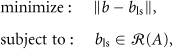
The ordinary LS problem amounts to perturbing the observation vector b by a minimum amount $b-A{X}_{ls}$ . The underlying assumption is that errors only occur in the vector b and that the matrix A is exactly known. However, the TDOA measurements always have noise, that is, $d_{0i}$ is perturbed by a noise. Hence, both sides of (5) have perturbation according to term $d_{0i}$ . Besides, in practice, the receiver locations may not be known exactly. As a result, the inaccuracy in receiver locations needs to be taken into account in practical environments. Therefore, considering only the perturbation at the right side of (6) is not enough. We should consider the perturbations at both sides.

3. Total Least Squares Solution

The definition of the total least squares method is motivated by the asymmetry of the least squares method that b is corrected while A is not. Provided that both A and b are given data, it is reasonable to treat them symmetrically. One important application of TLS problem is parameter estimation in errors-in-variables models, that is, considering the measurements in A [23, 24]. We assume that the m measurement in $\tilde{A}$ and $\tilde{b}$ by

$\begin{array}{c}\tilde{A}X=\tilde{b},\end{array}$

(11)

where $\tilde{A}=A+\mathrm{\Delta }A$ , $\tilde{b}=b+\mathrm{\Delta }b$ , and $AX=b$ , is compatible. The total least squares (TLSs) problem seeks to

$\begin{array}{cc}\hfill & \text{minimize}:\hspace{1em}{\Vert [\tilde{A};\tilde{b}]-\left[A_{\text{tls}};b_{\text{tls}}\right]\Vert }_F,\hfill \\ \hfill & \text{subject}\hspace{0.17em}\hspace{0.17em}\text{to}:\hspace{1em}{b}_{\text{tls}}\in \mathcal{R}\left(A_{\text{tls}}\right),\hfill \end{array}$

(12)

where ${\parallel ·\parallel }_F$ denotes the Frobenius norm of matrix A, that is,

$\begin{array}{c}{\Vert A\Vert }_F=\sqrt{{\displaystyle \sum }_{i=1}^m\hspace{0.17em}{\displaystyle \sum }_j^n{\left|a_{ij}\right|}^2}=\sqrt{\text{trace}\left(A^{T}A\right)}.\end{array}$

(13)

Once a minimizing $[A_{\text{tls}};b_{\text{tls}}]$ is found, then any X satisfying $A_{\text{tls}}X=b_{\text{tls}}$ is called a TLS solution and $[\tilde{A};\tilde{b}]-[A_{\text{tls}};b_{\text{tls}}]$ the corresponding TLS correction [25].

When A is of full rank, the closed-form expression of the basic TLS solution can be obtained as the following:

$\begin{array}{c}{X}_{\text{tls}}={\left({\tilde{A}}^T\tilde{A}-{\sigma }_{n+1}^{2}I\right)}^{-1}{\tilde{A}}^T\tilde{b},\end{array}$

(14)

where ${\sigma }_{n+1}$ is the smallest singular value of $[A;b]$ . It can be proved that the TLS solution $X_{\text{tls}}$ estimates the true parameter $A^{+}b$ consistently, that is, X_tls converges to the solution of $AX=b$ as the number of measurements tends to infinity, where $A^{+}$ denotes the Moore-Penrose pseudoinverse of matrix A. This property of TLS estimates does not depend on any assumed distribution of the errors. Note that the LS estimates are inconsistent in this case.

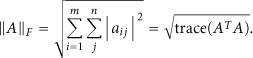
In the following, the algorithm computation complexity is analyzed by considering the number of floating-point operations (FLOPS). The calculation of FLOPS is briefly described as follows: additions and multiplications count as one FLOP each. Adding matrices of sizes $m\times n$ requires $mn$ FLOPS. Multiplying matrices of sizes $m\times k$ and $k\times p$ requires $mnk$ FLOPS. Matrix inverse of size $n\times n$ requires $n^3$ FLOPS. Singular value decomposition of matrix with size $n\times m$ requires $n{m}^2$ FLOPS. The computation overhead of three closed-form algorithms is investigated, that is, least squares (LSs) method in [16], two-stage weighted least squares (WLSs) method in [17] and the proposed TLS method. For N-deployed nodes and p dimension of source location parameter, the numbers of FLOPS in the LS, WLS, and the proposed TLS algorithms are $(2p+3)(p+1)N+{(p+1)}^3$ , $(2p+3)(2p+2)N+2{(p+1)}^3$ , and $(2p+5)(p+2)N+{(p+2)}^2(p+3)$ , respectively. It is to show that LS method is the most computationally efficient, whereas WLS method is two-stage least square and TLS method has singular value decomposition for matrix. It is clear that they all have comparable computation complexity $𝒪(N)$ since $p=3$ or $p=4$ for source localization problem.

4. Sensitivity Properties of the Solution

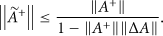
In this section, we will first examine how perturbations in A and b affect the solution X. In this analysis the condition number of the matrix A plays a significant role. The following definition generalizes the condition number of a square nonsingular matrix [26].

Definition 1.

Let $A\in {ℛ}^{m\times n}$ have rank r. The condition number of A is

$\begin{array}{c}\kappa \left(A\right)=\Vert A\Vert \cdot \Vert A^{+}\Vert =\frac{{\sigma }_1}{{\sigma }_r},\end{array}$

(15)

where ${\sigma }_1,{\sigma }_2,\dots ,{\sigma }_r$ are the singular values of A by decreasing order.

Matrices with small condition numbers are said to be well conditioned while the ones with large condition numbers are said to be ill-conditioned. Analyzing the effect of perturbation on the solution of linear system $AX=b$ , we introduce the following lemma [27].

Lemma 1.

If $\mathrm{rank}\hspace{0.17em}(\tilde{A})=\mathrm{rank}\hspace{0.17em}(A)$ and $\parallel \mathrm{\Delta }A\parallel \parallel A^{+}\parallel <1$ , then

$\begin{array}{c}\Vert {\tilde{A}}^{+}\Vert \le \frac{\Vert A^{+}\Vert }{1-\Vert A^{+}\Vert \Vert \Delta A\Vert }.\end{array}$

(16)

Theorem 1.

Denote $X_{\text{ls}}=A^{+}b$ as the LS solution of unperturbed system $AX=b$ , and ${\tilde{X}}_{\text{ls}}={\tilde{A}}^{+}\tilde{b}$ is the LS solution of perturbed system $\tilde{A}X=\tilde{b}$ with $\tilde{A}=A+\mathrm{\Delta }A$ , $\tilde{b}=b+\mathrm{\Delta }b$ . One further assumes that $\parallel \mathrm{\Delta }A\parallel \le \varepsilon \parallel A\parallel$ , $\parallel \mathrm{\Delta }b\parallel \le \varepsilon \parallel b\parallel$ , $\kappa (A)=\kappa$ . Then, one has

$\begin{array}{c}\frac{\Vert {\tilde{X}}_{\text{ls}}-X_{\text{ls}}\Vert }{\Vert X_{\text{ls}}\Vert }=\mathcal{O}\left(\varepsilon \kappa \right).\end{array}$

(17)

Proof.

Noting that A and $\tilde{A}$ are full rank and $(I-A{A}^{+})b=0$ since $b\in ℛ(A)$ , we have

$\begin{array}{cc}\hfill {\tilde{X}}_{\text{ls}}-X_{\text{ls}}& ={\tilde{A}}^{+}\tilde{b}-A^{+}b\hfill \\ \hfill & ={\tilde{A}}^{+}\left(b+\Delta b\right)-A^{+}b\hfill \\ \hfill & ={\tilde{A}}^{+}\Delta b+\left({\tilde{A}}^{+}-A^{+}\right)b\hfill \\ \hfill & ={\tilde{A}}^{+}\Delta b+\left({\tilde{A}}^{+}+{\tilde{A}}^{+}A{A}^{+}-{\tilde{A}}^{+}A{A}^{+}-A^{+}\right)b\hfill \\ \hfill & ={\tilde{A}}^{+}\Delta b+\left({\tilde{A}}^{+}+{\tilde{A}}^{+}A{A}^{+}-{\tilde{A}}^{+}A{A}^{+}-{\tilde{A}}^{+}\tilde{A}{A}^{+}\right)b\hfill \\ \hfill & ={\tilde{A}}^{+}\Delta b+{\tilde{A}}^{+}\left(I-A{A}^{+}\right)b-{\tilde{A}}^{+}\left(\tilde{A}-A\right)A^{+}b\hfill \\ \hfill & ={\tilde{A}}^{+}\Delta b-{\tilde{A}}^{+}\Delta A{X}_{\text{ls}}.\hfill \end{array}$

(18)

Therefore, $\parallel {\tilde{X}}_{\text{ls}}-X_{\text{ls}}\parallel =\parallel {\tilde{A}}^{+}\mathrm{\Delta }b-{\tilde{A}}^{+}\mathrm{\Delta }A{X}_{\text{ls}}\parallel$ . Dividing by $\parallel X_{\text{ls}}\parallel$ at both sides, we have

$\begin{array}{cc}\hfill \frac{\Vert {\tilde{X}}_{\text{ls}}-X_{\text{ls}}\Vert }{\Vert X_{\text{ls}}\Vert }& =\frac{\Vert {\tilde{A}}^{+}\Delta b-{\tilde{\text{A}}}^{+}\Delta A{X}_{\text{ls}}\Vert }{\Vert X_{\text{ls}}\Vert }\hfill \\ \hfill & \le \frac{{\tilde{A}}^{+}\Delta b}{\Vert X_{\text{ls}}\Vert }+\Vert {\tilde{A}}^{+}\Delta A\Vert \hfill \\ \hfill & \le \Vert {\tilde{A}}^{+}\Vert \left(\frac{\Vert \Delta b\Vert }{\Vert X_{\text{ls}}\Vert }+\Vert \Delta A\Vert \right)\hfill \\ \hfill & \le \Vert {\tilde{A}}^{+}\Vert \left(\frac{\varepsilon \Vert b\Vert }{\Vert X_{\text{ls}}\Vert }+\varepsilon \Vert A\Vert \right)\hfill \\ \hfill & \le \frac{\Vert A^{+}\Vert }{1-\Vert A^{+}\Vert \Vert \Delta A\Vert }\left(\frac{\varepsilon \Vert b\Vert }{\Vert X_{\text{ls}}\Vert }+\varepsilon \Vert A\Vert \right)\hfill \\ \hfill & \le \frac{\Vert A^{+}\Vert }{1-\Vert A^{+}\Vert \varepsilon \Vert A\Vert }\left(\frac{\varepsilon \Vert b\Vert }{\Vert X_{\text{ls}}\Vert }+\varepsilon \Vert A\Vert \right)\hfill \\ \hfill & =\frac{1}{1-\varepsilon \kappa }\left(\frac{\varepsilon \Vert A^{+}\Vert \Vert b\Vert }{\Vert A^{+}b\Vert }+\varepsilon \kappa \right)\hfill \\ \hfill & =\frac{1}{1-\varepsilon \kappa }\left(\frac{\varepsilon \Vert A^{+}\Vert \Vert A{A}^{+}b\Vert }{\Vert A^{+}b\Vert }+\varepsilon \kappa \right)\hfill \\ \hfill & \le \frac{1}{1-\varepsilon \kappa }\left(\frac{\varepsilon \Vert A^{+}\Vert \Vert A\Vert \Vert A^{+}b\Vert }{\Vert A^{+}b\Vert }+\varepsilon \kappa \right)\hfill \\ \hfill & =\frac{2\varepsilon \kappa }{1-\varepsilon \kappa }=\mathcal{O}\left(\varepsilon \kappa \right).\hfill \end{array}$

(19)

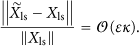
From the theorem we can see that, only when the perturbations are sufficiently small, the LS solution is a good estimator of the true solution of $AX=b$ .

Additionally, we will show when the TLS solution has better performance than the LS solution for the perturbed model $\tilde{A}X\approx \tilde{b}$ . Denote the singular value decomposition (SVD) of A by

$\begin{array}{c}A=U\Sigma V^T,\end{array}$

(20)

where

$\begin{array}{cc}\hfill U& =\left[u_1,u_2^{\prime },\dots ,u_m\right],\hspace{1em}{U}^{\prime }\in {\mathcal{R}}^m,\hspace{0.17em}\hspace{0.17em}{U}^{T}U=I_m,\hfill \\ \hfill V& =\left[v_1,v_2^{\prime },\dots ,v_n\right],\hspace{1em}{V}^{\prime }\in {\mathcal{R}}^n,\hspace{0.17em}\hspace{0.17em}{V}^T\text{V}=I_n,\hfill \\ \hfill \Sigma & =\mathrm{diag}\left({\sigma }_1,{\sigma }_2,\dots ,{\sigma }_n\right)\in {\mathcal{R}}^{m\times n},\hspace{1em}{\sigma }_1\ge {\sigma }_2\ge \cdots \ge {\sigma }_n\ge 0,\hfill \end{array}$

(21)

denote the singular value decomposition (SVD) of $\tilde{A}$ by

$\begin{array}{c}A+\Delta A=\tilde{A}=U^{\prime }{\Sigma }^{\prime }{V}^{\prime T},\end{array}$

(22)

where

$\begin{array}{cc}\hfill U\prime & =\left[u_1^{\prime },u_2^{\prime },\dots ,u_m^{\prime }\right],\hspace{1em}{U}^{\prime }\in {\mathcal{R}}^m,\hspace{0.17em}\hspace{0.17em}{U^{\prime }}^T{U}^{\prime }=I_m,\hfill \\ \hfill V\prime & =\left[v_1^{\prime },v_2^{\prime },\dots ,v_n^{\prime }\right],\hspace{1em}{V}^{\prime }\in {\mathcal{R}}^n,\hspace{0.17em}\hspace{0.17em}{V^{\prime }}^T{V}^{\prime }=I_n,\hfill \\ \hfill \Sigma \prime & =\mathrm{diag}\left({\sigma }_1^{\prime },{\sigma }_2^{\prime },\dots ,{\sigma }_n^{\prime }\right)\in {\mathcal{R}}^{m\times n},\hfill \\ \hfill & \hspace{1em}\hspace{1em}\hspace{1em}\hspace{1em}{\sigma }_1^{\prime }\ge {\sigma }_2^{\prime }\ge \dots \ge {\sigma }_n^{\prime }\ge 0,\hfill \end{array}$

(23)

and denote the SVD of $[\tilde{A};\tilde{b}]$ by

$\begin{array}{c}\left[A+\Delta A;b+\Delta b,\tilde{A};\tilde{b}\right]=\tilde{U}\tilde{\Sigma }{\tilde{V}}^T,\end{array}$

(24)

where

$\begin{array}{cc}\hfill \tilde{U}& =\left[{\tilde{u}}_1,{\tilde{u}}_2,\dots ,{\tilde{u}}_m\right],\hspace{1em}\tilde{U}\in {\mathcal{R}}^m,\hspace{0.17em}\hspace{0.17em}{\tilde{U}}^T\tilde{U}=I_m,\hfill \\ \hfill \tilde{V}& =\left[{\tilde{v}}_1,{\tilde{v}}_2,\dots ,{\tilde{v}}_n\right],\hspace{1em}\tilde{V}\in {\mathcal{R}}^{\left(n+1\right)},\hspace{0.17em}\hspace{0.17em}{\tilde{V}}^T\tilde{V}=I_{n+1},\hfill \\ \hfill \tilde{\Sigma }& =\mathrm{diag}\left({\tilde{\sigma }}_1,{\tilde{\sigma }}_2,\dots ,{\tilde{\sigma }}_n,{\tilde{\sigma }}_{n+1}\right)\in {\mathcal{R}}^{m\times n+1},\hfill \\ \hfill & \hspace{1em}\hspace{1em}\hspace{1em}\hspace{1em}\hspace{0.17em}{\tilde{\sigma }}_1\ge {\tilde{\sigma }}_2\ge \cdots \ge {\tilde{\sigma }}_{(n+1)}\ge 0.\hfill \end{array}$

(25)

The accuracy of TLS and LS solutions related to the perturbation effects on singular values and associated singular subspaces [23]. Several papers have analyzed the bounds on the perturbation effects related to singular subspaces [28–30]. The most interesting results for sensitivity analysis of TLS solution are given in [30].

Definition 2.

Denote two subspaces as L and M. For any unitary invariant norm, the distance between two subspaces is defined as the sine of the largest canonical angle

$\begin{array}{c}\mathrm{dist}\left(L,M\right)=\Vert \sin \Theta \left(L,M\right)\Vert =\Vert \left(I-P_M\right)P_L\Vert ,\end{array}$

(26)

where $P_M$ and $P_L$ are the projection operators [29, 30].

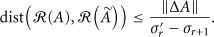
Theorem 2.

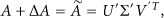
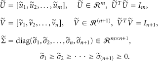
Let the SVD of $A\in {ℛ}^{m\times n},m\ge n$ , be given by (20), $\mathrm{rank}\hspace{0.17em}(A)=r$ . Add perturbations $\mathrm{\Delta }A$ to A, and let SVD of $\tilde{A}$ be given by (22). If ${\sigma }_r^{\prime }-{\sigma }_{r+1}>0$ , then

$\begin{array}{c}\mathrm{dist}\left(\mathcal{R}\left(A\right),\mathcal{R}\left(\tilde{A}\right)\right)\le \frac{\Vert \Delta A\Vert }{{\sigma }_r^{\prime }-{\sigma }_{r+1}}.\end{array}$

(27)

Theorem 2 is a special case of the generalized $\sin \theta$ -theorem in [30].

Recall the perturbed system $\tilde{A}X\approx \tilde{b}$ ; LS projects $\tilde{A}$ and $\tilde{b}$ into the singular subspaces

$\begin{array}{c}\mathcal{L}\left(u_1^{\prime },u_2^{\prime },\dots ,u_m^{\prime }\right)=\mathcal{R}\left(\tilde{A}\right),\end{array}$

(28)

while the TLS projects $\tilde{A}$ and $\tilde{b}$ into the singular subspaces

$\begin{array}{c}\mathcal{L}\left({\tilde{u}}_1,{\tilde{u}}_2,\dots ,{\tilde{u}}_m\right)=\mathcal{R}\left(\left[\tilde{A};\tilde{b}\right]\right).\end{array}$

(29)

Furthermore, the real source location $X\in ℛ(A)$ , since $AX=b$ . Therefore, it is important to analyze the distance between $ℛ(\tilde{A})$ , $ℛ([\tilde{A};\tilde{b}])$ and $ℛ(A)$ . Assumeing that A and $\tilde{A}$ have full rank, we can obtain the following corollary according to Theorem 2.

Corollary 1.

One has

$\begin{array}{c}\mathrm{dist}\left(\mathcal{R}\left(A\right),\mathcal{R}\left(\tilde{A}\right)\right)\le \frac{\Vert \Delta A\Vert }{{\sigma }_n^{\prime }},\\ \mathrm{dist}(\mathcal{R}\left(A\right),\mathcal{R}\left(\left[\tilde{A};\tilde{b}\right]\right)\phantom{\left[\tilde{A};\tilde{b}\right]})\le \frac{\Vert \Delta A\Vert }{{\tilde{\sigma }}_n}.\end{array}\begin{array}{c}\end{array}$

(30)

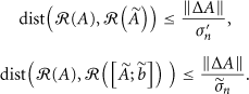
The interlacing theorem (see [31]) implies that

$\begin{array}{c}{\sigma }_1^{\prime }\ge {\tilde{\sigma }}_1\ge \cdots \ge {\sigma }_n^{\prime }\ge {\tilde{\sigma }}_n.\end{array}$

(31)

Therefore,

$\begin{array}{c}\frac{\Vert \Delta A\Vert }{{\tilde{\sigma }}_n}\le \frac{\Vert \Delta A\Vert }{{\sigma }_n^{\prime }}.\end{array}$

(32)

From Corollary 1 we can see that the upper bound of the distance between $ℛ(\tilde{A})$ and $ℛ(A)$ is smaller than the upper bound of distance between $ℛ([\tilde{A};\tilde{b}])$ and $ℛ(A)$ . This implies that the TLS solution is expected to be closer to its corresponding unperturbed subspace. Hence, the TLS solution is expected to be more accurate than the LS solution.

5. Simulations

5.1. Simulation Setup

In this section, simulations are carried out to show the effectiveness of the proposed method. Two scenarios are investigated for their effects on localization performance, including Gaussian distribution and truncated Gaussian distribution for measurement noise and sensor node location error. In our simulation, unless otherwise specified, sensors are randomly deployed in a $5000\hspace{0.17em}\text{m}\times 5000\hspace{0.17em}\text{m}$ area with uniform distribution. An example is shown in Figure 1, where 30 nodes are uniformly distributed. The source is denoted as a triangle with red and the reference node is denoted as a square in blue. The exact location of the reference node can be known.

Figure 1

Simulation scenario.

In order to show the improved performance of our proposed method with the existing closed-form method, we investigate LS method in [16] and WLS method in [17]. Root mean square error (RMSE) is used as the criterion for localization performance. The following simulations are performed with 500 Monte Carlo trials. In all figures, the red solid line with square, black dash line with circle, and blue dotted dash line with triangle represent the results of TLS, WLS, and LS solutions, respectively.

5.2. Gaussian Case

In this case, we consider the Gaussian distribution for both measurement noise and sensor node location error. The effect on estimation performance for different measurement noise variance value is investigated. Measurement noise variance $({\sigma }_n)$ is changed in the range 10–100. The variance of perturbation $({\sigma }_p)$ is set to be a constant number 25. The localization performance variation with noise variance is depicted in Figure 2. As noise variance increases, localization performance degrades in all LS, WLS, and TLS algorithms. The TLS algorithm outperforms the LS and WLS algorithms.

Figure 2

Localization errors versus noise variance (Gaussian case).

In the second simulation, the effect on estimation performance with different variance of perturbation is investigated. The variance of perturbation is set to be varied from 10 to 100 and sensors are deployed uniformly. The measurement noise variance is set to be 50. The localization performance variation with variance of perturbation is depicted in Figure 3. The TLS algorithm outperforms the LS and WLS significantly with high-level variance of perturbation.

Figure 3

Localization errors versus perturbation variance (Gaussian case).

The estimation performance of three algorithms is also investigated with different numbers of deployed nodes. Figure 4 shows the RMSEs versus the number of nodes. Fifty nodes are uniformly generated in the field. Localization starts by using five randomly selected nodes for each algorithm, followed by adding more nodes of five in a group until all fifty nodes are used. The number of FLOPS is considered to evaluate the algorithm computational complexity with variation of the number of nodes. Results are given in Figure 5 with 2-dimensional source location parameter and 5–50 nodes. It can be seen that LS required the fewest FLOPS while TLS required the most FLOPS with SVD of matrix. Although the estimation performance is improved with more nodes for all algorithms, the computation overhead is also increased. t is to show that LS method is the most computationally efficient, whereas WLS method is two-stage least square method and TLS method has singular value decomposition for matrix.

Figure 4

Localization errors versus number of nodes (Gaussian case).

Figure 5

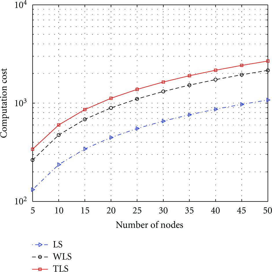
Computation cost versus number of nodes.

5.3. Truncated Gaussian Case

Since the white and Gaussian assumptions are unrealistic in many applications, we consider the truncated Gaussian distribution for both measurement noise and sensor node location error in this case. Let X be a random variable with zero mean Gaussian distribution truncated in the interval $x\le \alpha \sigma$ ; its probability density function (pdf) is given by

$p\left(x\right)=\{\begin{array}{cc}\frac{b}{\sqrt{2pi}\sigma }\left(\exp \frac{-x^2}{2{\sigma }^2}-\exp \frac{-{\left(\alpha x\right)}^2}{2{\sigma }^2}\right),\hfill & \left|x\right|\le \alpha \sigma ,\hfill \\ 0,\hfill & \left|x\right|\ge \alpha \sigma ,\hfill \end{array}$

(33)

where b is a normalizing constant, ${\sigma }^2$ is the variance, and α is the factor to extend the interval that the random variable X lies at.

Compared with the Gaussian case, similar results can be obtained and are shown in Figures 6, 7, and 8. The estimation performance for the WLS algorithm distinctly degrades significantly. This is because the weight matrix for this WLS method is calculated according to the Gaussian assumption for the measurements noise and sensor node location error. The proposed TLS algorithm still maintains good estimation performance.

Figure 6

Localization errors versus noise variance (truncated Gaussian case).

Figure 7

Localization errors versus perturbation variance (truncated Gaussian case).

Figure 8

Localization errors versus number of nodes (truncated Gaussian case).

6. Conclusions

In this paper, the TDOA model for source localization in sensor networks has been considered. The total least squares (TLSs) algorithm has been developed for location estimation of a stationary source with sensor location uncertainty in which the uncertainty of the sensor location has been formulated as a perturbation. The sensitivity of the TLS solution has also been analyzed to show the advantages of our proposed algorithm. Compared with the existing methods which need the Gaussian assumption for both measurements noise and sensor location error, the TLS approach does not depend on any assumed distribution of the noise and errors. Simulation results show the superior performance of the proposed method.