Sage Journals: Discover world-class research

Abstract

The spatial structure of a drag-reducing channel flow with surfactant additives in a two-dimensional channel was investigated experimentally. We carried out detailed measurements of the instantaneous velocity in the streamwise wall-normal plane and streamwise spanwise plane by using particle image velocimetry (PIV). The surfactant used in this experiment is a kind of cationic surfactant CTAC. The weight concentrations of the CTAC solution were 25 and 40 ppm on the flow. We considered the effects of Reynolds number ranging from 10000 to 25000 and the weight concentration of CTAC. The results of this paper showed that in the drag-reducing flow, there appeared an area where the root mean square of streamwise velocity fluctuation and the vorticity fluctuation sharply decreased. This indicated that two layers with different turbulent structure coexisted on the boundary of this area. Moreover, these layers had characteristic flow structures, as confirmed by observation of the instantaneous vorticity fluctuation map.

1. Introduction

It is well known that adding a small amount of polymer or surfactant additives to water flow causes a dramatic reduction in turbulent drag. This phenomenon is called the Toms effect [1]. If we could apply this phenomenon to industrial applications, it would have the great benefit of saving fuel and mitigating environmental problems. For instance, drag-reduction using a polymer solution has been applied to the oil pipeline system [2]. By adding a certain amount of polymer solution to the crude oil in the pipeline, the desired discharge of two million barrels per day could be achieved without constructing additional pumping stations. However, with drag-reduction by a polymer solution, the network structure of the polymer solution which causes the drag-reduction is broken easily due to mechanical shear stress of the pump, and the drag-reducing effect is lost [3]. Therefore, the polymer is not effective for an application with a closed circuit system. On the other hand, some kinds of surfactant additives have a self-repairing ability and can keep the drag-reducing effect through mechanical shear stress. In the surfactant solution, rod-like micelles are formed under moderate conditions of fluid temperature and concentrations of surfactant. Moreover, suitable shear stress assists the formation of a micellar network, and this network expresses the viscoelasticity of the surfactant solution [4]. This state is known as a shear induced structure (SIS). There have been several studies on the rheological characteristics and chemical structure of viscoelastic fluid, which is believed to cause drag-reduction [5, 6]. Hu and Matthys [7] investigated the formation and the relaxation of the SIS under conditions of shear and normal stress. They revealed that the buildup times of the SIS were inversely proportional to the shear rate. Moreover, the buildup times and final state depended on flow geometry.

The micellar network which is formed in the surfactant solution leads to a large drag-reduction. Moreover, even if this micellar network is broken by the large shear stress, this network structure is repaired quickly and the drag-reducing effect can be sustained. Thus, surfactant additives are very useful for applications having a closed-circuit system, such as air-conditioning systems or district heating/cooling (DHC) systems [8]. For instance, Takeuchi et al. [9] applied surfactant additives to a central heating/cooling system and reported that pumping energy consumption was reduced by 65% in winter heating and by 47% in summer cooling.

Because of this background, there has been intense research on drag-reduction with surfactant additives since the discovery of the Toms effect. In particular, the spatial structure of the drag-reducing flow has been extensively investigated in many studies. The slight viscoelasticity of the surfactant solution affects the energy dissipation process of the flow, and drag-reduction occurs. Therefore, it seems that the drag-reducing flow has a unique structure which is different from the turbulent structure or the laminar structure of Newtonian fluid. However, there is not enough knowledge about this, and the actual mechanism of drag-reduction has yet to be fully explained. Therefore, it is worth investigating in more detail the structure of the drag-reducing flow of the viscoelastic fluid experimentally.

Recently, many studies on drag-reducing flow with surfactant additives and polymer have been conducted [10–13]. In the drag-reducing flow of the polymer solution, White and Mungal [14] investigated experimentally the detail of dynamic interactions between polymer and turbulence in the drag-reducing wall-bounded shear flow of a diluted polymer solution. In their research, polymer was found to disrupt the near-wall turbulence regeneration cycle and reduce the turbulent friction drag. Therefore, it was concluded that vortex suppression leads to drag-reduction except in the case of low Reynolds number.

On the other hand, regarding the drag-reducing flow of the surfactant solution, Kawaguchi et al. [15] investigated the turbulent statistics in a two-dimensional channel flow with surfactant additives by using two-component laser-doppler velocimetry (LDV) and particle image velocimetry (PIV). They found that two components of velocity fluctuation were suppressed and Reynolds shear stress almost disappeared in the surfactant drag-reducing flow. Yu et al. [16] and Wu et al. [17] investigated turbulent characteristics in a drag-reducing flow with surfactant additives by direct numerical simulation (DNS). They obtained instantaneous flow structures near the wall, which are difficult to measure precisely in experiments. Thus, various characteristics including turbulent statistics and coherent structures in the drag-reducing flow have been revealed. Li et al. [18] analyzed the Reynolds number dependence of the turbulent structures in a drag-reducing flow by PIV. They measured precisely the velocity of streamwise components u, and wall-normal components v, in the x-y plane at different Reynolds numbers. This revealed the relationship between the dynamic process of the SIS in the solution and turbulence. They also categorized Reynolds number dependence on the drag-reduction into four flow regimes considering that the drag-reduction rate and turbulent statistics were different in each regime, despite similar drag-reduction rates. Itoh and Tamano [19] and Tamano et al. [20] investigated the influence of the drag-reducing flow with surfactant additives on the velocity fields of the turbulent boundary layer using a two-component LDV and PIV. They found the existence of the additional maximum of the streamwise turbulent intensity near the center of the boundary layer. They also proposed a bilayered structure model. The near-wall region has an SIS and viscoelasticity, but the region away from the wall does not have these due to mixing potential and turbulent flow. Therefore, an additional maximum of the streamwise turbulent intensity may appear.

As mentioned above, several studies on the spatial structure of the drag-reducing flow with surfactant additives have been conducted by using PIV. However, there have been few studies of PIV measurement in the x-z plane because of the difficulty. To discuss the spatial structure of the drag-reducing flow of the viscoelastic fluid in more detail, it is important to measure precisely the turbulent statistics in the x-z plane in addition to the x-y plane. Therefore, in this study, we carried out detailed measurements of the instantaneous velocity in the x-y plane and x-z planes by using PIV. In order to analyze the flow pattern in both planes, turbulent statistics including mean velocity profiles, spatial distribution of RMS of velocity fluctuation components u, v and w, Reynolds shear stress, and vorticity fluctuation were calculated. Based on these measurements, the three-dimensional spatial structure in the drag-reducing flow of the viscoelastic fluid was discussed.

2. Experiment

2.1. Experimental Facility and PIV Procedure

Figure 1 shows the flow system of our experimental facility, and Figure 2 shows the PIV system arrangement for measurements (a) in the x-y plane and (b) in the x-z plane. The experiments were performed with a closed-circuit water loop as shown in Figure 1. The test section was a two-dimensional channel made of transparent acrylic resin, which was 6000 mm in length, 500 mm in width, and 40 mm in height (2δ). A honeycomb rectifier was set at the channel entrance to remove large eddies. In order to measure the flow rate Q, an electromagnetic flowmeter with an accuracy of ±0.01 m³/min was installed in the flow path. The bulk mean velocity U_b was estimated from Q/A, and A was the cross-sectional area in the channel. The storage tank in the flow path contained a heater and an agitator in order to adjust the temperature of the fluid, which was maintained at 25°C with an accuracy of ±0.1°C. The PIV measurement was carried out at a position located 5000 mm downstream from the entrance of the test section. In this position, the channel was equipped with two circular glass windows which were 150 mm in diameter on both side walls and with two rectangle glass windows on the top and bottom of the channel. As shown in Figure 2(b), two pressure taps were attached on one side of the channel wall at a distance of 1650 mm. The static pressure gradient between these two taps was measured in order to estimate the drag-reduction rate. Wall shear stress and friction velocity were calculated from this pressure gradient.

Figure 1:

Flow system.

Figure 2:

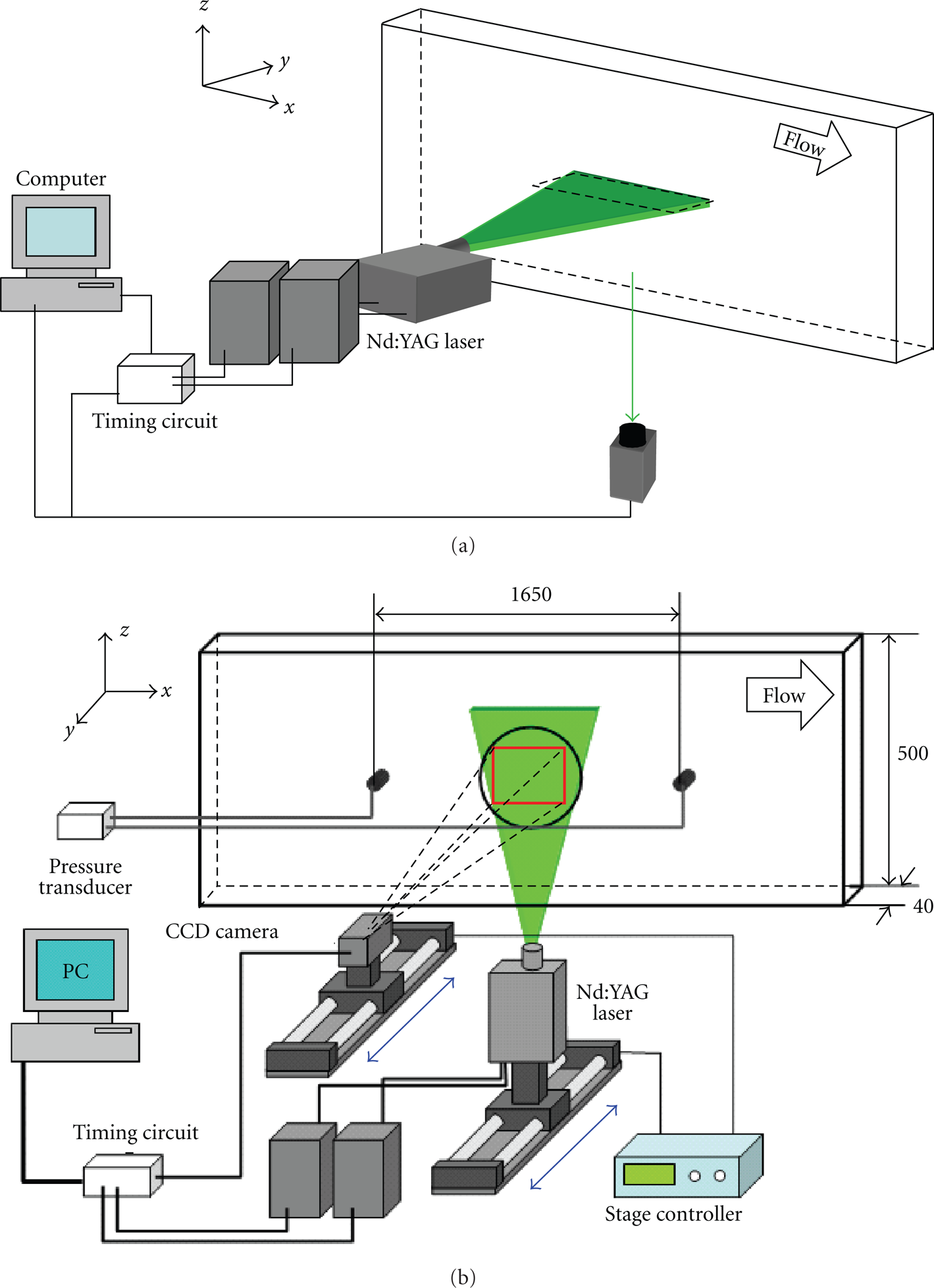
PIV system arrangement for measurements (a) in the x-y plane and (b) in the x-z plane.

The PIV system consisted of a double-pulse laser, laser sheet optics, CCD camera, synchronizer, and a computer with image-processing software (Dantec, Dynamics Studio version 2.30). The double-pulse laser (New Wave Research Co. Ltd., MiniLase-II/30 Hz) was a combination of a pair of Nd : YAG lasers, each having an output of 30 mJ/pulse and wavelength of 532 nm. The pulse interval was set to range from 300 μs to 500 μs considering the displacement of particles while measuring flow velocity. The laser sheet thickness and spread angle were set to 0.6 mm and 20°, respectively. The synchronization device communicated with the CCD camera and the computer, and generated pulses to control the double-pulse laser. The CCD camera had a resolution of 2048×2048 pixels and pixel pitch of 7.4×7.4 μm. The camera lens had a focal length of 60 mm and an aperture of 2.8. The flow was seeded with acrylic colloids to act as tracer particles. These particles were 0.1–1 μm in mean diameter. The particle concentration was adjusted so that more than 10 particles were observed on average in the interrogation area for each experiment. The interrogation area was 64×64 pixels with a cross-correlation with each interrogation area overlapping by 75%.

In this study, we measured the instantaneous velocity u-v in the x-y plane and u-w in the x-z plane by using PIV. For the measurements in the x-y plane, the measurement field was set to 70 mm (streamwise direction) × 40 mm (channel height). We obtained 125×65 vectors for each direction in the instantaneous velocity fields. Turbulence statistics were calculated from 500 velocity vector fields. On the other hand, for the measurements in the x-z plane, the instantaneous velocity was measured at 40 positions in the y direction, 0.5 mm to 20 mm from the wall at intervals of 0.5 mm, presuming the flow was symmetrical. The measurement field was set to 80 mm (streamwise direction) × 80 mm f(spanwise direction). There were 125×125 vectors in the x-z plane in each measurement field. Turbulent statistics were calculated from 100 velocity fields at each y position.

The Reynolds number was defined by the following equation based on the channel height and ranged from 10000 to 25000:

Re = \frac{U_{b} H}{v},

(1)

where H is the channel height and ν is the kinematic viscosity of water. Because we used a dilute surfactant solution in our experiment, the kinematic viscosity of the surfactant solutions was not so different from that of water [21].

2.2. Surfactant Solution

The surfactant used in this experiment was a cationic surfactant, cetyltrimethyl ammonium chloride (CTAC: C₁₆H₃₃N(CH₃)₃Cl), which had a molecular weight of 320.0 g/mol. Local tap water was used as a solvent because CTAC is hardly affected by the metallic ions of calcium and sodium which naturally exist in tap water. Sodium salicylate (NaSal), with a molecular weight of 160.1 g/mol, was added to this surfactant solution in the same weight concentration in order to provide counter ions. A diluted surfactant solution can produce drag-reduction due to counter ions being in a lower concentration than the critical micelle concentration (CMC). The concentration of the surfactant solution was 25 ppm or 40 ppm.

3. Results and Discussion

3.1. Drag-Reduction Rate

Table 1 shows the drag-reduction rate in each experimental condition. We performed PIV measurement in the x-y plane with different Reynolds numbers, but the Reynolds number was fixed at 20000 for the measurement in the x-z plane. In this paper, the experimental results for each condition are shown by the code name listed in this table.

Table 1:

Drag-reduction rate.

Code	Measurement	Fluid	Re	DR (%)

W-10	x-y	Water	10000	—
W-15		Water	15000	—
W-20		Water	20000	—
W-25		Water	25000	—

C25–10	x–y	CTAC 25 ppm	10000	33
C25–15		CTAC 25 ppm	15000	48
C25–20		CTAC 25 ppm	20000	59
C25–25		CTAC 25 ppm	25000	62

C40–10	x-y	CTAC 40 ppm	10000	32
C40–15		CTAC 40 ppm	15000	34
C40–20		CTAC 40 ppm	20000	52
C40–25		CTAC 40 ppm	25000	59

W-20-z	x-z	Water	20000	—
C25–20–z		CTAC 25 ppm	20000	59
C40–20–z		CTAC 40 ppm	20000	57

The drag-reduction rate is defined by the following equation:

DR = \frac{C_{f, w} - C_{f, s}}{C_{f, w}} \times 100 (%),

(2)

where C_f is the friction coefficient, and the subscripts w and s represent water and surfactant solution, respectively. The friction coefficient was calculated by

C_{f} = \frac{τ_{w}}{1 / 2 ρ U_{b}^{2}},

(3)

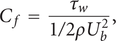
where τ_w is the wall shear stress obtained from the static pressure gradient of the channel, and ρ is the density of the water.

The drag-reduction rate increases with increasing Reynolds number, and a 62% maximum drag-reduction rate was obtained. Generally speaking, drag-reduction is related to the existence of a thread-like micelle network in the surfactant solution. Wunderlich and Brunn [22] reported that long thread-like micelles form under high shear rate in the surfactant solution and a shear induced state (SIS) occurs. These thread-like micelles are formed under suitable conditions of steady shear, surfactant concentration, and temperature. It is well known that there is a critical Reynolds number which has a maximum drag-reduction rate in surfactant drag-reducing flow as shown in Figure 3. Li et al. [18] categorized the relationship between Reynolds number and friction coefficient in the case of CTAC 25 ppm at 30°C into the following four regimes: (i) laminar, (ii) increase of drag-reduction rate, (iii) decrease of drag-reduction rate, and (iv) loss of drag-reduction rate as shown in Figure 3. In regime (ii), the drag-reduction rate increases with increasing Reynolds number because moderate shear assists the formation of the micellar network. However, in regime (iii), the micellar network cannot be formed because of the large shear stress. Therefore, the drag-reduction rate decreases in this regime. Moreover, they concluded that a critical Reynolds number with a maximum drag-reduction rate exists between regime (ii) and regime (iii). The value of the critical Reynolds number is affected by the surfactant concentrations and temperatures.

Figure 3:

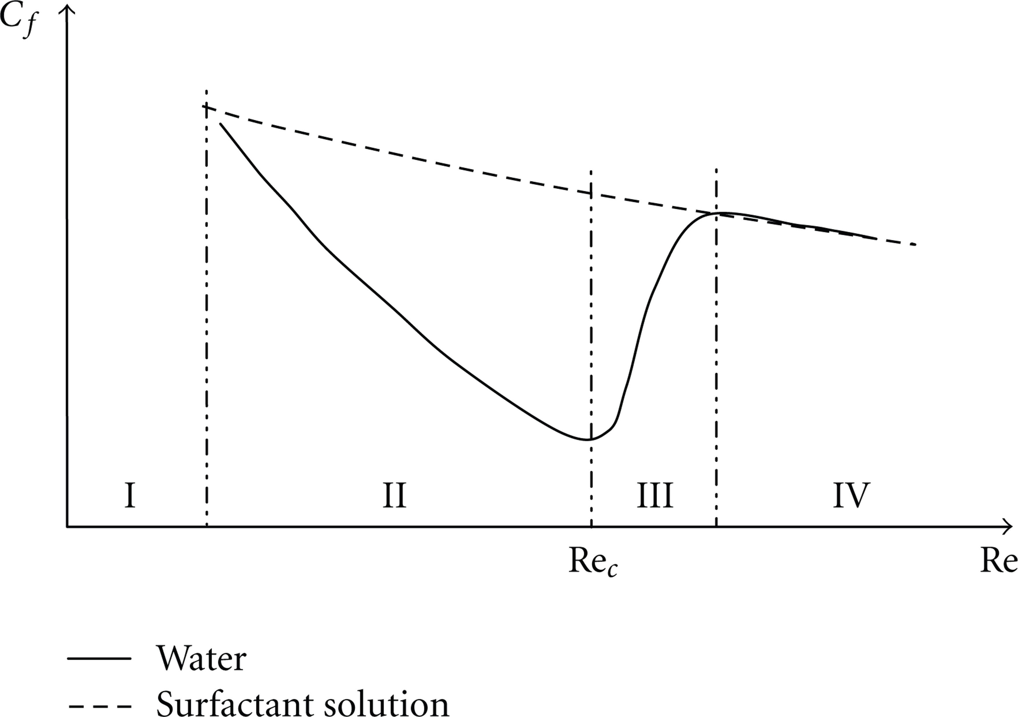
Schematic relationship between friction coefficient and Reynolds number.

Figure 4 shows the result of detailed measurement of the friction coefficient for each concentration of CTAC solution at 25°C. In this figure, the solid line represents the friction coefficient of the two-dimensional rectangular duct flow obtained by Dean [23]:

C_{f} = 0.073 {Re}^{- 1 / 4} .

(4)

Figure 4:

Reynolds number dependence on the friction coefficient.

The critical Reynolds number shifts to a large value with increasing surfactant concentrations. In our experiment, the critical Reynolds number does not agree with the results obtained by Li et al. [18], but the trend corresponds to their results. Because the critical Reynolds number is over 25000 in both concentrations, the drag-reduction rate increases with increasing Reynolds number in both concentrations, and this trend corresponds to the regime (ii).

3.2. Mean Streamwise Velocity

Figure 5 shows the mean streamwise velocity profiles in the water flow at Re=25000 and in CTAC solution for each Reynolds number. U⁺ is defined as the mean velocity $\overset{̅}{U}$ normalized by friction velocity u_τ and y⁺ is defined as position y normalized by ν/u_τ.

Figure 5:

Mean streamwise velocity profiles of the water flow and the drag-reducing flow.

The solid line in this figure represents the linear profile and log-law profile of streamwise velocity for Newtonian turbulent flow. The viscous sublayer is expressed by the following equation:

U^{+} = y^{+} .

(5)

In addition, the buffer layer and the logarithmic layer are expressed by

U^{+} = 2.4 \ln y^{+} + 5.5 .

(6)

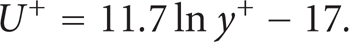
For comparison with our experiment, Virk's ultimate profile in the polymer drag-reducing flow, which was obtained by Virk et al. [24], is plotted using a dashed line in Figure 5. This line represents the following equation:

U^{+} = 11.7 \ln y^{+} - 17 .

(7)

In the water flow, the measured velocity profile is in good agreement with the log-law profile of the turbulent flow of Newtonian fluid. In the drag-reducing flow, the mean velocity profiles are upshifted in the log-law layer with a larger gradient compared with that in the water flow. Of particular significance is that the profile has the same gradient as Virk's ultimate profile at the high drag-reduction rate. According to Warholic et al. [25], if the drag-reduction rate is more than 35% (large drag-reduction), the velocity profile is displaced upward and the gradient increases with increasing drag-reduction rate. Therefore, our result with the homogeneous surfactant solution corresponds to the experimental results with the homogeneous polymer solution obtained by Warholic et al.

3.3. Turbulent Intensity

Figure 6 shows the effect of the Reynolds number on the distribution of the RMS of the streamwise velocity fluctuation u_rms normalized by the friction velocity u_τ for 25 ppm surfactant solution. The horizontal axis is normalized by half of the channel height δ. In the water flow, the streamwise velocity fluctuation monotonously decreases from the near-wall to the center of the channel. On the other hand, in the drag-reducing flow, the streamwise velocity fluctuation has a larger value than that of the water flow. Notably, an area appeared where the streamwise velocity fluctuation sharply decreased toward the center of the channel in the drag-reducing flow. For example, in the case of C25–10 (i.e., Re=10000 and CTAC 25 ppm), this area exists in the range of y/δ from 0.4 to 0.8. This indicates that two different layers coexist on the boundary of this area.

Figure 6:

Distribution of RMS of streamwise velocity fluctuation for the 25 ppm surfactant solution.

Figure 7 shows the same as Figure 6 obtained by the measurement in the x-z plane. Although the value of the velocity fluctuation is slightly different from the results by the measurements in the x-y plane, the trend corresponds to Figure 6. This Figure represents more clearly the structure of the two layers as mentioned in Figure 6.

Figure 7:

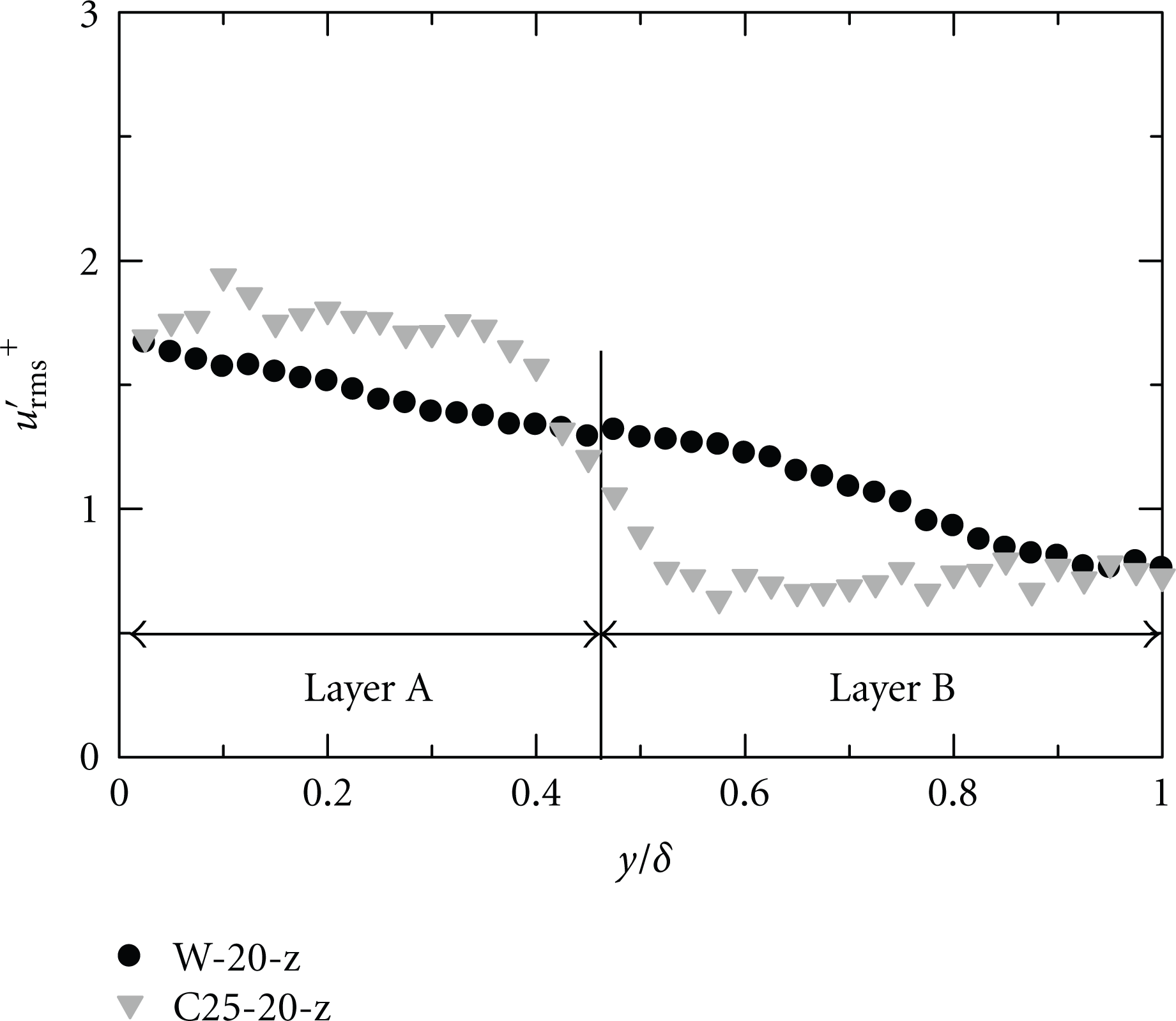
Same as Figure 6 for C25–20 obtained by the measurement in x-z plane.

In this paper, we define these two layers as “Layer A” and “Layer B” as shown in Figure 7. Moreover, h_A is defined as the thickness of Layer A. Comparing Layer A with Layer B, the value of the streamwise velocity fluctuation of Layer A is larger than that of Layer B. As shown in Figure 6, Layer A seems to expand to the center of the channel as the drag-reduction rate increases. A similar tendency was observed with a CTAC of 40 ppm. Therefore, the thickness of the two layers depends on the drag-reduction rate. A detailed discussion of this bilayer structure will be given in another section. In the case of turbulent boundary flow, a characteristic distribution of the streamwise velocity fluctuation was also observed in the drag-reducing flow [19, 20]. However, the detailed structure of these peaks has not been discussed.

The distribution of RMS of wall-normal velocity fluctuation v_rms normalized by the friction velocity for the 25 ppm surfactant solution is shown in Figure 8. In the drag-reducing flow, the wall normal velocity fluctuation is much smaller than that of the water flow throughout the channel height. In addition, the decrease level of the wall normal fluctuation is much higher than the increase level of the streamwise velocity fluctuation. This fact suggests that the turbulent energy transport between the different directional components is inhibited by the effect of additives. Therefore, the directional components become anisotropic in the drag-reducing flow.

Figure 8:

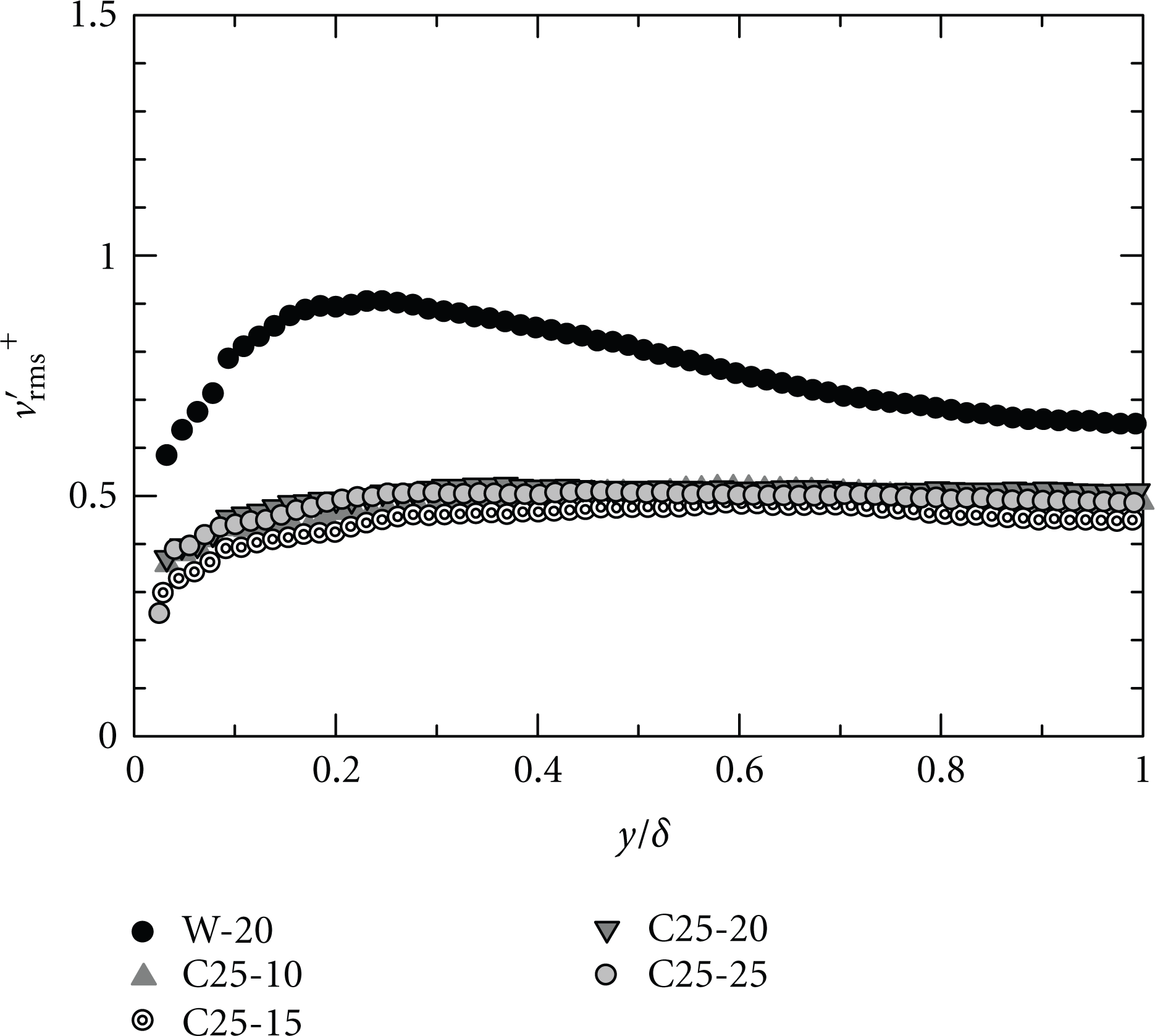
Distribution of RMS of wall-normal velocity fluctuation for 25 ppm surfactant solution.

Moreover, we observed a slight peak in the wall normal velocity fluctuation at y/δ=0.2 in the water flow. This peak almost disappeared and the wall normal velocity fluctuation slightly increased toward the center of the channel. This seemed to indicate that the buffer layer expands to the center of the channel in the drag-reducing flow. Yu and Kawaguchi [26] investigated the drag-reducing channel flow by DNS and reported that adding surfactant additives to the water flow altered the energy redistribution. Surfactant additives inhibit the input energy transfer from mean flow to turbulent production, and inhibit energy transfer from the streamwise velocity component to the wall-normal and spanwise velocity components because of the large extensional viscosity. A similar result seems to have been obtained in our experiment.

3.4. Reynolds Shear Stress

Figure 9 shows the distribution of the Reynolds shear stress of the water flow and the drag-reducing flow of the 25 ppm surfactant solution, normalized by the friction velocity. In the drag-reducing flow, Reynolds shear stress is almost zero throughout the channel. This indicates that the momentum transport mechanism of the drag-reducing flow is quite different from that of the Newtonian fluid flow. A similar tendency was also found for the 40 ppm surfactant solution.

Figure 9:

Distribution of Reynolds shear stress for the 25 ppm surfactant solution.

The viscoelastic effect of the surfactant solution also appears to increase the velocity fluctuation. Actually, in the drag-reducing channel flow with surfactant solution, the correlation between the streamwise velocity fluctuation and the wall-normal velocity fluctuation decreases, as does the Reynolds shear stress due to the effect of the surfactant solution. A similar result of an increase in fluctuation was reported in turbulent boundary layer experiments with a surfactant solution conducted by Tamano et al. [20]. In addition, an increase in the Reynolds number corresponded to an increase of the Weissenberg number defined by relaxation time and friction velocity. Tsukahara et al. [27] and Yu and Kawaguchi [28] carried out a DNS study of the drag-reducing flow using the Giesekus model for surfactant solutions and investigated the relation between the Weissenberg number and drag-reduction. According to their calculations, high drag-reduction can be achieved by suppressing the production of turbulence for a high Weissenberg number. Therefore, our experimental results match those of their DNS study.

3.5. Vorticity Intensity

We calculated turbulent statistics of vorticity fluctuation ω_y^′. ω_y is defined in the following equation:

ω_{y} = \frac{\partial w}{\partial x} - \frac{\partial u}{\partial z} .

(8)

In this study, the calculational procedure of ω_y is based on the circulating volume of the surrounding 8 velocity values as shown in Figure 10. Therefore, ω_y in the position (i,j) is expressed with the following equation:

{({\overset{̅}{ω}}_{y})}_{i, j} = \frac{1}{A} Γ_{i, j} = \frac{1}{A} \oint_{l (X, Z)} (U, W) \cdot d l,

(9)

where A represents the circulation pathway.

Figure 10:

Calculation route of vorticity in the position (i, j).

Figure 11 shows the effect of the surfactant concentration on the distribution of the vorticity fluctuation ω_{y
r
m
s}^* for Re=20000. ω_{y
r
m
s}^* is normalized by the following equation:

ω_{y r m s}^{*} = \frac{ω_{y r m s}^{'} \cdot (H / 2)}{U_{b}} .

(10)

Figure 11:

Effect of surfactant concentration on the distribution of the vorticity fluctuation at Re=20000.

This figure indicates that the vorticity fluctuation monotonously decreases from the near-wall to the center of the channel in the water flow. On the other hand, the vorticity fluctuation in the drag-reducing flow is much smaller than that in water flow throughout the channel height. This suggests that the turbulent vortex is suppressed in the drag-reducing flow, and drag-reduction occurs. Similar to the distribution of the streamwise velocity fluctuation, Layer A and Layer B can be observed in the same area. In addition, the value of the vorticity fluctuation of Layer A is larger than that of Layer B.

Figure 12 shows the instantaneous vorticity fluctuation map in the water flow obtained by the measurement in the x-z plane. In this figure, (a) and (b) show the structure in the near-wall region (y/δ=0.025) and at the center of the channel (y/δ=1.0), respectively. The contour is determined from the value of the vorticity fluctuation at each position, and a positive value indicates a clockwise rotation. In the case of the water flow, although the value of the vorticity fluctuation is different, the flow patterns are similar to each position. In addition, similar patterns were also observed at all other positions in the water flow.

Figure 12:

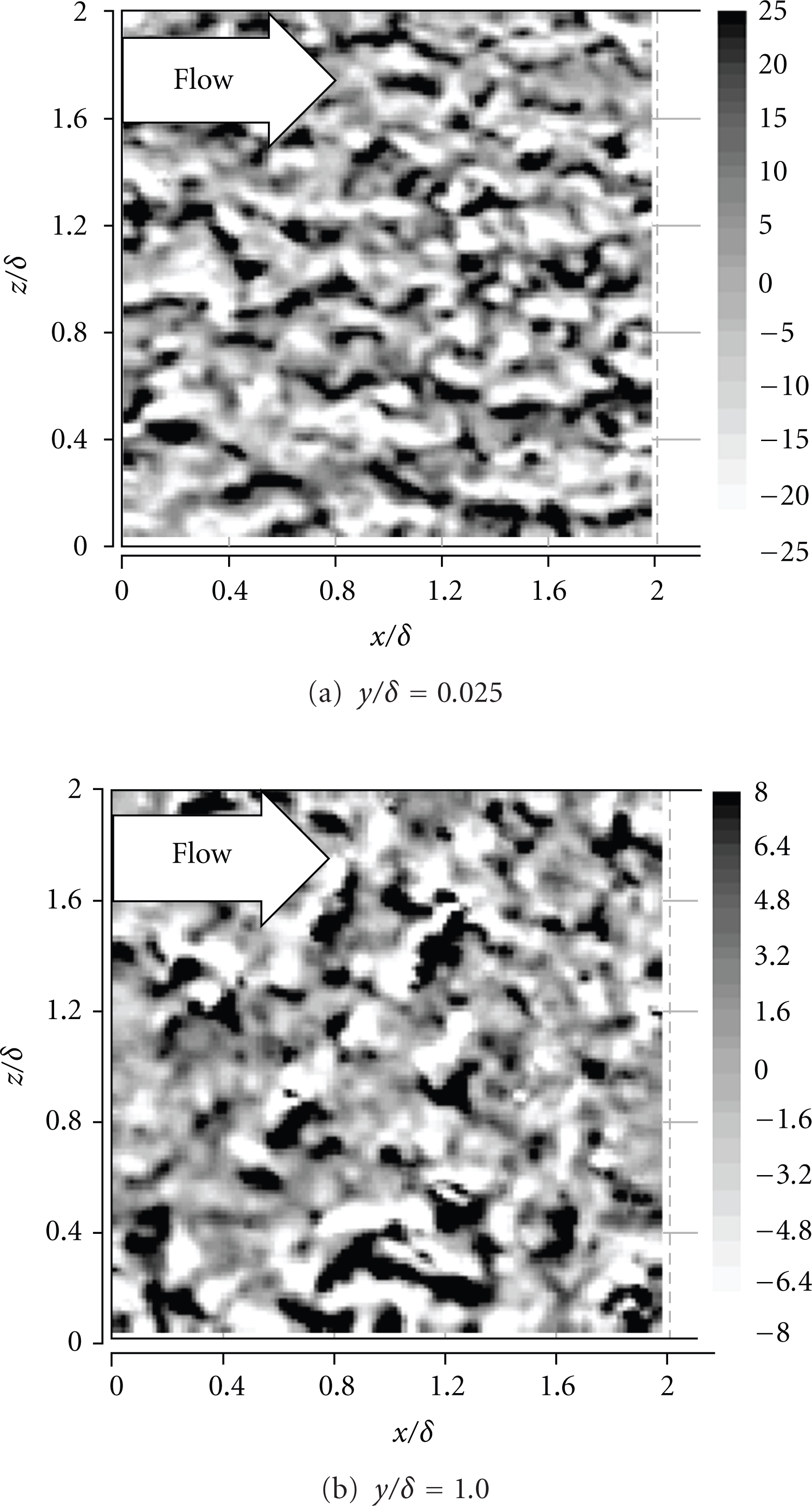
Instantaneous vorticity fluctuation map of the water flow at Re=20000; (a) y/δ=0.025 and (b) y/δ=1.0.

On the other hand, Figure 13 shows an instantaneous vorticity fluctuation map in the drag-reducing flow at the position (a) y/δ=0.025 (i.e., the near-wall region), (b) y/δ=0.4 (i.e., edge of Layer A), (c) y/δ=0.6 (i.e., edge of Layer B) and (d) y/δ=1.0 (i.e. center of the channel), respectively. In Layer A (see Figures 13(a) and 13(b)), the distribution of the vorticity fluctuation pattern shows a striped structure. In contrast, quite a different structure was observed in Layer B (see Figures 13(c) and 13(d)). It had a grained structure and this structure was similar to the pattern of the water flow but the spatial structure scale was much smaller (see Figure 12). In Layer A, the striped structure seemed to stretch along streamwise, and streaks with a variety of lengths were observed. The pattern was not very different from that for other Reynolds numbers or concentrations.

Figure 13:

Instantaneous vorticity fluctuation map of the drag-reducing flow for Re=20000; (a) y/δ=0.025, (b) y/δ=0.4, (c) y/δ=0.6, and (d) y/δ=1.0.

In our previous study [29], we measured the instantaneous velocity of the drag-reducing channel flow in the x-y plane by using a PIV system with a large measurement field. As a result, in the drag-reducing flow, there were large-scale fluid lumps in the near wall region. These structures extended toward the streamwise direction and were inclined at approximately 10 degrees to the channel wall. These characteristic structures were only observed in the case of high drag-reduction rate, and the tendency of these structures did not change with varying Reynolds number. The striped structure which stretches to the streamwise direction corresponds to this large-scale structure.

3.6. Discussion of the Bilayer Structure

Figure 14 shows the schematic interpretation of the relation between the thickness of two layers and the drag-reduction rate. When the drag-reduction rate increases, the thickness of Layer A spreads to the center of the channel. On the other hand, in the case of a low drag-reduction rate, Layer A is thin. This characteristic difference of structure seems to be attributed to SIS, which is characteristic of viscoelastic fluid. In Layer A, SIS occurs and contributes to the drag-reduction. In contrast, Layer B does not contribute to the drag-reduction and SIS does not occur because the instantaneous vorticity fluctuation map is similar to the water flow in this layer.

Figure 14:

Schematic interpretation of relation between thickness of two layers and the drag-reduction rate.

Yu and Kawaguchi [30] and Wu et al. [17] investigated drag-reducing channel flow using the Giesekus model by DNS. They applied a bilayer model, in which Newtonian and non-Newtonian fluids coexist. In their calculation, the interface between two layers sets to parallel to the wall and normal stress balance equation was satisfied. If the network structure (non-Newtonian fluids) exists in the near-wall region, the thickness of this layer spreads with increasing drag-reduction rate. Comparing the distribution of turbulent intensity between our experiment and their DNS results, they found that the distribution of the streamwise velocity fluctuation had the same or a larger value compared to the water one, but the distribution of the wall normal velocity distribution was smaller than the water one. Similar results were obtained in our experiment except for the area where the streamwise velocity fluctuation sharply decreased toward the center of the channel in the drag-reducing flow.

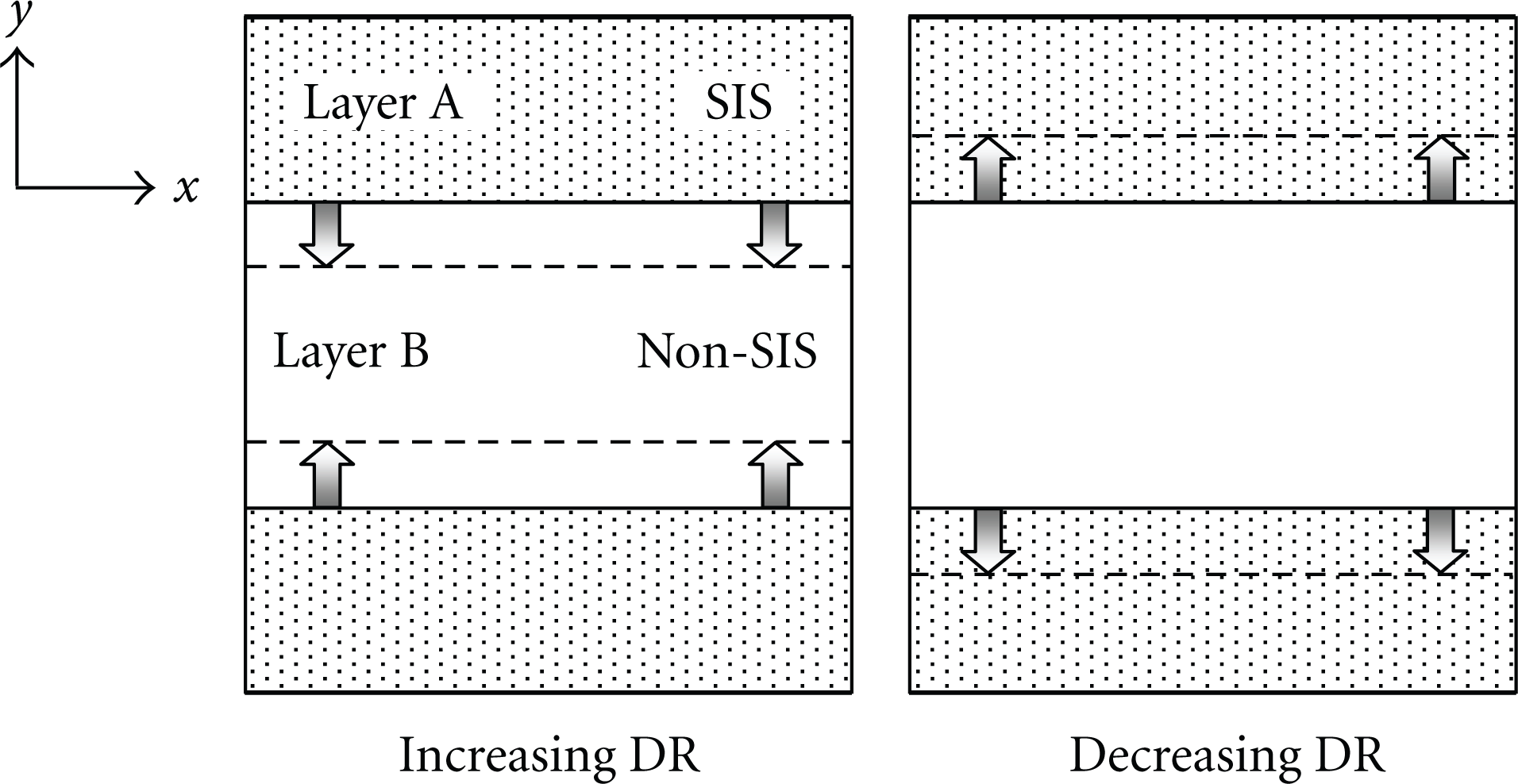
Figure 15 shows a schematic interpretation of the relation between the thickness of the two layers and the friction coefficient (i.e., drag-reduction rate). When the drag-reduction rate increased (i.e., a friction coefficient decreased) before the critical Reynolds number, the Non-Newtonian fluid (SIS) which contributed to drag-reduction existed in the near-wall region due to moderate shear stress, and the thickness of this layer spread to the center of the channel like (A) and (B) as shown in Figure 15, and in the region away from the wall (i.e., Newtonian fluid), shear stress was not enough for SIS to occur. Then, as the Reynolds number reached a critical point, the Non-Newtonian fluid spread all over the channel represented as (C) and the drag-reduction rate reached the maximum. Beyond the critical Reynolds number, drag-reduction rate decreased and non-Newtonian fluid existed in a region away from the wall, like (D) and (E). This was because the shear rate near the wall was so large it could not form a network structure in the near-wall region. Finally, as the Reynolds number increased more, drag-reduction vanished due to the high shear rate all over the channel and the non-Newtonian fluid disappeared as shown (F).

Figure 15:

Detailed discussion of the relation between the bilayer structure and drag-reduction.

In our experiment, because a large drag-reduction occurred, the flow structure seemed to be like (B) or (C). In addition, we observed that the flow pattern of Layer B was similar to the water flow. Although there is no conclusive evidence that Layer A has similar characteristics to the non-Newtonian fluids, the bilayer structure observed in our experiment corresponds to these DNS results. More detailed experiments will be performed to clarify the flow structures of the two layers in the drag-reducing surfactant flow in the future.

3.7. Summary of the Zonal Structure

Finally, we describe briefly the zonal structure of the drag-reducing channel flow observed in this study and previous studies [29]. As shown in Figure 7, there appeared an area where the streamwise velocity fluctuation sharply decreased toward the center of the channel in the drag-reducing flow. Therefore, two layers having different structures appear to coexist on the boundary of this area in the drag-reducing channel flow. The structure near the center of the channel (Layer B) has a grained pattern, which is similar to the pattern of the water flow. On the other hand, the structure in the near-wall region (Layer A) has a striped pattern which extends in the streamwise direction. The pattern is not so different at other Reynolds numbers or concentrations but the thickness of Layer A spreads to the channel center as the drag-reduction rate increases. According to our previous study [29], sweep and ejection are greatly suppressed and large-scale inclined fluid lumps appear alternately in Layer A. In contrast, these fluid lumps do not appear in the center of the channel (Layer B). For the same CTAC concentration, the scale and inclination angle of these large-scale structures did not depend on Reynolds number and rheological parameters.

4. Conclusions

Characteristic zonal structures of the drag-reducing channel flow with surfactant additives were investigated experimentally. We performed PIV measurement of the instantaneous velocity in the x-y plane and in the x-z plane with changing Reynolds number and the weight concentration of CTAC. The following conclusions on the drag-reducing flow were obtained.

The distribution of the wall normal velocity fluctuation in the drag-reducing flow was much smaller than that of the water flow and Reynolds shear stress in the drag-reducing flow was almost zero throughout the channel.

The streamwise velocity fluctuation monotonously decreased from the near-wall to the center of the channel in the water flow, but an area appeared where the streamwise velocity fluctuation sharply decreased toward the center of the channel in the drag-reducing channel flow. This indicated that two layers having different structures appeared to coexist on the boundary of this area. The distribution of the vorticity fluctuation also sharply decreased in the same area.

The layer in the near-wall region had a striped structure, and the layer in the center of the channel had a grained structure. This grained structure was similar to the flow structure of the water flow. The thickness of the layer in the near-wall region expanded toward the center of the channel as the drag-reduction rate increased. These characteristic differences seem to be attributed to the SIS and viscoelasticity of the fluid.

Footnotes

Acknowledgments

The authors would like to thank Mr. A. Saito of Mitsubishi Heavy Industries, Ltd., and Mr. D. Tsurumi of the Tokyo University of Science for their collaboration in this study.

References

Toms

B. A.

, “Some observations on the flow of linear polymer solutions through straight tubes at large Reynolds numbers,” in Proceedings of the 1st International Congress on Rheology, pp. 135–141, Amsterdam, The Netherlands, 1978.

Burger

E. D.

Munk

W. R.

, and Wahl

H. A.

, “Flow increase in the Trans Alaska Pipeline through use of a polymeric drag-reducing additive,” Journal of Petroleum Technology, vol. 34, no. 2, pp. 377–386, 1982.

Cox

L. R.

Dunlop

E. H.

, and North

A. M.

, “Role of molecular aggregates in liquid drag reduction by polymers,” Nature, vol. 249, no. 5454, pp. 243–245, 1974.

Kadoma

I. A.

Ylitalo

, and Van Egmond

J. W.

, “Structural transitions in wormlike micelles,” Rheologica Acta, vol. 36, no. 1, pp. 1–12, 1997.

Scriven

L. E.

Davis

H. T.

Talmon

, and Zakin

J. L.

, “Effect of chemical structure on viscoelasticity and extensional viscosity of drag-reducing cationic surfactant solutions,” Langmuir, vol. 14, no. 1, pp. 8–16, 1998.

and Matthys

E. F.

, “Rheological and rheo-optical characterization of shear-induced structure formation in a nonionic drag-reducing surfactant solution,” Journal of Rheology, vol. 41, no. 1, pp. 151–166, 1997.

and Matthys

E. F.

, “Characterization of micellar structure dynamics for a drag-reducing surfactant solution under shear: normal stress studies and flow geometry effects,” Rheologica Acta, vol. 34, no. 5, pp. 450–460, 1995.

Gasljevic

and Matthys

E. F.

, “Field test of a drag-reducing surfactant additive in a hydronic cooling system,” in Proceedings of the ASME Fluids Engineering Division Summer Meeting, vol. 237, pp. 249–260, 1996.

Takeuchi

, “Actual proof test of energy conservation in central heating/cooling system adapting surfactant drag reduction,” in Proceedings of the 8th International Conference on Sustainable Energy Technologies, Aachen, Germany, 2009.

10.

Warholic

M. D.

Heist

D. K.

Katcher

, and Hanratty

T. J.

, “A study with particle-image velocimetry of the influence of drag-reducing polymers on the structure of turbulence,” Experiments in Fluids, vol. 31, no. 5, pp. 474–483, 2001.

11.

Dimitropoulos

C. D.

Sureshkumar

Beris

A. N.

, and Handler

R. A.

, “Budgets of Reynolds stress, kinetic energy and streamwise enstrophy in viscoelastic turbulent channel flow,” Physics of Fluids, vol. 13, no. 4, pp. 1016–1027, 2001.

12.

Somandepalli

V. S. R.

Hou

X. Y.

, and Mungal

M. G.

, “Turbulent schmidt number measurements in a polymer drag-reduced turbulent boundary layer,” in Proceedings of the 6th International Symposium on Turbulence and Shear Flow Phenomena, Seoul, Korea, 2009.

13.

Wang

Wei

J. J.

F. C.

, and Kawaguchi

, “Direct numerical simulation on drag-reducing flow by poly-mer additives using a spring-dumbbell model,” Progress in Computational Fluid Dynamics, vol. 9, no. 3–5, pp. 217–224, 2009.

14.

White

C. M.

and Mungal

M. G.

, “Mechanics and prediction of turbulent drag reduction with polymer additives,” Annual Review of Fluid Mechanics, vol. 40, pp. 235–256, 2008.

15.

Kawaguchi

, “Turbulent transport mechanism in a drag-reducing flow with surfactant additive investigated by two component LDV,” in Proceedings of the 8th International Symposium on Applications of Laser Techniques to Fluid Mechanics, pp. 4. 1–4.7, Lisbon, Portugal, 1996.

16.

, and Kawaguchi

, “Numerical and experimental investigation of turbulent characteristics in a drag-reducing flow with surfactant additives,” International Journal of Heat and Fluid Flow, vol. 25, no. 6, pp. 961–974, 2004.

17.

, “DNS study on heat transfer reduction of drag-reducing channel flow induced by surfactant additives with a bilayer mode,” in Proceedings of the 2nd Asian Symposium on Computational Heat Transfer and Fluid Flow, pp. 175–181, Jeju, Korea, 2009.

18.

F.-C.

Kawaguchi

Segawa

, and Hishida

, “Reynolds-number dependence of turbulence structures in a drag-reducing surfactant solution channel flow investigated by particle image velocimetry,” Physics of Fluids, vol. 17, no. 7, pp. 1–13, 2005.

19.

Itoh

and Tamano

, “Drag reduction of turbulent flows of surfactant solutions,” in Proceedings of the 7th JSME-KSME Thermal and Fluids Engineering Conference, Sapporo, Japan, 2008.

20.

Tamano

Itoh

Inoue

Kato

, and Yokota

, “Turbulence statistics and structures of drag-reducing turbulent boundary layer in homogeneous aqueous surfactant solutions,” Physics of Fluids, vol. 21, no. 4, Article ID 045101, 2009.

21.

Kawaguchi

Wei

, and Feng

, “Rheological characterization of drag-reducing cationic surfactant solution -shear and elongational viscosities of dilute solutions,” in Proceedings of the 4th ASME/JSME Joint Fluids Engineering Conference, pp. 721–728, Honolulu, Hawaii, USA, July 2003.

22.

Wunderlich

A. M.

and Brunn

P. O.

, “The complex rheological behavior of an aqueous cationic surfactant solution investigated in a Couette-type viscometer,” Colloid & Polymer Science, vol. 267, no. 7, pp. 627–636, 1989.

23.

Dean

R. B.

, “Reynolds number dependence of skin friction and other bulk flow variables in two-dimensional rectangular duct flow,” Journal of Fluids Engineering, vol. 100, no. 2, pp. 215–223, 1978.

24.

Virk

, “The ultimate asymptote and mean flow structure in Toms phenomenon,” Journal of Applied Mechanics, vol. 37, no. 2, pp. 488–493, 1970.

25.

Warholic

M. D.

Massah

, and Hanratty

T. J.

, “Influence of drag-reducing polymers on turbulence: effects of Reynolds number, concentration and mixing,” Experiments in Fluids, vol. 27, no. 5, pp. 461–472, 1999.

26.

and Kawaguchi

, “Direct numerical simulation of viscoelastic drag-reducing flow: a faithful finite difference method,” Journal of Non-Newtonian Fluid Mechanics, vol. 116, no. 2–3, pp. 431–466, 2004.

27.

Tsukahara

, “DNS study on viscoelastic effect in drag-reduced turbulent channel flow,” Journal of Turbulence, vol. 12, pp. 1–25, 2010.

28.

and Kawaguchi

, “Effect of Weissenberg number on the flow structure: DNS study of drag-reducing flow with surfactant additives,” International Journal of Heat and Fluid Flow, vol. 24, no. 4, pp. 491–499, 2003.

29.

Motozawa

Watanabe

, and Kawaguchi

, “PIV measurements of large-scale structures in a drag-reducing channel flow with surfactant additives,” Nihon Reoroji Gakkaishi, vol. 39, no. 3, pp. 99–104, 2011.

30.

and Kawaguchi

, “DNS of drag-reducing turbulent channel flow with coexisting Newtonian and non-Newtonian fluid,” Journal of Fluids Engineering, vol. 127, no. 5, pp. 929–935, 2005.

Experimental Investigation on Zonal Structure in Drag-Reducing Channel Flow with Surfactant Additives

Abstract

1. Introduction

2. Experiment

2.1. Experimental Facility and PIV Procedure

2.2. Surfactant Solution

3. Results and Discussion

3.1. Drag-Reduction Rate

3.2. Mean Streamwise Velocity

3.3. Turbulent Intensity

3.4. Reynolds Shear Stress

3.5. Vorticity Intensity

3.6. Discussion of the Bilayer Structure

3.7. Summary of the Zonal Structure

4. Conclusions

Footnotes

Acknowledgments

References