Ranging Energy Optimization for a TDOA-Based Distributed Robust Sensor Positioning System

Abstract

The author proposes a distributed localization scheme for an asynchronous wireless sensor network (WSN) consisting of at least two beacons as well as some anchors, each collaborating with the beacons to help the sensors within the corresponding service area for self-localization. Most interestingly, each sensor does not need to emit either ranging or communication signals to neighbor sensors in the proposed scheme. Instead, each sensor only needs to estimate the time-of-arrivals (TOAs) of incoming ranging signals from the beacons and the anchors, and then the time-difference-of-arrival (TDOA) between the signal propagating from each beacon to the sensor and the one from that beacon to the sensor via an associated anchor is produced and converted to a range difference measurement at the sensor for self-localization. Assuming the location estimator adopted achieves the associated Cramér-Rao bounds (CRB), the localization performance at each sensor is derived and analyzed. When the system features robust sensor positioning (RSP) in that a prescribed accuracy requirement is fulfilled in all service areas of the anchors, the author considers ranging energy optimization problems related to the beacons and the anchors, and presents practical algorithms to solve them. The effectiveness of those algorithms is illustrated by numerical experiments.

1. Introduction

Wireless sensor networks (WSNs) envision a variety of attractive applications, such as target tracking, intrusion detection, and environmental monitoring, just to name a few [1]. The WSNs usually consist of asynchronous small nodes which are battery-powered and inexpensive, but possess limited capabilities of sensing, computation, and communication. Depending on the application of WSNs, either each node or a control center must be aware of the node's position with sufficiently high accuracy, since sensed data are often useless if we do not know where they are sensed. However, most of the WSNs are deployed by spreading the nodes randomly over a prescribed service area. Therefore, node localization in WSNs has been attracting intensive research interest lately.

We consider in this paper the localization of asynchronous nodes in WSNs. In particular, the localization accuracy for each node satisfies a prescribed requirement to achieve reliable location awareness. Perhaps the most well-known requirement is the one defined by the Federal Communication Commission (FCC) [2]. More specifically, it requires the location-estimation error to have a length smaller than $R_{\text{e}}$ with a probability higher than $P_{\text{e}}$ , where both $R_{\text{e}}$ and $P_{\text{e}}$ have prescribed values. We adopt this requirement for the WSN localization systems considered in this paper.

Equipping each node with a global positioning system (GPS) is a simple but inappropriate solution for the cost-effective or indoor WSNs. Instead, a few reference nodes with known positions, referred to as anchors hereafter, are encompassed in most of the WSNs to help in locating the position-unaware nodes, referred to as sensors hereafter. In particular, the anchors know their positions because they are manually installed or equipped with a GPS. During the localization process, position-related intersensor measurements as well as those between the sensors and the anchors are first obtained, then they are used in combination with the anchors' positions to estimate the sensors' positions. Typical measurements for localization purposes include connectivity, received-signal-strength (RSS), angle-of-arrival (AOA), time-of-arrival (TOA), and time-difference-of-arrival (TDOA). Note that AOA measurements are usually considered as inappropriate for WSNs since antenna arrays are needed but not practically affordable by the small sensors. The past few years have witnessed significant efforts in developing sensor localization algorithms based on the connectivity [3–6] or RSS measurements [7–10], since these measurements can be easily obtained even with low-cost radio hardware. However, they are only suitable for coarse sensor localization since in practice the connectivity and RSS measurements are subject to large variability due to unpredictable hardware imperfection as well as random propagation fading [8].

Plenty of localization algorithms based on range or range difference (RD) measurements, which are usually converted from TOA/TDOA measurements, have been proposed. In conventional localization algorithms, either the range measurements [11–14] or the RD measurements [15–20] between a sensor and the anchors are used at the sensor or the control center for estimating this sensor's position, depending on the specific application. Lately, a variety of collaborative algorithms, which make use of the extra intersensor measurements to improve performance, have been developed. Interestingly, all these collaborative algorithms are based on range measurements, and can be classified into two categories, namely, centralized collaborative algorithms (CCAs) and distributed collaborative algorithms (DCAs).

The CCAs need to collect all range measurements at a central processor for estimating all sensors' positions, and they are based on one of three techniques: maximum-likelihood (ML) estimation, convex optimization (CO), and multidimensional scaling (MDS). Though the ML-based CCAs are asymptotically efficient, they are usually implemented iteratively, and the performance is very sensitive to the initialization [21, 22]. The CO-based CCAs relax the original localization problems into semidefinite programming (SDP) problems [23–25] or second-order cone programming (SOCP) problems [26]. The classical MDS method can be applied to the localization of fully connected WSNs where all internode range measurements are available [27, 28]. For partially connected WSNs, the classical MDS method can be applied after reconstructing the missing internode distances by shortest-path distance measurements [29] or the singular value decomposition [30]. An alternative way is to compute local relative coordinates for fully connected node subsets, and then patch them together to produce global position estimates for the sensors with the help of the anchors' positions [31]. Recently, it was shown that MDS-related subspace approaches [32] and weighted MDS methods [33] yield better performance than the classical MDS method. The CCAs usually feature good performance with only a few internode communications for relaying the range measurements to the central processor.

The DCAs require every sensor to estimate its own position iteratively through a number of information exchanges with its neighbor nodes. Compared with the CCAs, the DCAs feature good scalability which suits large-scale WSNs. The DCAs can be grouped into generalized-multilateration (GM) DCAs and successive-refinement (SR) DCAs. As for the GM DCAs, each sensor estimates the distances to multiple anchors using either direct measurements if they exist, or shortest-path distance measurements to those anchors [34–36]. After that, each sensor estimates its own position by the classical multilateration techniques. As for the SR DCAs, each sensor iteratively updates its position estimate as a function of the range measurements to its neighbor nodes and the position estimates of those neighbor nodes. Specifically, the SR DCAs are based on one of four principles. The first is the maximum-a-posterior (MAP) based algorithms which represent the WSN as a factor graph, and employ belief-propagation-based methods to compute a MAP position estimate at each sensor [37, 38]. The second is the local multilateration-based algorithms in which each sensor localizes itself using multilateration with respect to its neighbor nodes [39–42]. The third is the global-optimization-based algorithms which require each sensor to update its position estimate iteratively, so that a global objective metric keeps descending until convergence [43, 44]. The fourth is the distributed-consensus-based algorithms in which each sensor's position estimate is iteratively updated as a linear weighted sum of its neighbor nodes' position estimates [45]. Compared with the GM DCAs, the SR DCAs usually yield better performance but require a greater number of internode communications until convergence. Note that the key issue for these DCAs is that a big number of iterations is usually required, which reduces the lifetime of the sensors since a considerable amount of sensors' energy has to be consumed for internode communications.

To use the above-mentioned schemes in asynchronous WSNs, every sensor is required to emit ranging and communication signals for generating range/RD measurements and exchanging information with neighbor sensors, respectively. On the one hand, the ranging energy of the nodes should be sufficiently high to produce the sufficiently accurate range/RD measurements. On the other hand, the ranging energy should be reduced to prolong system lifetime, especially for the sensors and the anchors powered by batteries. This raises an interesting question: how much ranging energy has to be allocated at least to the sensors and the anchors, so that the prescribed accuracy requirement is satisfied? It is very important to address this problem for every proposed scheme to be used in practice, but only the one for the two-way TOA-ranging-based scheme has been reported so far [46–48].

In this paper, we consider an asynchronous distributed WSN localization system, which consists of at least two position-known beacons as well as multiple anchors, each collaborating with the beacons to help the sensors within the corresponding service area for self-localization. The beacons are located at easily accessible positions so that they can use reliable power supplies, whereas the anchors are randomly deployed with sensors but equipped with higher capacity batteries than sensors. Specifically, our contributions lie in the following aspects.

• (i)

A novel localization scheme is proposed for the considered system. The advantage of this scheme over the above mentioned schemes is that, each sensor does not need to emit either ranging or communication signals for producing range/RD measurements or exchanging information with neighbor sensors, respectively. It only needs to estimate the TOAs of incoming ranging signals from the beacons and the corresponding anchor, and then the TDOA between the signal propagating from each beacon to the sensor and the one from that beacon to the sensor via the corresponding anchor is produced and converted to a RD measurement at the sensor for the self-localization. Under the assumption that the location estimator adopted achieves the associated Cramér-Rao bounds (CRBs), the localization performance at each sensor is derived and analyzed. Note that the CRB has been widely used to analyze the performance of WSN localization schemes [14, 22, 49–51].

(ii)

Ranging energy optimization problems related to the beacons and the anchors are considered, when the system features robust sensor positioning (RSP) in that a prescribed accuracy requirement is fulfilled in all service areas of the anchors. Practical algorithms are presented to solve them, and the effectiveness of those algorithms is illustrated by numerical experiments. Though we assume an optimistic scenario where the associated CRBs are achieved, the optimization results set lower bounds on the ranging energy required in realistic scenarios, and give a sense of how much ranging energy has to be allocated at least.

The rest of this paper is organized as follows. In the next section, we will describe the considered system. In Section 3, we will elaborate on the localization procedure and make a performance study. After that, we will propose ranging energy optimization problems, as well as practical algorithms to solve them in Section 4. In Section 5, numerical experiments will be presented. Finally, we wrap up this paper with some conclusions.

2. System Descriptions

We consider a 2-dimensional sensor positioning system with M beacons, where beacon m is located at a known coordinate ${\mathbf{p}}_m=[x_{\text{b},m},y_{\text{b},m}{]}^T$   ( $m=1,\dots ,M$ ). Note that M should be no smaller than 2, as will be explained in Section 3.1. The beacons are located at easily accessible positions so that they can use reliable power supplies such as power lines or high-capacity batteries regularly recharged without obstructing the functionality of the WSN. In addition, there exist N anchors, which are randomly deployed with sensors but have enhanced functionality, in that they are equipped with GPSs and higher capacity batteries than sensors. Note that these anchors may serve as local heads for constructing a clustered structure for the WSN [52]. Specifically, anchor n, located at a known coordinate ${\mathbf{q}}_n=[x_{\text{a},n},y_{\text{a},n}{]}^T$   ( $n=1,\dots ,N$ ), is responsible for collaborating with the beacons so that the sensors lying within a prescribed service area $S_n$ can locate themselves.

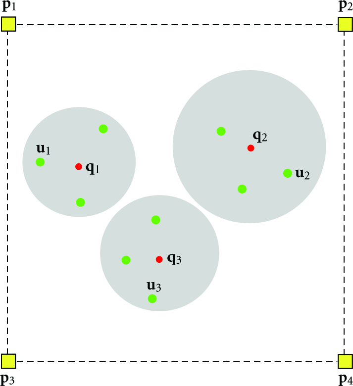
To distinguish the beacons and the anchors more clearly, let us consider a WSN where the proposed scheme can be carried out as shown in Figure 1. This WSN is deployed in a field for monitoring certain environmental parameters such as temperature. The beacons are manually installed at the corners of the field, so that their positions are perfectly known and they can use high-capacity batteries regularly recharged without hindering the WSN to carry out its tasks. The anchors are randomly deployed along with the sensors, but they are equipped with GPSs and batteries with higher capacity than the sensors, so that their positions are known and they can collaborate with the beacons to help the sensors within the corresponding service areas for self-localization.

Figure 1

An example WSN deployed in a 2-dimensional field for monitoring certain environmental parameters. The gray area surrounding each anchor represents the associated service area, and the green circles represent the sensors.

There is no infrastructure for coordinating beacons and anchors to emit ranging signals simultaneously. In addition, the clocks of beacons, sensors, and anchors are all asynchronous but run at the same pace, and the offset between any two of these clocks is unknown. This means that the one-way TOA (resp., TDOA) based scheme, which requires anchors and beacons to transmit ranging signals while each sensor to estimate their TOAs and produce range [11–13] (resp., RD [15–20]) measurements, is not applicable. To address this issue, the two-way TOA based scheme, which requires each sensor to estimate the round-trip TOA from it to every beacon or anchor and then produce the range measurements, can be adopted [47, 53]. However, this requires the sensor to emit a ranging signal, which is avoided by the proposed localization scheme to save the sensor's energy as will be shown in Section 3.1.

Each sensor within $S_n$ establishes a link with anchor n through certain protocol, for example, the one proposed in [52]. Before the localization procedure is carried out, all beacons' coordinates are broadcasted to all sensors and anchors, and anchor n's coordinate is broadcasted to all sensors in $S_n$ through some data packets. Let's say one of the sensors to be located within $S_n$ has an unknown coordinate ${\mathbf{u}}_n=[x_{\text{s},n},y_{\text{s},n}{]}^T$ . For notation simplicity, we refer to this sensor as sensor n hereafter. In this paper, we consider the scenario where a line-of-sight-propagation link exists between any two of sensor n, anchor n, and each beacon. This is the focus of many works on distributed WSN localization recently reported in the literature, for example, [41, 45, 47]. It is very interesting to investigate the scenario where some links' quality is degraded by nonline of sight propagation, which is part of our future work. To simplify system design, the sensor lying in the intersection of multiple service areas chooses only the anchor corresponding to the strongest link to connect with, then it produces measurements aided by that anchor for self-localization, as will be shown in Section 3.1. In fact, it can first establish links with all anchors serving all service areas where it lies, and then produces measurements with the help of all those anchors for self-localization. In this case, this sensor's localization performance is improved since more measurements carrying position-related information are used. This is a very interesting topic, which will be investigated in our future work.

Both the beacons and the anchors are capable of emitting ranging signals, and both the sensors and the anchors can estimate the TOAs of incoming ranging signals. The ranging signals used by the beacons are all the same and equal to $s_{\text{b}}(t)$ with energy $E_{\text{b}}$ , and the one used by anchor n is denoted by $s_{\text{a},n}(t)$ with energy ${ϵ}_n$ . In practice, these signals may be the preamble parts of communication signals emitted. $E_{\text{b}}$ and ${ϵ}_n$ are respectively above the threshold values $E_{\text{b}}^{\text{L}}$ and ${ϵ}_n^{\text{L}}$ that can be computed during the system design phase, so that the nodes in all service areas receive the beacons' ranging signals reliably, and each sensor in $S_n$ receives $s_{\text{a},n}(t)$ reliably. In addition, $E_{\text{b}}$ and ${ϵ}_n$ are respectively below $E_{\text{b}}^{\text{U}}$ and ${ϵ}_n^{\text{U}}$ determined by the hardware used or the spectral mask imposed to guarantee the coexistence of the considered sensor system with nearby radio systems.

We assume the robust sensor positioning (RSP) is achieved for the considered system, in the sense that a prescribed location accuracy requirement is fulfilled in the service areas of all anchors. Specifically, this requirement is that for all $n\in \{1,\dots ,N\}$ , for all ${\mathbf{u}}_n\in S_n$ , $\parallel {\widehat{\mathbf{u}}}_n-{\mathbf{u}}_n{\parallel }_2$ should be smaller than $R_{\text{e}}$ with probability higher than $P_{\text{e}}$ , where ${\widehat{\mathbf{u}}}_n$ denotes an estimate of ${\mathbf{u}}_n$ produced at sensor n, and the values of $R_{\text{e}}$ and $P_{\text{e}}$ are prescribed. To achieve the RSP with a reduced implementation complexity, $\{{ϵ}_n{\}}_{n=1}^N$ and $E_{\text{b}}$ are determined during the system design phase by solving the related ranging energy optimization problems proposed in Section 4.

As will be shown in Section 3.1, each beacon emits one ranging signal in every localization process, which means that a fair energy consumption strategy is assumed for beacons, since the ranging signals for different beacons are assumed to have the same energy. This assumption is reasonable for practical WSNs such as the example one described above, since it means all beacons can consume their energy at the same speed, so that their batteries can be recharged at the same time. Furthermore, it simplifies the localization-performance analysis, as well as solving the optimization problems in the following sections. It is interesting to consider the case when the beacons can use different ranging energy, which is part of our future work. On the other hand, we assume anchors can consume different amounts of ranging energy, because it is desirable to let each anchor use the corresponding smallest amount of ranging energy for the RSP, which might not be the same as for other anchors, since that energy depends on the location of the anchor and the size of the corresponding service area as will be shown in Section 4.2.

3. Localization Scheme and Performance Analysis

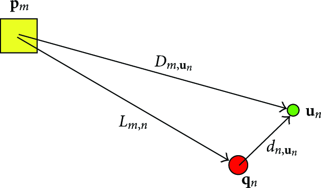
Before presenting the localization scheme and performance analysis, we define the following notations. $\parallel \mathbf{x}{\parallel }_2$ represents the Euclidean norm of a vector $\mathbf{x}$ . We denote the distance between beacon m and sensor n by $D_{m,{\mathbf{u}}_n}=\parallel {\mathbf{p}}_m-{\mathbf{u}}_n{\parallel }_2$ , the distance between anchor n and sensor n by $d_{n,{\mathbf{u}}_n}=\parallel {\mathbf{q}}_n-{\mathbf{u}}_n{\parallel }_2$ , and the distance between beacon m and anchor n by $L_{m,n}=\parallel {\mathbf{p}}_m-{\mathbf{q}}_n{\parallel }_2$ .

3.1. Localization Scheme

The localization scheme starts with the beacons broadcasting their ranging signals one after another. Let us say beacon m broadcasts $s_{\text{b}}(t)$ of energy $E_{\text{b}}$ . At sensor n, the TOA of this signal is denoted by $t_{{\mathbf{p}}_m\to {\mathbf{u}}_n}$ , but estimated by sensor n as ${\widehat{t}}_{{\mathbf{p}}_m\to {\mathbf{u}}_n}=t_{{\mathbf{p}}_m\to {\mathbf{u}}_n}+e_{{\mathbf{p}}_m\to {\mathbf{u}}_n}$ . At anchor n, the TOA of this signal is denoted by $t_{{\mathbf{p}}_m\to {\mathbf{q}}_n}$ , but estimated by anchor n as ${\widehat{t}}_{{\mathbf{p}}_m\to {\mathbf{q}}_n}=t_{{\mathbf{p}}_m\to {\mathbf{q}}_n}+e_{{\mathbf{p}}_m\to {\mathbf{q}}_n}$ . Here, $e_{{\mathbf{p}}_m\to {\mathbf{u}}_n}$ and $e_{{\mathbf{p}}_m\to {\mathbf{q}}_n}$ denote the TOA estimation error due to the presence of additive noise at sensor n and anchor n, respectively.

After estimating the TOAs of all the beacons' ranging signals, anchor n emits $s_{\text{a},n}(t)$ of energy ${ϵ}_n$ at time $t_{{\mathbf{q}}_n}$ to sensor n. We assume each anchor can measure $t_{{\mathbf{q}}_n}$ precisely with its internal clock, as in the works on WSN localization recently reported in the literature, for example, [47, 53]. At sensor n, the TOA of this signal is denoted by $t_{{\mathbf{q}}_n\to {\mathbf{u}}_n}$ , but estimated by sensor n as ${\widehat{t}}_{{\mathbf{q}}_n\to {\mathbf{u}}_n}=t_{{\mathbf{q}}_n\to {\mathbf{u}}_n}+e_{{\mathbf{q}}_n\to {\mathbf{u}}_n}$ , where $e_{{\mathbf{q}}_n\to {\mathbf{u}}_n}$ denotes the TOA estimation error at sensor n due to the presence of additive noise.

Note that $\{t_{{\mathbf{q}}_n\to {\mathbf{u}}_n},{\widehat{t}}_{{\mathbf{q}}_n\to {\mathbf{u}}_n}\}$ and $\{t_{{\mathbf{p}}_m\to {\mathbf{u}}_n},{\widehat{t}}_{{\mathbf{p}}_m\to {\mathbf{u}}_n}{\}}_{m=1}^M$ are according to the internal clock of sensor n, while $t_{{\mathbf{q}}_n}$ and $\{t_{{\mathbf{p}}_m\to {\mathbf{q}}_n},{\widehat{t}}_{{\mathbf{p}}_m\to {\mathbf{q}}_n}{\}}_{m=1}^M$ are according to the internal clock of anchor n. We can see that $t_{{\mathbf{q}}_n\to {\mathbf{u}}_n}-t_{{\mathbf{p}}_m\to {\mathbf{u}}_n}$ equals the time spent by the signals propagating along the path from beacon m to sensor n via anchor n, minus that by the signal from beacon m to sensor n directly. This is because $t_{{\mathbf{q}}_n\to {\mathbf{u}}_n}$ and $t_{{\mathbf{p}}_m\to {\mathbf{u}}_n}$ representing the TOAs of these two simultaneously emitted signals, respectively, are the points in the timeline corresponding to sensor n's clock. As illustrated in Figure 2, this difference is equal to $(L_{m,n}+d_{n,{\mathbf{u}}_n})/c+(t_{{\mathbf{q}}_n}-t_{{\mathbf{p}}_m\to {\mathbf{q}}_n})-(D_{m,{\mathbf{u}}_n}/c)$ , taking into account the processing delay $t_{{\mathbf{q}}_n}-t_{{\mathbf{p}}_m\to {\mathbf{q}}_n}$ at anchor n. This means that $c(t_{{\mathbf{q}}_n\to {\mathbf{u}}_n}-t_{{\mathbf{p}}_m\to {\mathbf{u}}_n})-[c(t_{{\mathbf{q}}_n}-t_{{\mathbf{p}}_m\to {\mathbf{q}}_n})+L_{m,n}]$ is equal to $d_{n,{\mathbf{u}}_n}-D_{m,{\mathbf{u}}_n}$ . Though $t_{{\mathbf{q}}_n\to {\mathbf{u}}_n}$ , $t_{{\mathbf{p}}_m\to {\mathbf{u}}_n}$ , and $t_{{\mathbf{p}}_m\to {\mathbf{q}}_n}$ are unknown, their estimates can be used to produce a measurement denoted by $r_m$ :

$\begin{array}{c}{r}_m=c\left({\widehat{t}}_{{\mathbf{q}}_n\to {\mathbf{u}}_n}-{\widehat{t}}_{{\mathbf{p}}_m\to {\mathbf{u}}_n}\right)-\left[c\left(t_{{\mathbf{q}}_n}-{\widehat{t}}_{{\mathbf{p}}_m\to {\mathbf{q}}_n}\right)+L_{m,n}\right].\end{array}$

(1)

Figure 2

An exemplary geometry related to beacon m, anchor n, and sensor n.

It is easy to find that $r_m=d_{n,{\mathbf{u}}_n}-D_{m,{\mathbf{u}}_n}+c(e_{{\mathbf{q}}_n\to {\mathbf{u}}_n}-e_{{\mathbf{p}}_m\to {\mathbf{u}}_n}+e_{{\mathbf{p}}_m\to {\mathbf{q}}_n})$ , which means that $r_m$ is a measurement of the RD $d_{n,{\mathbf{u}}_n}-D_{m,{\mathbf{u}}_n}$ . Motivated by the above analysis, the final step of the measurement scheme is that, anchor n evaluates a set of data $\{c(t_{{\mathbf{q}}_n}-{\widehat{t}}_{{\mathbf{p}}_m\to {\mathbf{q}}_n})+L_{m,\text{n}}{\}}_{m=1}^M$ and then transmits them to sensor n through data packets. After receiving these data, sensor n produces a set of RD measurements $\{r_m{\}}_{m=1}^M$ using (1).

Finally, an RD-based location estimator using $\{r_m{\}}_{m=1}^M$ , ${\mathbf{q}}_n$ , and $\{{\mathbf{p}}_m{\}}_{m=1}^M$ is implemented at sensor n for self-localization. Note that the location estimator using the RD measurements needs at least two measurements, and therefore M should be no smaller than 2. Most interestingly, the proposed scheme does not require each sensor to emit either ranging or communication signals for producing measurements or exchanging information with neighbor sensors, respectively.

3.2. Performance Derivation

We assume that the TOA estimates at sensor n and anchor n are unbiased and independent of each other. In addition, we assume that each of these TOA estimates is Gaussian distributed with a variance that is a known function of the associated ranging energy and distance. Specifically, we assume $c{e}_{{\mathbf{q}}_n\to {\mathbf{u}}_n}$ , $c{e}_{{\mathbf{p}}_m\to {\mathbf{u}}_n}$ , and $c{e}_{{\mathbf{p}}_m\to {\mathbf{q}}_n}$ are distributed as $𝒩(0,f_{\text{a}\to \text{s}}({ϵ}_n,d_{n,{\mathbf{u}}_n}))$ , $𝒩(0,f_{\text{b}\to \text{s}}(E_{\text{b}},D_{m,{\mathbf{u}}_n}))$ , and $𝒩(0,f_{\text{b}\to \text{a}}(E_{\text{b}},L_{m,n}))$ , where $f_{\text{a}\to \text{s}}({ϵ}_n,d_{n,{\mathbf{u}}_n})$ is a decreasing positive function of ${ϵ}_n$ , and $f_{\text{b}\to \text{s}}(E_{\text{b}},D_{m,{\mathbf{u}}_n})$ and $f_{\text{b}\to \text{a}}(E_{\text{b}},L_{m,n})$ are decreasing positive functions of $E_{\text{b}}$ . This assumption is reasonable since in practice the TOA estimation accuracy improves as the ranging energy increases.

Let us stack all M measurements into a vector $\mathbf{r}=[r_1,\dots ,r_M{]}^T$ . According to our assumptions, $\mathbf{r}$ is Gaussian distributed. Let's denote its mean and covariance by ${\mathbf{v}}_{{\mathbf{u}}_n}$ and ${\mathbf{\Sigma }}_{{\mathbf{u}}_n}$ , respectively. It is easy to show that the mth entry of ${\mathbf{v}}_{{\mathbf{u}}_n}$ is equal to $d_{n,{\mathbf{u}}_n}-D_{m,{\mathbf{u}}_n}$ . After simple manipulations, ${\mathbf{\Sigma }}_{{\mathbf{u}}_n}$ can be expressed as:

$\begin{array}{c}{𝚺}_{{\mathbf{u}}_n}={\mathbf{\Lambda }}_{{\mathbf{u}}_n}+f_{\text{a}\to \text{s}}\left({ϵ}_n,d_{n,{\mathbf{u}}_n}\right)\cdot {\mathbf{1}}_M{\mathbf{1}}_M^T,\end{array}$

(2)

where ${\mathrm{\Lambda }}_{{\mathbf{u}}_n}$ is an $M\times M$ diagonal matrix with the mth diagonal entry equal to $f_{\text{b}\to \text{a}}(E_{\text{b}},L_{m,n})+f_{\text{b}\to \text{s}}(E_{\text{b}},D_{m,{\mathbf{u}}_n})$ , and ${\mathbf{1}}_M$ is an $M\times 1$ column vector with all entries equal to 1.

We assume the location estimator adopted by sensor n is unbiased and achieves the associated CRB, that is, the mean and the covariance of the produced location estimate ${\widehat{\mathbf{u}}}_n$ are equal to ${\mathbf{u}}_n$ and ${\mathbf{F}}_{{\mathbf{u}}_n}^{-1}$ , respectively, where ${\mathbf{F}}_{{\mathbf{u}}_n}$ denotes the associated Fisher information matrix (FIM). Lately, it was reported in [19, 20] that the SDP-based location algorithms can indeed achieve the CRB.

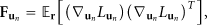
In practice, the localization performance at sensor n can be evaluated by the mean square error (MSE) of the adopted location estimator, namely $\mathrm{Tr}\hspace{0.17em}({\mathbf{F}}_{{\mathbf{u}}_n}^{-1})$ . Note that ${\mathbf{F}}_{{\mathbf{u}}_n}$ for the TDOA-based localization scheme has been derived in [17]. For the sake of self-consistency, we outline the derivation of ${\mathbf{F}}_{{\mathbf{u}}_n}$ in the following. Based on estimation theory, ${\mathbf{F}}_{{\mathbf{u}}_n}$ can be evaluated by [54]:

$\begin{array}{c}{\mathbf{F}}_{{\mathbf{u}}_n}={\mathbb{E}}_{\mathbf{r}}\left[\left({\nabla }_{{\mathbf{u}}_n}{L}_{{\mathbf{u}}_n}\right){\left({\nabla }_{{\mathbf{u}}_n}{L}_{{\mathbf{u}}_n}\right)}^T\right],\end{array}$

(3)

where ${𝔼}_{\mathbf{r}}(·)$ denotes the ensemble average with respect to $\mathbf{r}$ , and $L_{{\mathbf{u}}_n}$ is the log-likelihood function of $\mathbf{r}$ with respect to ${\mathbf{u}}_n$ :

$\begin{array}{c}{L}_{{\mathbf{u}}_n}=-\frac{\ln \left({\left(2\pi \right)}^M\det \left({𝚺}_{{\mathbf{u}}_n}\right)\right)+{\left(\mathbf{r}-{\mathbf{v}}_{{\mathbf{u}}_n}\right)}^T{𝚺}_{{\mathbf{u}}_n}^{-1}\left(\mathbf{r}-{\mathbf{v}}_{{\mathbf{u}}_n}\right)}{2}.\end{array}$

(4)

By some mathematical manipulations, we can show that:

$\begin{array}{c}{\mathbf{F}}_{{\mathbf{u}}_n}={\mathbf{\Phi }}_{{\mathbf{u}}_n}{𝚺}_{{\mathbf{u}}_n}^{-1}{\mathbf{\Phi }}_{{\mathbf{u}}_n}^T,\end{array}$

(5)

where ${\mathrm{\Phi }}_{{\mathbf{u}}_n}={\nabla }_{{\mathbf{u}}_n}({\mathbf{v}}_{{\mathbf{u}}_n}^T)$ is a $2\times M$ matrix with the mth column equal to $({\mathbf{u}}_n-{\mathbf{q}}_n)/(d_{n,{\mathbf{u}}_n})-({\mathbf{u}}_n-{\mathbf{p}}_m)/(D_{m,{\mathbf{u}}_n})$ . Using the matrix inversion formula $(\mathbf{J}+\mathbf{x}{\mathbf{y}}^T{)}^{-1}={\mathbf{J}}^{-1}-({\mathbf{J}}^{-1}\mathbf{x}{\mathbf{y}}^T{\mathbf{J}}^{-1})/(1+{\mathbf{y}}^T{\mathbf{J}}^{-1}\mathbf{x})$ , we can further reduce (5) to:

$\begin{array}{c}{\mathbf{F}}_{{\mathbf{u}}_n}={\mathbf{A}}_{{\mathbf{u}}_n}-{\eta }_{{\mathbf{u}}_n}{\mathbf{B}}_{{\mathbf{u}}_n},\end{array}$

(6)

where

$\begin{array}{c}{\mathbf{A}}_{{\mathbf{u}}_n}={\mathbf{\Phi }}_{{\mathbf{u}}_n}{\mathbf{\Lambda }}_{{\mathbf{u}}_n}^{-1}{\mathbf{\Phi }}_{{\mathbf{u}}_n}^T,\\ {\mathbf{B}}_{{\mathbf{u}}_n}=\left({\mathbf{\Phi }}_{{\mathbf{u}}_n}{\mathbf{\Lambda }}_{{\mathbf{u}}_n}^{-1}{\mathbf{1}}_M\right){\left({\mathbf{\Phi }}_{{\mathbf{u}}_n}{\mathbf{\Lambda }}_{{\mathbf{u}}_n}^{-1}{\mathbf{1}}_M\right)}^T,\\ {\eta }_{{\mathbf{u}}_n}=\frac{1}{f_{\text{a}\to \text{s}}{\left({ϵ}_n,d_{n,{\mathbf{u}}_n}\right)}^{-1}+{\mathbf{1}}_M^T{\mathbf{\Lambda }}_{{\mathbf{u}}_n}^{-1}{\mathbf{1}}_M}.\end{array}$

(7)

3.3. Impact of Ranging Energy on the MSE Performance

The MSE performance at sensor n can be evaluated by $\mathrm{Tr}\hspace{0.17em}({\mathbf{F}}_{{\mathbf{u}}_n}^{-1})={\lambda }_{{\mathbf{u}}_n,1}^{-1}+{\lambda }_{{\mathbf{u}}_n,2}^{-1}$ , where ${\lambda }_{{\mathbf{u}}_n,1}$ and ${\lambda }_{{\mathbf{u}}_n,2}$ denote the two eigenvalues of ${\mathbf{F}}_{{\mathbf{u}}_n}$ arranged in ascending order ( ${\lambda }_{{\mathbf{u}}_n,1}\le {\lambda }_{{\mathbf{u}}_n,2}$ ). First of all, we present the following theorems about the impact of ${ϵ}_n$ and $E_{\text{b}}$ on ${\lambda }_{{\mathbf{u}}_n,1}$ and ${\lambda }_{{\mathbf{u}}_n,2}$ .

Theorem 1.

Both ${\lambda }_{{\mathbf{u}}_n,1}$ and ${\lambda }_{{\mathbf{u}}_n,2}$ are nondecreasing when ${ϵ}_n$ increases.

Proof.

It is easy to see that ${\eta }_{{\mathbf{u}}_n}$ reduces as ${ϵ}_n$ increases, since $f_{\text{a}\to \text{s}}({ϵ}_n,d_{n,{\mathbf{u}}_n})$ is a decreasing function of ${ϵ}_n$ . Suppose ${ϵ}_n$ is increased by a small amount. As a consequence, ${\eta }_{{\mathbf{u}}_n}$ becomes ${\eta }_{{\mathbf{u}}_n}^{\prime }={\eta }_{{\mathbf{u}}_n}-\delta$ where δ is a positive value, while ${\mathbf{F}}_{{\mathbf{u}}_n}$ , ${\lambda }_{{\mathbf{u}}_n,1}$ , and ${\lambda }_{{\mathbf{u}}_n,2}$ become ${\mathbf{F}}_{{\mathbf{u}}_n}^{\prime }={\mathbf{F}}_{{\mathbf{u}}_n}+\delta {\mathbf{B}}_{{\mathbf{u}}_n}$ , ${\lambda }_{{\mathbf{u}}_n,1}^{\prime }$ , and ${\lambda }_{{\mathbf{u}}_n,2}^{\prime }$   ( ${\lambda }_{{\mathbf{u}}_n,1}^{\prime }\le {\lambda }_{{\mathbf{u}}_n,2}^{\prime }$ ), respectively. Apparently, ${\mathbf{B}}_{{\mathbf{u}}_n}$ is positive semidefinite, and therefore ${\lambda }_{{\mathbf{u}}_n,1}^{\prime }\ge {\lambda }_{{\mathbf{u}}_n,1}$ and ${\lambda }_{{\mathbf{u}}_n,2}^{\prime }\ge {\lambda }_{{\mathbf{u}}_n,2}$ hold according to [55, Corollary 4.3.3]. Therefore, both ${\lambda }_{{\mathbf{u}}_n,1}$ and ${\lambda }_{{\mathbf{u}}_n,2}$ are nondecreasing when ${ϵ}_n$ increases.

Theorem 2.

Both ${\lambda }_{{\mathbf{u}}_n,1}$ and ${\lambda }_{{\mathbf{u}}_n,2}$ are nondecreasing when $E_{\text{b}}$ increases.

Proof.

Suppose $E_{\text{b}}$ is reduced by a small amount to $E_{\text{b}}^{\prime }$ . As a consequence, ${\mathbf{\Sigma }}_{{\mathbf{u}}_n}$ , ${\mathbf{F}}_{{\mathbf{u}}_n}$ , ${\lambda }_{{\mathbf{u}}_n,1}$ , and ${\lambda }_{{\mathbf{u}}_n,2}$ become ${\mathbf{\Sigma }}_{{\mathbf{u}}_n}^{\prime }$ , ${\mathbf{F}}_{{\mathbf{u}}_n}^{\prime }$ , ${\lambda }_{{\mathbf{u}}_n,1}^{\prime }$ , and ${\lambda }_{{\mathbf{u}}_n,2}^{\prime }$   ( ${\lambda }_{{\mathbf{u}}_n,1}^{\prime }\le {\lambda }_{{\mathbf{u}}_n,2}^{\prime }$ ), respectively.

Let us define a series of matrices $\{{\mathbf{C}}_m{\}}_{m=0}^M$ , where ${\mathbf{C}}_0={\mathbf{\Sigma }}_{{\mathbf{u}}_n}$ , ${\mathbf{C}}_m={\mathbf{C}}_{m-1}+{\mathrm{\Delta }}_m{\mathbf{e}}_m{\mathbf{e}}_m^T$ , ${\mathrm{\Delta }}_m=(f_{\text{b}\to \text{a}}(E_{\text{b}}^{\prime },L_{m,n})+f_{\text{b}\to \text{s}}(E_{\text{b}}^{\prime },D_{m,{\mathbf{u}}_n}))-(f_{\text{b}\to \text{a}}(E_{\text{b}},L_{m,n})+f_{\text{b}\to \text{s}}(E_{\text{b}},D_{m,{\mathbf{u}}_n}))$ , and ${\mathbf{e}}_m$ is an $M\times 1$ all-zero column vector except for the mth entry which is equal to 1. Since both $f_{\text{b}\to \text{a}}(E_{\text{b}},L_{m,n})$ and $f_{\text{b}\to \text{s}}(E_{\text{b}},D_{m,{\mathbf{u}}_n})$ are decreasing functions of $E_{\text{b}}$ , ${\mathrm{\Delta }}_m$ is positive ( $1\le m\le M$ ).

Using the matrix inversion formula, we can show that $(1\le m\le M)$ :

$\begin{array}{c}{\mathbf{C}}_m^{-1}={\mathbf{C}}_{m-1}^{-1}-{\mu }_m{\mathbf{h}}_m{\mathbf{h}}_m^T,\end{array}$

(8)

where ${\mathbf{h}}_m={\mathbf{C}}_{m-1}^{-1}{\mathbf{e}}_m$ and ${\mu }_m=1/({\mathrm{\Delta }}_m^{-1}+{\mathbf{e}}_m^T{\mathbf{C}}_{m-1}^{-1}{\mathbf{e}}_m)$ .

We can see that ${\mathbf{C}}_M={\mathbf{\Sigma }}_{{\mathbf{u}}_n}^{\prime }$ . Using (8) successively, we can show that:

${𝚺}_{{\mathbf{u}}_n}^{\prime -1}={𝚺}_{{\mathbf{u}}_n}^{-1}-{\displaystyle \sum }_{m=1}^M{\mu }_m{\mathbf{h}}_m{\mathbf{h}}_m^T.$

(9)

Inserting (9) into (5), we can show that

$\begin{array}{c}{\mathbf{F}}_{{\mathbf{u}}_n}^{\prime }={\mathbf{F}}_{{\mathbf{u}}_n}-{\mathbf{D}}_{{\mathbf{u}}_n},\end{array}$

(10)

where ${\mathbf{D}}_{{\mathbf{u}}_n}={\sum }_{m=1}^M{\mu }_m({\mathrm{\Phi }}_{{\mathbf{u}}_n}{\mathbf{h}}_m)({\mathrm{\Phi }}_{{\mathbf{u}}_n}{\mathbf{h}}_m{)}^T$ .

Apparently, ${\mu }_m$ is positive, and thus ${\mathbf{D}}_{{\mathbf{u}}_n}$ is positive semidefinite. Therefore, ${\lambda }_{{\mathbf{u}}_n,1}^{\prime }\le {\lambda }_{{\mathbf{u}}_n,1}$ and ${\lambda }_{{\mathbf{u}}_n,2}^{\prime }\le {\lambda }_{{\mathbf{u}}_n,2}$ according to [55, Corollary 4.3.3]. This means that both ${\lambda }_{{\mathbf{u}}_n,1}$ and ${\lambda }_{{\mathbf{u}}_n,2}$ are unchanged or reduced as $E_{\text{b}}$ reduces. Equivalently, both ${\lambda }_{{\mathbf{u}}_n,1}$ and ${\lambda }_{{\mathbf{u}}_n,2}$ are unchanged or increased as $E_{\text{b}}$ increases. Therefore, both ${\lambda }_{{\mathbf{u}}_n,1}$ and ${\lambda }_{{\mathbf{u}}_n,2}$ are nondecreasing when $E_{\text{b}}$ increases.

Based on the above two theorems, $\mathrm{Tr}\hspace{0.17em}({\mathbf{F}}_{{\mathbf{u}}_n}^{-1})$ is nonincreasing as $E_{\text{b}}$ or ${ϵ}_n$ increases, which means that the MSE performance at sensor n does not degrade as $E_{\text{b}}$ or ${ϵ}_n$ increases.

3.4. Comments on the Assumptions

It is important to examine more closely the assumptions we made. First, the TOA estimates at the sensor and the anchor is unbiased and only degraded by the Gaussian-distributed TOA estimation error. However, this might not be true for practical TOA estimators. Second, each anchor can measure $t_{{\mathbf{q}}_n}$ precisely with its internal clock, which implies that each anchor can perform perfect calibration. In reality, this is rarely achieved. Third, the location estimate is unbiased and achieves the CRB. In practice, it is hard to implement a CRB achieving location estimator by a sensor with limited capability of computation.

Our assumptions are motivated by the fact that if we make more realistic assumptions, it is generally very difficult to derive the localization performance analytically. Although our assumptions seem too optimistic in practice, the derived performance has an attractive structure which not only facilitates mathematical analysis, but also lends the ranging energy optimization problems proposed in Section 4 to be efficiently solved. Furthermore, the optimal ranging energy for a more realistic scenario is actually lower bounded by the results computed for the optimistic scenario assumed here. Therefore, our assumptions lead to useful optimization results, which not only can be computed efficiently, but also provide a sense of how much energy should be allocated at least.

Note that it is very attractive to investigate the gap between the optimal energy computed under our assumptions and that for real scenarios, when more knowledge is available about the statistics of the signal queuing and the implemented location estimator. Intuitively, this gap should be translated from the localization performance loss due to the impairments present in a real scenario but ignored by our assumptions. This topic is part of our future work.

4. Ranging Energy Optimization

4.1. RSP Requirements and Constraints

The RSP over the service area $S_n$ requires that for all ${\mathbf{u}}_n\in S_n$ , $\parallel {\widehat{\mathbf{u}}}_n-{\mathbf{u}}_n{\parallel }_2$ should be smaller than $R_{\text{e}}$ with probability higher than $P_{\text{e}}$ . To achieve the RSP over $S_n$ , we adopt the constraint developed in [47]:

${\lambda }_n\ge {\lambda }_{\text{th}},$

(11)

where ${\lambda }_n={\min \hspace{0.17em}}_{{\mathbf{u}}_n\in S_n}{\lambda }_{{\mathbf{F}}_{{\mathbf{u}}_n}}$ , with ${\lambda }_{{\mathbf{F}}_{{\mathbf{u}}_n}}$ and ${\lambda }_{\text{th}}$ denoting the minimal eigenvalue of ${\mathbf{F}}_{{\mathbf{u}}_n}$ and a threshold eigenvalue, respectively. Specifically, ${\lambda }_{\text{th}}=-2R_{\text{e}}^{-2}\ln \hspace{0.17em}(1-P_{\text{e}})$ if ${\widehat{\mathbf{u}}}_n$ is Gaussian distributed, and ${\lambda }_{\text{th}}=2R_{\text{e}}^{-2}(1-P_{\text{e}}{)}^{-1}$ if ${\widehat{\mathbf{u}}}_n$ has an unknown distribution. We can easily find that the ${\lambda }_{\text{th}}$ associated with the Gaussian distributed ${\widehat{\mathbf{u}}}_n$ is smaller than the one corresponding to the ${\widehat{\mathbf{u}}}_n$ with an unknown distribution.

To achieve the RSP over all service areas, the RSP constraint to be satisfied is $\lambda ={\min \hspace{0.17em}}_{n\in \{1,\dots ,N\}}{\lambda }_n\ge {\lambda }_{\text{th}}$ , or equivalently for all $n\in \{1,\dots ,N\}$ , ${\lambda }_n\ge {\lambda }_{\text{th}}$ . We can see that ${\lambda }_n$ and λ play key roles in judging if the RSP is achieved over all service areas. We present the following theorems regarding the impact of ${ϵ}_n$ and $E_{\text{b}}$ on ${\lambda }_n$ and λ.

Theorem 3.

For all $n\in \{1,\dots ,N\}$ , ${\lambda }_{\text{n}}$ is nondecreasing when either ${ϵ}_n$ or $E_{\text{b}}$ increases.

Proof.

Suppose ${ϵ}_n$ is increased to ${ϵ}_n^{\prime }$ . As a result, ${\lambda }_{{\mathbf{F}}_{{\mathbf{u}}_n}}$ and ${\lambda }_n$ become ${\lambda }_{{\mathbf{F}}_{{\mathbf{u}}_n}}^{\prime }$ and ${\lambda }_n^{\prime }$ , respectively. Let's say ${\lambda }_n^{\prime }={\lambda }_{{\mathbf{F}}_{{\mathbf{y}}_n}}^{\prime }$ , where ${\mathbf{y}}_n$ denotes a position within $S_n$ . According to Theorem 1, ${\lambda }_{{\mathbf{F}}_{{\mathbf{y}}_n}}^{\prime }\ge {\lambda }_{{\mathbf{F}}_{{\mathbf{y}}_n}}$ . Since ${\lambda }_{{\mathbf{F}}_{{\mathbf{y}}_n}}\ge {\lambda }_n$ , we obtain ${\lambda }_n^{\prime }\ge {\lambda }_n$ , which means that ${\lambda }_n$ is nondecreasing when ${ϵ}_n$ increases. In a similar way, we can show that ${\lambda }_n$ is nondecreasing as well when $E_{\text{b}}$ increases.

Theorem 4.

λ is nondecreasing when any one of $\{{ϵ}_n{\}}_{n=1}^N$ or $E_{\text{b}}$ increases.

Proof.

Suppose any one of the anchors increases its ranging energy, say ${ϵ}_n$ , to be ${ϵ}_n^{\prime }$ . As a result, ${\lambda }_{{\mathbf{F}}_{{\mathbf{u}}_n}}$ and λ become ${\lambda }_{{\mathbf{F}}_{{\mathbf{u}}_n}}^{\prime }$ and ${\lambda }^{\prime }$ , respectively. Let's say ${\lambda }^{\prime }={\lambda }_{{\mathbf{F}}_{{\text{z}}_j}}^{\prime }$ , where ${\mathbf{z}}_j$ denotes a position within the service area $S_j$   ( $1\le j\le N$ ). According to Theorem 1, ${\lambda }_{{\mathbf{F}}_{{\mathbf{z}}_j}}^{\prime }\ge {\lambda }_{{\mathbf{F}}_{{\mathbf{z}}_j}}$ . Since ${\lambda }_{{\mathbf{F}}_{{\mathbf{z}}_j}}\ge \lambda$ , we obtain ${\lambda }^{\prime }\ge \lambda$ , which means that λ is nondecreasing when ${ϵ}_n$ increases. In a similar way, we can show that λ is nondecreasing as well when $E_{\text{b}}$ increases.

According to the above theorems, the RSP over all service areas may be achieved by enhancing the ranging energy of the beacons or the anchors. We will proceed with the related ranging energy optimization problems in the following subsections.

4.2. Anchor Ranging Energy Optimization

The first ranging energy optimization problem we consider is to find the lowest ranging energy ${ϵ}_n^{\text{o}}$ for each anchor given the prescribed beacon ranging energy so that the RSP over all service areas is fulfilled.

It is important to note that $R_{\text{e}}$ and $P_{\text{e}}$ should be prescribed so that it is possible to satisfy $\lambda \ge {\lambda }_{\text{th}}$ when ${ϵ}_n\le {ϵ}_n^{\text{U}}$ , for all n and $E_{\text{b}}$ has a prescribed value between $E_{\text{b}}^{\text{L}}$ and $E_{\text{b}}^{\text{U}}$ . To this end, we first compute λ using the prescribed value for $E_{\text{b}}$ and ${ϵ}_n={ϵ}_n^{\text{U}}$ , for all n with the numerical method described in Section 4.4. We denote this λ by ${\lambda }_{\text{A}}$ , which is an upper bound for λ according to Theorem 4 when ${ϵ}_n\le {ϵ}_n^{\text{U}}$ , for all n and $E_{\text{b}}$ takes the prescribed value. Apparently, $R_{\text{e}}$ and $P_{\text{e}}$ should be prescribed with ${\lambda }_{\text{th}}\le {\lambda }_{\text{A}}$ satisfied, so that there exists a solution for the considered problem.

Since ${\lambda }_n$ is nondecreasing as ${ϵ}_n$ increases according to Theorem 3, we can use the bisection method to find ${ϵ}_n^{\text{o}}$ for each anchor individually so that the RSP constraint is fulfilled over each cell. Specifically, the proposed algorithm for finding ${ϵ}_n^{\text{o}}$ is depicted in Algorithm 1. Note that the energy optimization for every anchor is independent of the others, and the bisection method has a complexity of $O({\log \hspace{0.17em}}_2(\mathrm{\Delta }))$ , where $\mathrm{\Delta }$ is the length of the interval where the optimization variable lies [56]. Therefore, the complexity of Algorithm 1 is $O(N{\log \hspace{0.17em}}_2({ϵ}_{\text{U}}-{ϵ}_{\text{L}}))$ , which means that Algorithm 1 has a good scalability for large WSNs since the number of searches required increases linearly with respect to the number of anchors.

Algorithm 1: Optimization algorithm for computing ${ϵ}_n^o$ .

Initialization: ${ϵ}_{\text{U}}={ϵ}_n^{\text{U}}$ ; ${ϵ}_{\text{L}}={ϵ}_n^{\text{L}}$ ;

 while ${ϵ}_{\text{U}}-{ϵ}_{\text{L}}>0$   do

   ${ϵ}_{\text{M}}=({ϵ}_{\text{U}}+{ϵ}_{\text{L}})/2$ ;

  Compute ${\lambda }_n$ when ${ϵ}_n={ϵ}_{\text{M}}$ with the numerical

  method described in Section 4.4;

  if ${\lambda }_n<{\lambda }_{\text{th}}$   then

    ${ϵ}_{\text{L}}={ϵ}_{\text{M}}$ ;

  else if ${\lambda }_n>{\lambda }_{\text{th}}$   then

    ${ϵ}_{\text{U}}={ϵ}_{\text{M}}$ ;

  else

   Go to Output;

  end if

 end while

Output: ${ϵ}_n^{\text{o}}={ϵ}_{\text{M}}$ .

4.3. Beacon Ranging Energy Optimization

The second ranging energy optimization problem we consider is to find the lowest beacon ranging energy $E_{\text{b}}^{\text{o}}$ given the prescribed anchor ranging energy so that the RSP over all service areas is fulfilled.

First of all, it is important to note that $R_{\text{e}}$ and $P_{\text{e}}$ should be prescribed so that it is possible to satisfy the RSP constraint $\lambda \ge {\lambda }_{\text{th}}$ when $E_{\text{b}}\le E_{\text{b}}^{\text{U}}$ and ${ϵ}_n$ has a prescribed value between ${ϵ}_n^{\text{L}}$ and ${ϵ}_n^{\text{U}}$ , for all $n\in \{1,\dots ,N\}$ . To this end, we first compute λ using the prescribed values for $\{{ϵ}_n{\}}_{n=1}^N$ and $E_{\text{b}}=E_{\text{b}}^{\text{U}}$ with the numerical method described in Section 4.4. We denote this λ by ${\lambda }_{\text{B}}$ , which is an upper bound for λ according to Theorem 4 when $E_{\text{b}}\le E_{\text{b}}^{\text{U}}$ and $\{{ϵ}_n{\}}_{n=1}^N$ take prescribed values. Apparently, $R_{\text{e}}$ and $P_{\text{e}}$ should be prescribed with ${\lambda }_{\text{th}}\le {\lambda }_{\text{B}}$ satisfied, so that there exists a solution for the considered problem.

Since λ is nondecreasing as $E_{\text{b}}$ increases according to Theorem 4, we can use the bisection method to find $E_{\text{b}}^{\text{o}}$ . Specifically, the proposed algorithm is depicted in Algorithm 2. Note that the complexity of Algorithm 2 is $O({\log \hspace{0.17em}}_2(E_{\text{U}}-E_{\text{L}}))$ .

Algorithm 2: Optimization algorithm for computing $E_b^o$ .

Initialization: $E_{\text{U}}=E_{\text{b}}^{\text{U}}$ ; $E_{\text{L}}=E_{\text{b}}^{\text{L}}$ ;

 while $E_{\text{U}}-E_{\text{L}}>0$   do

   $E_{\text{M}}=(E_{\text{U}}+E_{\text{L}})/2$ ;

  Compute λ when $E_{\text{b}}=E_{\text{M}}$ with the numerical

  method described in Section 4.4;

  if $\lambda <{\lambda }_{\text{th}}$   then

    $E_{\text{L}}=E_{\text{M}}$ ;

  else if $\lambda >{\lambda }_{\text{th}}$   then

    $E_{\text{U}}=E_{\text{M}}$ ;

  else

   Go toOutput;

  end if

 end while

Output: $E_{\text{b}}^{\text{o}}=E_{\text{M}}$ .

4.4. Numerical Issues Related to the Proposed Algorithms

In general, the service areas are continuous. To compute $\{{\lambda }_{\text{A}},{ϵ}_n^{\text{o}}\}$ and $\{{\lambda }_{\text{B}},E_{\text{b}}^{\text{o}}\}$ numerically, we uniformly sample a set of grid points $G_n=\{g_{n,k}{\}}_{k=1}^{K_n}$ in $S_n$ , $\text{for}\mathrm{\hspace{0.17em}\hspace{0.17em}}\text{all}\mathrm{\hspace{0.17em}\hspace{0.17em}}n$ , and compute ${\lambda }_n$ through the approximation ${\lambda }_n\approx {\min \hspace{0.17em}}_{{\mathbf{u}}_n\in G_n}{\lambda }_{{\mathbf{F}}_{{\mathbf{u}}_n}}$ wherever needed. The numerically computed $\{{\lambda }_{\text{A}},{ϵ}_n^{\text{o}}\}$ and $\{{\lambda }_{\text{B}},E_{\text{b}}^{\text{o}}\}$ are actually associated with fulfilling the RSP constraints over $\{G_n{\}}_{n=1}^N$ instead of $\{S_n{\}}_{n=1}^N$ .

On the one hand, the numerically computed ${\lambda }_n$ is an upper bound on the true value of ${\lambda }_n$ , since the minimization is performed numerically over $G_n$ which is a subset of $S_n$ . As a result, the numerically computed λ is an upper bound on the true value of λ, and therefore the numerically computed ${\lambda }_{\text{A}}$ and ${\lambda }_{\text{B}}$ are upper bounds for their true values.

On the other hand, the numerically computed ${ϵ}_n^{\text{o}}$ , for all n is a lower bound on its true value, since the set of ${ϵ}_n$ 's enabling the RSP over $S_n$ is a subset of the ${ϵ}_n$ 's that enables the RSP over $G_n$ . In addition, the numerically computed $E_{\text{b}}^{\text{o}}$ is a lower bound on its true value, since the set of $E_{\text{b}}$ 's enabling the RSP over $\{S_n{\}}_{n=1}^N$ is a subset of the $E_{\text{b}}$ 's that enables the RSP over $\{G_n{\}}_{n=1}^N$ .

Note that each of the numerically computed ${\lambda }_{\text{A}}$ , ${ϵ}_n^{\text{o}}$ , ${\lambda }_{\text{B}}$ , and $E_{\text{b}}^{\text{o}}$ approaches its true value associated with the original continuous service areas as the sampling spacing approaches zero, and the numerical results are reasonable approximations if the sampling spacing is sufficiently small. In practice, we can reduce the sampling spacing gradually, and compute the numerical results for each sampling spacing. When further reducing the sampling spacing results in a tolerably small change of the numerical results, we can adopt these numerical results as the final solutions.

5. Numerical Experiments

5.1. Description of an Illustrative Sensor Positioning System

For the numerical experiments, we consider an illustrative sensor positioning system shown in Figure 3. There exist 3 beacons located at ${\mathbf{p}}_1=[-\mathrm{2,2}{]}^T$ , ${\mathbf{p}}_2=[\mathrm{2,2}{]}^T$ , and ${\mathbf{p}}_3=[0,-2{]}^T$ , respectively. There are two anchors located at ${\mathbf{q}}_1=[-\mathrm{1,0}{]}^T$ and ${\mathbf{q}}_2=[\mathrm{1,0}{]}^T$ , respectively. We assume $S_1=\{{\mathbf{u}}_1\hspace{0.17em}|\hspace{0.17em}0.2\le \parallel {\mathbf{u}}_1-{\mathbf{q}}_1{\parallel }_2\le 1\}$ , and $S_2=\{{\mathbf{u}}_2\hspace{0.17em}|\hspace{0.17em}0.2\le \parallel {\mathbf{u}}_2-{\mathbf{q}}_2{\parallel }_2\le 1\}$ . Note that the unit for all the aforementioned values related to coordinates or length is meter.

Figure 3

An illustrative system setup where the yellow area surrounding each anchor represents the associated service area.

For the considered system, a line-of-sight (LOS) channel exists between any two nodes of the set consisting of sensor n, anchor n, and beacon m, for all $m\in \{1,\dots ,M\}$ , for all $n\in \{1,\dots ,N\}$ . In addition, this LOS channel incurs a propagation delay $d/c$ and a path loss $\alpha d^{-\beta }$ , where d is the propagation distance of this channel, c stands for the signal propagation speed, α represents the path gain at 1 m, and β denotes the path loss exponent. Each channel remains unchanged during the localization process.

The two-sided power spectral density of the additive white Gaussian noise (AWGN) at sensor n and anchor n is equal to $N_{\text{s}}/2$ . Each TOA estimate is Gaussian distributed and achieves the associated CRB, which has been derived in [47]. Using the formulas given in [47], we can show that $f_{\text{a}\to \text{s}}({ϵ}_n,d_{n,{\mathbf{u}}_n})=c^2{N}_{\text{s}}/(2\alpha d_{n,{\mathbf{u}}_n}^{-\beta }{\omega }_{\text{a},n}^2{ϵ}_n)$ , $f_{\text{b}\to \text{s}}(E_{\text{b}},D_{m,{\mathbf{u}}_n})=c^2{N}_{\text{s}}/(2\alpha D_{m,{\mathbf{u}}_n}^{-\beta }{\omega }_{\text{b}}^2{E}_{\text{b}})$ , and $f_{\text{b}\to \text{a}}(E_{\text{b}},L_{m,n})$ = $c^2{N}_{\text{s}}/(2\alpha L_{m,n}^{-\beta }{\omega }_{\text{b}}^2{E}_{\text{b}})$ , Here, ${\omega }_{\text{a},n}$ and ${\omega }_{\text{b}}$ are respectively the root-mean-square (RMS) angular frequency of $s_{\text{a},n}(t)$ and $s_{\text{b}}(t)$ :

$\begin{array}{cc}\hfill {\omega }_{\text{a},n}& =\sqrt{\frac{{\int }_{-\infty }^{+\infty }{\left|2\pi f{S}_{\text{a},n}\left(f\right)\right|}^{2}df}{{\int }_{-\infty }^{+\infty }{\left|S_{\text{a},n}\left(f\right)\right|}^{2}df}},\hfill \\ \hfill {\omega }_{\text{b}}& =\sqrt{\frac{{\int }_{-\infty }^{+\infty }{\left|2\pi f{S}_{\text{b}}\left(f\right)\right|}^{2}df}{{\int }_{-\infty }^{+\infty }{\left|S_{\text{b}}\left(f\right)\right|}^{2}df}},\hfill \end{array}$

(12)

where $S_{\text{a},n}(f)$ and $S_{\text{b}}(f)$ represent the spectrum of $s_{\text{a},n}(t)$ and $s_{\text{b}}(t)$ , respectively.

The parameters are set as $\alpha =1$ , $\beta =2$ , ${\omega }_{\text{b}}/2\pi ={\omega }_{\text{a},n}/2\pi =1$  GHz, for all n, $N_{\text{s}}=1$  W/Hz, $c=3\times 10^8$  m/s. We assume every ranging signal can be received reliably by a sensor or an anchor if the received energy is above $E_{\text{t}}=0$  dBJ. We can find that $d_1={\max \hspace{0.17em}}_{{\mathbf{u}}_1\in S_1}\parallel {\mathbf{u}}_1-{\mathbf{q}}_1{\parallel }_2=1$  m, $d_2={\max \hspace{0.17em}}_{{\mathbf{u}}_2\in S_2}\parallel {\mathbf{u}}_2-{\mathbf{q}}_2{\parallel }_2=1$  m, and $d_3={\max \hspace{0.17em}}_{m\in \{\mathrm{1,2},3\},{\mathbf{u}}_n\in S_1\cup S_2}\parallel {\mathbf{u}}_n-{\mathbf{p}}_m{\parallel }_2=(\sqrt{13}+1)$  m. As a result, we set ${ϵ}_1^{\text{L}}=E_{\text{t}}/(\alpha {d_1}^{-\beta })=0$  dBJ, ${ϵ}_2^{\text{L}}=E_{\text{t}}/(\alpha {d_2}^{-\beta })=0$  dBJ, and $E_{\text{b}}^{\text{L}}=E_{\text{t}}/(\alpha {d_3}^{-\beta })=13.27$  dBJ, so that every ranging signal can be received reliably by a sensor or an anchor.

5.2. Numerical Results

For the RSP constraint, we prescribe $P_{\text{e}}$ to be fixed at 0.8. As $R_{\text{e}}$ increases from 1 cm to 10 cm, ${\lambda }_{\text{th}}$ is shown in Figure 4 when the position estimate has a Gaussian distribution and an unknown distribution, respectively. We can see that the ${\lambda }_{\text{th}}$ corresponding to the unknown distribution is much greater than the one associated with the Gaussian distribution.

Figure 4

${\lambda }_{\text{th}}$ with respect to $R_e$ when the position estimate has a Gaussian distribution and an unknown distribution, respectively.

For the numerical experiments, we find that uniform spacing equal to 2 cm is sufficiently small for sampling $S_1$ and $S_2$ , respectively, to produce $G_1$ and $G_2$ , since a further reduction of the spacing leads to a negligible change of the numerical results.

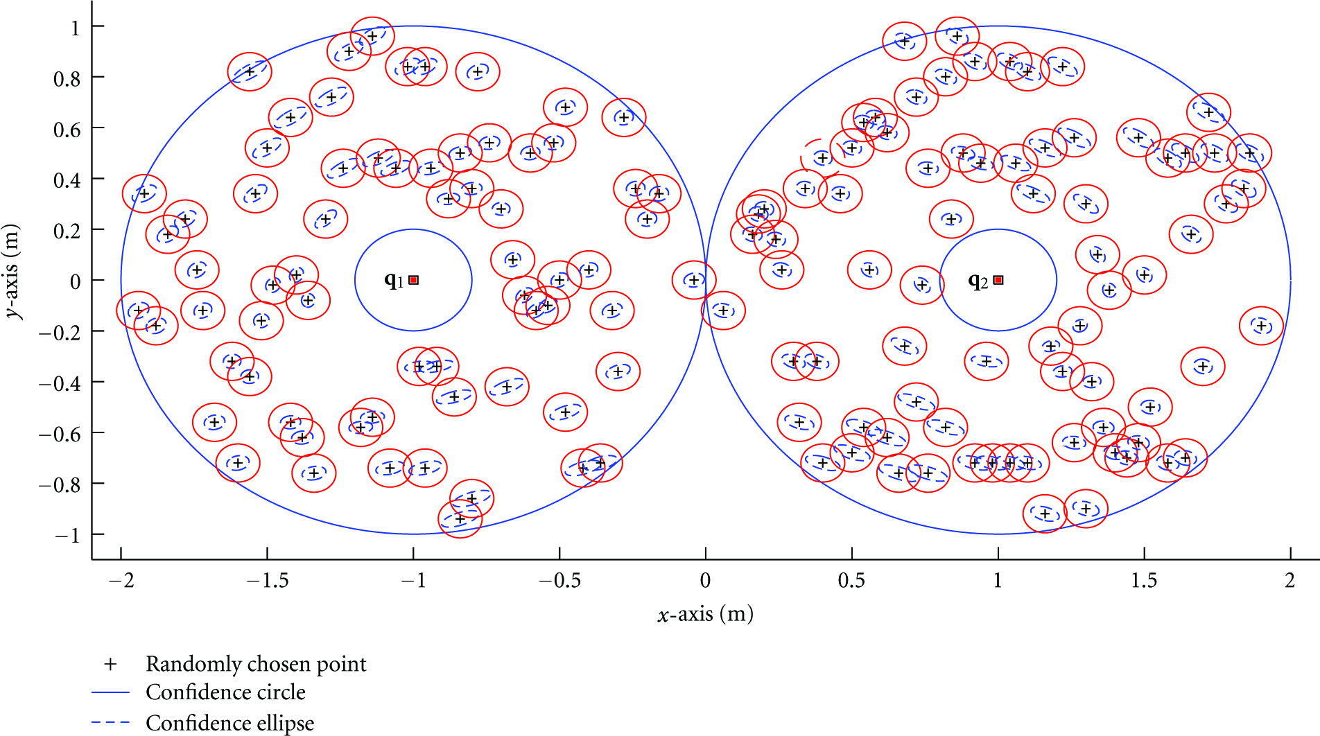
We first consider the anchor ranging energy optimization when $E_{\text{b}}=20$  dBJ and ${ϵ}_1^{\text{U}}={ϵ}_2^{\text{U}}=5$  J. The numerically computed ${\lambda }_{\text{A}}$ is equal to 33.15 dB. We prescribe $R_{\text{e}}$ to be 7.2 cm which corresponds to ${\lambda }_{\text{th}}=27.93$  dB when the position estimate has a Gaussian distribution. Using Algorithm 1, the numerically computed ${ϵ}_1^{\text{o}}$ and ${ϵ}_2^{\text{o}}$ are both equal to ${ϵ}_2^{\text{L}}={ϵ}_2^{\text{L}}=0$  dBJ. This means that the lowest ${ϵ}_1$ and ${ϵ}_2$ satisfying the RSP in all service areas are no greater than ${ϵ}_1^{\text{L}}$ and ${ϵ}_2^{\text{L}}$ , respectively. To justify the effectiveness of these values for the RSP, we randomly choose a set of positions within $S_1$ and $S_2$ . Centered at each selected position, the circle of radius $R_{\text{e}}$ as well as the confidence ellipse in which the location estimate falls with probability $P_{\text{e}}$ are plotted in Figure 5. It is shown that each confidence ellipse is contained in the corresponding circle, which means that the accuracy requirement is fulfilled at each selected position. When the position estimate has an unknown distribution, we find that ${\lambda }_{\text{th}}=32.85$  dB, and the numerically computed ${ϵ}_1^{\text{o}}$ and ${ϵ}_2^{\text{o}}$ are both equal to 3.16 dBJ. This increase of each anchor's ranging energy from 0 dBJ to 3.16 dBJ represents the extra anchor ranging energy required to compensate for the unavailable knowledge about the distribution of the sensor's position estimate when $E_{\text{b}}=20$  dBJ.

Figure 5

Confidence ellipses and circles for randomly chosen positions when $E_{\text{b}}=20$  dBJ and ${ϵ}_1^{\text{o}}={ϵ}_2^{\text{o}}=0$  dBJ.

We then consider the beacon ranging energy optimization when ${ϵ}_1={ϵ}_2=1$  dBJ and $E_{\text{b}}^{\text{U}}=20$  dBJ, for which the numerically computed ${\lambda }_{\text{B}}$ is equal to 32.65 dB. We prescribe $R_{\text{e}}$ to be 7.5 cm which corresponds to ${\lambda }_{\text{th}}=27.58$  dB when the position estimate is Gaussian distributed. Using Algorithm 2, $E_{\text{b}}^{\text{o}}$ is numerically computed as 14.53 dBJ. To justify the effectiveness of these values for the RSP, we randomly choose a set of positions within $S_1$ and $S_2$ , and then plot in Figure 6 the circle of radius $R_{\text{e}}$ as well as the confidence ellipse of probability $P_{\text{e}}$ centered at each selected position. Since each confidence ellipse is contained in the corresponding circle, the accuracy requirement is fulfilled at each selected position. We find that ${\lambda }_{\text{th}}=32.50$  dB and $E_{\text{b}}^{\text{o}}=19.83$  dBJ when the position estimate has an unknown distribution. The increase of the beacon's ranging energy from 14.53 dBJ to 19.83 dBJ represents the extra beacon ranging energy required to compensate for the unavailable knowledge about the distribution of the sensor's position estimate when ${ϵ}_1={ϵ}_2=1$  dBJ.

Figure 6

Confidence ellipses and circles for randomly chosen positions when $E_{\text{b}}^{\text{o}}=14.53$  dBJ and ${ϵ}_1={ϵ}_2=1$  dBJ.

6. Conclusions

We have proposed a distributed localization scheme for an asynchronous WSN consisting of at least two beacons as well as some anchors, each collaborating with the beacons to help the sensors within the corresponding service area for self-localization. Most interestingly, each sensor does not need to emit either ranging or communication signals to neighbor sensors in the proposed scheme. Instead, each sensor only needs to estimate the time-of-arrivals (TOAs) of incoming ranging signals from the beacons and the anchors, and then the time-difference-of-arrival (TDOA) between the signal propagating from each beacon to the sensor and the one from that beacon to the sensor via an associated anchor is produced and converted to a range difference measurement at the sensor for self-localization. Assuming the location estimator adopted achieves the associated CRB, the localization performance at each sensor has been derived and analyzed. We have also considered ranging energy optimization problems related to the beacons and the anchors, when the system features robust performance in that a prescribed accuracy requirement is fulfilled in all service areas of the anchors. Practical algorithms have been presented to solve them, and the effectiveness of those algorithms has been illustrated by numerical experiments.