CFD Investigation on 3-Dimensional Interference of a Five-Hole Probe in an Automotive Wheel Arch

Abstract

Detailed flow measurements are essential for analysing flow structures found in confined spaces, particularly in various automotive applications. These measurements will be extremely helpful in solving flow dependent complexities. Although considerable progress has been made in computational techniques for investigating such flows, experimental flow measurements are still very difficult to carry out therein. Flows mapped using an array of robust instruments like multi-hole pressure probes can provide significant insight into the flow field of such complex flows. Pressure probes can withstand the harsh environments found in such applications; however being intrusive devices significant interference in flow field can limit their applicability. This paper presents an investigation of three-dimensional interference caused by multi-hole pressure probes in an automotive wheel arch. It involves simulation of flow around a pressure probe inserted at various locations within the wheel/wheel arch gap. Pressure and velocity fields along longitudinal and lateral planes have been mapped and the extent of interference caused by the probe along three orthogonal axes has been presented. A three-dimensional ellipsoid of interference has been defined to assist in recommending optimal placement of probes and minimise the error due to interprobe interaction, thus enhancing the measurement accuracy of transient flow phenomena.

1. Introduction

Multi-hole pressure probes are effective tools for multidimensional flow field measurements. They provide knowledge of flow velocity, direction, as well as total and static pressures at the point of interrogation. They require infrequent calibration and are fairly robust, which allows their use for flow metrology in harsh conditions like solid-liquid slurries [4] and inside axial compressors [5].

Most intrusive measuring devices like hot-wire anemometers are not robust enough to withstand the harsh environment inside regions like compressors, machines, and automotive wheel housings [6]. Nonintrusive measurement techniques like particle image velocimetry (PIV) and laser Doppler anemometry (LDA) require controlled environment and have very limited scope for online measurement during field tests. They also require direct line of sight from the interrogation area/point. One of the possible alternatives is to use multi-hole pressure probes by inserting them into the region to be mapped. Several applications in flow metrology require detailed flow maps of difficult-to-reach regions. These include flow measurements inside automotive wheel arches for analysis of flow around the rotating wheels. The flow in such regions has been found to be unsteady [1, 7–9]. It is seen in literature that lack of knowledge of flow variables in the flow field around rotating components like disc brakes causes limitations in their analysis to estimate cooling behaviour [10]. In situ measurements of flow around ventilated disc-brake rotors can also provide a huge amount of information on their cooling properties, and thus help alleviate brake noise and judder. Real-time measurement or flow mapping during field tests of even small areas with a single instrument can take several days to complete. In such situations it is essential to use arrays of multiple instruments. This will benefit in reducing not only testing time but also uncertainty errors which may arise due to low repeatability of field tests. Moreover multiple instruments positioned in key locations of the region being investigated will allow transient analysis of unsteady structures in the flow. Thus, a series of such instruments can be used in combination for detailed flow mapping in complex applications such as flow analysis in and around automobile wheel housing discussed earlier. Such data can be used to further investigate the nonuniformity of the overall flow field of the vehicle caused by the wheel and wheel arch. Quantification of this nonuniformity can be further used to study the effect on the overall forces and moments, and consequently the stability of road vehicles in nonuniform conditions like cross winds.

For accurate measurement of flow variables at each point, it is important that these probes cause least interference to the flow field under study and do not affect nearby probes. Flow field disturbance caused by pressure probes has been a major concern in their application [11]. Although advanced machining resources are now available, reducing the size of probe head is not the direct solution for optimising probe design. Decreasing the probe head diameter past 0.2 mm yields unacceptable response times of the pressure taps [11], thus preventing their use in unsteady applications.

Modification of the flow field of one probe by another may cause errors in pressure readings at the individual taps, resulting in inaccurate flow measurements. Although full three-dimensional calibration techniques for multi-hole pressure probes are now common practice [12, 13], this problem cannot be resolved by including standard correction factors for interprobe interaction in the calibration process. Optimum probe design will enhance accuracy of calibration and flow measurement by reducing such interference. Various probe head geometries have been discussed by Bryer and Pankhurst [12]; however a detailed analysis of the flow field interference caused by pressure probes is required for effective flow mapping using instrument arrays.

Multi-hole pressure probes have been used in applications where space is limited, such as downstream of the rotor in axial compressors [5]. Coldrick et al. [5] studied the influence of a four-hole probe on the flow between two stator blades as well as that of the proximity of the stator blades to the probe by performing computational fluid dynamic (CFD) analysis. It was found that the wake formed by the probe and the change in pressure distribution around the probe caused significant blockage. This affected the mass flow rate through the space between two blades containing the probe. Further work is required to correctly model numerous probes in more than one space between stator blades. Proximity of the probe to the stator blade leading the flow field has been shown to cause erroneous readings on the adjacent probe pressure port (tap).CFD techniques are extensively being used to establish the pressure probe calibration and interference. Seshadri et al. [14] analysed the effect of various body shapes on the annubar factor of averaging Pitot tubes by using computational techniques. The elliptical shape was found to have a minimum permanent pressure loss. The primary contributing factor for this lower pressure loss was found to be the rounding of edges. This also improved the performance of diamond-shaped annubars. Singh et al. [15] studied the effect of Reynolds number and upstream velocity profile on probe factor of a self-averaging Pitot tube. However the investigations were limited to a microbar tested in circular ducts. It was found that the Reynolds number and nonuniformity in the upstream velocity profile had little effect on the probe factor. The permanent pressure loss due to the probe was found to be of the order of the average dynamic pressure of the flow in the pipe. Malviya et al. [3] investigated the spatial extent of the interference caused by a five-hole probe. The probe was orientated such that the angle between the measuring axis and the free-stream flow was 0°. It was found that probe modified the flow in its immediate vicinity. This influence of the probe on the flow extended up to 5 times the diameter upstream and up to 13 times the diameter downstream. The transverse (lateral and vertical) components of velocity were found to be less than 1% of the free-stream velocity beyond these points. The analysis was however limited only to one dimension in the streamwise direction.

The above discussion shows that not much work has been done to systematically quantify the three-dimensional interference caused by multi-hole pressure probes or similar instruments to the flow field. It can also be seen that there is very little information available in literature about the optimum spacing of such intrusive measuring instruments in small spaces. One such area of interest is the wheel cavity in automotive applications. Although considerable progress has been made in understanding the overall flow field of road vehicles by using tools like wind tunnels as well as CFD little progress has been made in understanding transient flow field within the wheel cavity. It has been reported that the contribution of wheels to the overall drag of streamlined cars accounts for as much as 50% [16]. Detailed investigation of flow variables is required to quantify the effect of various geometric parameters of the wheel and wheel arch on various aspects such as brake cooling as well as forces and moments acting on the wheels and hence overall stability of vehicles.

Several attempts have been made to analyse the flow field around rotating as well as stationary wheels [7, 8, 17–21]. Research groups have tried to study the flow field around isolated wheels as well as those enclosed by wheel housings [1, 2, 7, 9]. Fackrell and Harvey [17] investigated two profiles of an isolated wheel with a focus on flow features around the wheel. The difference in flow field around stationary and rotating wheels was highlighted. Lift and drag were computed from pressure distributions over the wheels. However the scope of the work was limited to isolated wheels and the effect of rotation on lift, drag, and pressure distribution. Oswald and Browne [6] investigated the air flow velocity, direction, and turbulence levels around a passenger car tyre. Field tests were conducted using hot-wire anemometers and yarn tufts for velocity measurements and flow visualization, respectively. The effect of the air flow field on the tyre power loss was the focus of this work. However since hot-wire anemometers were the only flow instruments, the pressure distribution in the wheel arch was unknown. Moreover the hot-wire anemometers were prone to constant breakage as they are fragile instruments. Fabijanic [2] also investigated the effect of wheel and wheel well (cavity) on the overall lift and drag characteristics of road vehicles. Wind tunnel tests were conducted on a generic single-axle automotive body shape model. Dimensions of wheel and wheel wells encompassed wheel to wheel-well relationships for a wide range of vehicle types. It was shown that the addition of wheel and wheel-wells increased both drag and lift of the overall body by up to 90% and 67%, respectively, for various wheel and wheel-well relationships. It was also shown that the overall drag was primarily influenced by the wheel radius and the lift was influenced by the wheel-well depth. Surface pressure measurements and oil flow visualisations clearly indicated that the influence of the wheel and wheel wells on the overall drag and lift was caused due to the modification of the overall body flow by the wheels and wheel-wells. It was also found that the jetting produced at the wheel-ground contact point greatly influences the overall lift as it tends to interfere with the under-body flow. However there were errors introduced by the external strut assembly holding the wheel inside the wheel arch. Moreover pressure measurements were limited to a number of points on the inner surface of wheel arch. Flow field data inside the wheel/wheel-arch was not recorded.

Brake noise and brake fade are two major problems associated with automotive disc brakes due to excessive heating of the brake rotor. Palmer et al. [10] carried out experimental as well as computational investigations on the convective heat dissipation of ventilated disc brakes of a high-performance car. A systematic comparison was done between the heat dissipation properties of the brake rotors fitted to the left-hand side and the right-hand side of the vehicle. It was found that the left-hand side brake rotor demonstrated about 7% higher dissipation of heat than its right-hand counterpart. The primary reason for this discrepancy between the performances of the two rotors was identified as the identical disc rotors rotating in opposite directions to each other. The pressure and velocity fields were investigated computationally however; no experimentally measured flow-field data was available. This was due to the obvious problems associated with in situ flow measurements in difficult-to-reach regions such as the outlet of the vents in the brake rotors.

The most common problem encountered by most of the experimental studies discussed above was found to be the limited scope of measurements possible within the small space available inside the wheel housing. Some studies did not include pressure measurements, while others did not include velocity data. Flow direction measurements for most of the methods discussed earlier were not accurate enough to systematically study the flow field inside the wheel arch. The above discussion shows the severe limitations of existing experimental techniques in investigation of flow inside a wheel arch. Computational techniques have also been employed to quantify the pressure and velocity distribution around automotive wheels [1, 7, 9, 18–22]. Skea and Bullen [9] carried out CFD simulations and experimental validations to analyse the effect of wheel rotation, wheel width and wheel arch characteristics on wheel flow field. Wray [19], Wäschle et al. [22], Mears and Dominy [20], McManus and Zhang [21], and Saddington et al. [8] performed computational and experimental investigations on stationary as well as rotating isolated automotive wheels. Effect of yaw angle [19] and numerical codes used [20] was studied with varying degrees of success. Pressure and velocity fields of the wheel were computed and compared with limited experimentally measured data. Flow structures in the wake of the wheel were analysed. Wäschle [7] and Régert and Lajos [1] studied the flow field around an automotive inside a wheel arch.

The above discussed literature also suggests that CFD can be reliably used to analyse the flow around the wheel in a wheel arch. Moreover the effect of several geometric variables on the flow characteristics of the wheel can be systematically studied. In automotive applications transient conditions of operation mostly define worst conditions of operation and hence are used to develop design constraints. It is therefore necessary to obtain transient flow characteristics in the regions of interest—in this case automotive wheel arch. However due to the limited scope of measurements possible by experimental techniques discussed earlier it is required to use an optimally spaced instrument array that can withstand the harsh conditions in such spaces. At the same time it is also important to minimise the errors caused due to the interference of these instruments with each other.

The present study aims to bridge the gap in this knowledge by systematically studying the influence of the probe on flow-field interference inside a wheel arch by using a novel CFD study. This is done by comparing velocity and pressure fields around the probe inside the wheel arch with those inside a wheel arch without the probe in it. Validation of the computational results has been carried out by comparing the results with earlier work [3] as well as experimental results.

2. Methodology

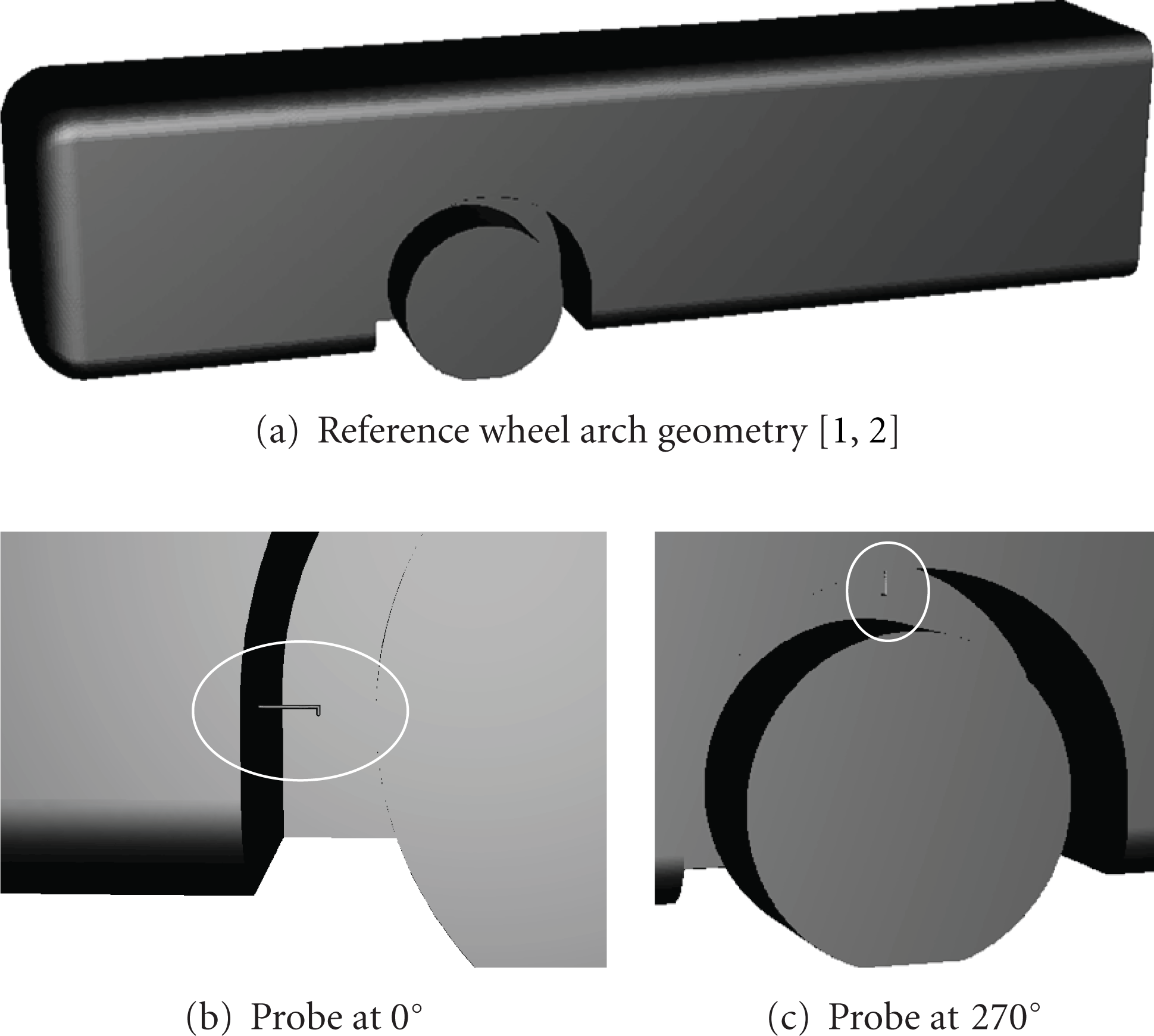
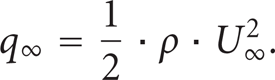
The influence of the presence of the five-hole probe on the flow inside the wheel arch was quantified in terms of the spatial extent of the variation of the pressure and velocity fields caused by it. The flow field values were compared with a reference wheel/wheel arch combination without the probe inserted in it. The vehicle model chosen for this investigation was based on the single-axle front-end model as studied by Fabijanic [2] and later extended by Régert and Lajos [1].

The five-hole probe is inserted inside the wheel arch as shown in Figure 1. The positions around the wheel and its direction of rotation are shown in Figure 2. The location corresponding to 0° is the point facing the direction of travel and 270° is the topmost point of the wheel. All angular positions around the wheel are measured relative to the plane joining the front-facing point and the centre of the wheel, as shown in Figure 2. The probe is laterally aligned with centre line of the wheel. The head of the probe is at the centre of the gap between the wheel and the wheel arch surface. The orientation of the probe head is such that its measuring axis is parallel to the direction of travel.

Figure 1

Five-hole probe located inside automotive wheel arch.

Figure 2

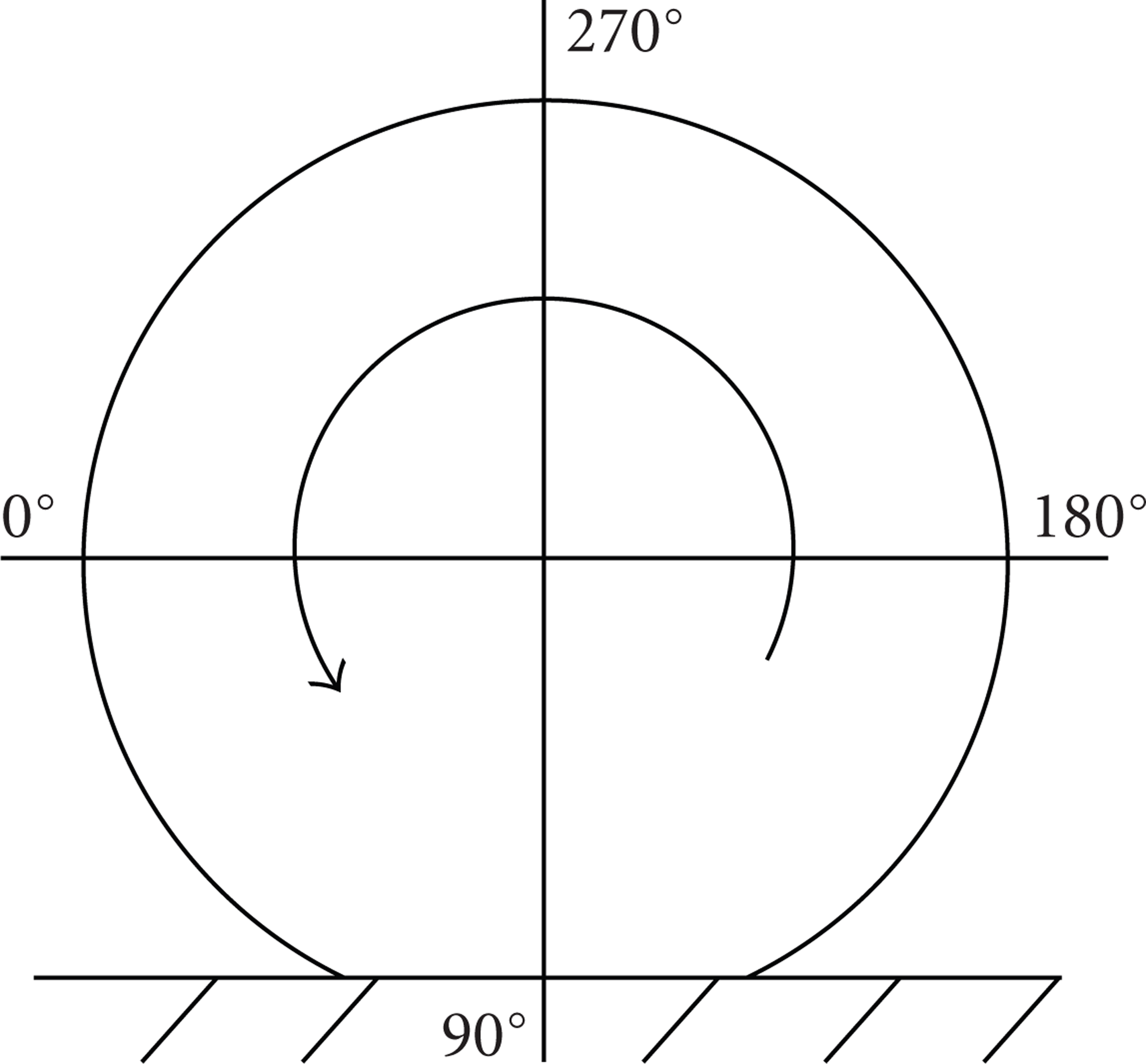
Angular positions and direction of rotation of wheel.

To quantify the influence of the probe on the flow inside the wheel arch the following configurations of wheel arch have been investigated in the present analysis:

• standard Wheel arch—reference configuration (Figure 3(a)),

• wheel arch with probe at the location corresponding to 0° (see circled, Figure 3(b)),

• wheel arch with probe at the location corresponding to 270° (see circled, Figure 3(c)).

CFD geometry of the single-axle vehicle model investigated.

Typical cruising speeds of automobiles range from 40 mph to 70 mph (18 m/s to 31 m/s). The velocity of the generic vehicle in this study has been taken to be 30 m/s (108 km/hour, 67 mph). Reynolds number (Re) based on the width (w = 1.905 m) of the vehicle is 3.91 × 10⁶. The angle of attack of the flow has been maintained at 0° for both configurations investigated.

In Figure 3, the wall at the far inner end of the wheel arch prevents the flow from entering the vehicle body (engine or passenger compartment depending on type of vehicle).

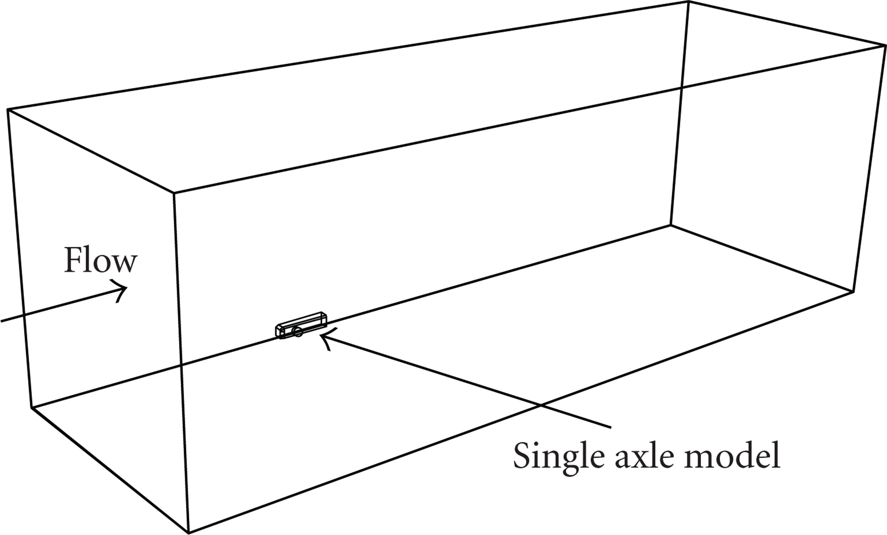
Figure 4 shows details of the simplified model of the single-axle car developed in a computer-aided design (CAD) software package. Only one half of the test geometry was modelled as the geometry and flow conditions were symmetrical about the longitudinal centre plane of the vehicle. The edges of the model had been rounded with a radius of 0.254 m to accurately represent the geometry used by Fabijanic [2] and Régert and Lajos [1]. The rear wheels were not considered in order to study the front wheel and wheel arch combination on the flow field independently. The large distance between the front of the vehicle and the front wheel allows the flow to settle after flowing past the front nose before it reaches the wheel proper.

Figure 4

Dimensions of single-axle vehicle model (m) [1, 2].

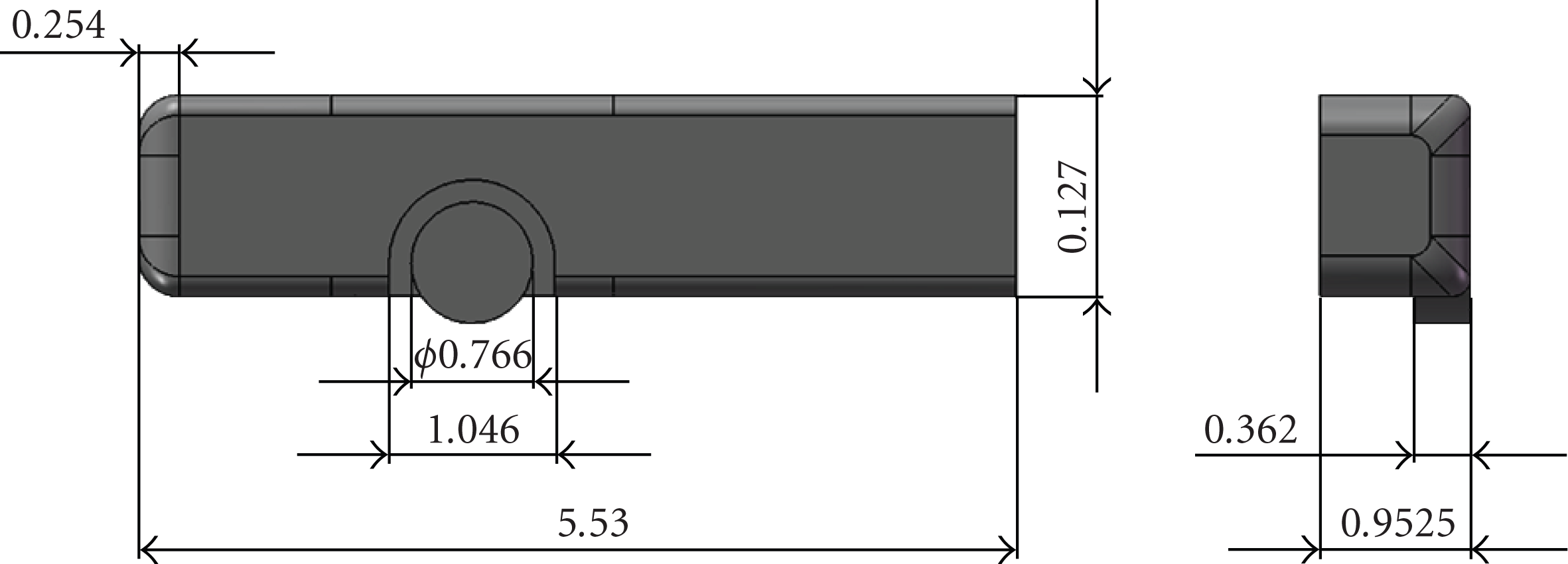
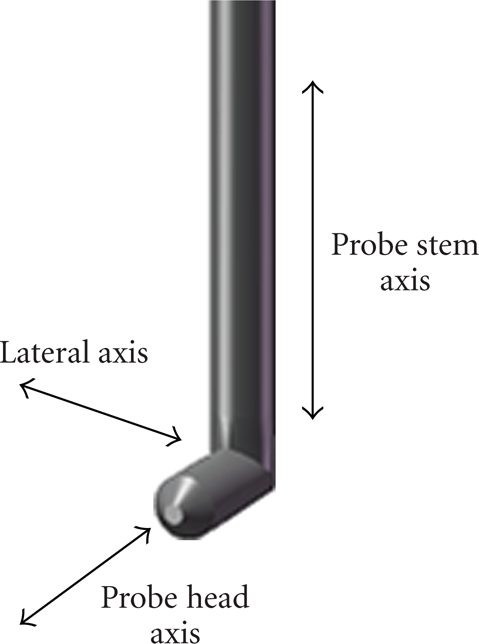
Figure 5 shows the geometry of the five-hole probe used inside the wheel arch. It has a 5 mm stem diameter and an 8.75 mm long head with a 45° conical tip. The axis of the cylindrical stem of the probe is referred to as the probe stem axis. The axis of the cylindrical head of the probe is called the probe head axis. The third axis is the lateral axis which is orthogonal to both the stem and the head axes. The lateral axis passes through the point of intersection of the other two axes. The detailed dimensions are shown in Figure 6. The longitudinal influence of the probe was quantified along the arc (concentric with wheel) tangential to the probe head axis. The vertical influence of the probe was quantified along the probe stem axis. Finally, the lateral influence of the probe was quantified along the lateral axis.

Figure 5

Geometry of five-hole probe.

Figure 6

Dimensions of five-hole probe (mm) [3].

Effect of presence of probe on pressure field has been represented in nondimensional form by using the expression for coefficient of pressure (C_p) as

$C_p=\frac{p-p_{\infty }}{q_{\infty }}.$

(1)

Here p is the local static pressure, p _∞ is the free-stream static pressure, q _∞ is the free-stream dynamic pressure.

If U_∞ is the free-stream velocity, then the dynamic pressure can be represented by the following equation:

$q_{\infty }=\frac{1}{2}·\rho ·U_{\infty }^2.$

(2)

3. Numerical Formulation

The flow field of the single-axle model is simulated using CFD. This includes solving a set of partial differential equations with predefined boundary conditions. The CFD package Fluent 6.3 [23] iteratively solves time-averaged momentum equations along with the continuity equation and appropriate auxiliary equations depending on the type of applications using a control volume formulation. In this study the equations for conservation of mass and momentum have been solved sequentially with two additional transport equations for steady turbulent flow. The SIMPLE pressure-based segregated algorithm was used for pressure-velocity coupling to prevent instability of the solution due to relatively high skewness of mesh elements that was expected around the ground-tyre patch of the wheel. Discretisation of the momentum equations was done by using the Second-Order Upwind scheme to achieve higher accuracy of flow variables at each cell face.

3.1. Mass Conservation

The mass conservation equation given below is valid for both incompressible and compressible flows [23]. The source term S_m is the mass added to the continuous phase from the dispersed second phase (e.g., due to vaporisation of liquid droplets) and any user defined sources:

$\frac{\partial \rho }{\partial t}+\nabla ·\left(\rho \overrightarrow{v}\right)=S_m.$

(3)

3.2. Momentum Conservation

Conservation of momentum in the ith direction in an inertial (nonaccelerating) reference frame is given by the following equation [23]:

$\frac{\partial \left(\rho \overrightarrow{u}\right)}{\partial t}+\nabla \left(\rho \overrightarrow{v}\overrightarrow{v}\right)=-\nabla p+\nabla \left(\stackrel{=}{\tau }\right)+\rho \overrightarrow{g}+\overrightarrow{F}.$

(4)

The stress tensor is given by the following equation [23]:

$\stackrel{=}{\tau }=\mu \left[\left(\nabla \overrightarrow{v}+\nabla {\overrightarrow{v}}^T\right)-\frac{2}{3}\nabla \overrightarrow{v}I\right],$

(5)

where μ is the molecular viscosity, I is the unit tensor, and the second term on the right-hand side is the effect of volume dilation [23].

Fluent uses the finite volume method to solve the time-averaged Navier-Stokes equations and is known for its robustness in simulating many fluid dynamic phenomena. The finite volume method consists of three stages: the formal integration of the governing equations of the fluid flow over all the (finite) control volumes of the solution domain; then discretisation, involving the substitution of a variety of finite-difference-type approximations for the terms in the integrated equation representing flow processes such as convection, diffusion, and sources. This converts the integral equation into a system of algebraic equations, which can then be solved using iterative methods [23]. The first stage of the process, the control volume integration, is the step that distinguishes the finite volume method from other CFD methods. The statements resulting from this step express the conservation of the relevant properties for each finite cell volume [24].

3.3. Computational Domain

The single-axle vehicle model was imported into a three-dimensional flow domain created in Gambit [25]. This flow domain consists of a rectangular cuboid volume which contains the model as shown in Figure 7. The length of the flow domain was 84.67 m, such that the inlet of the flow domain was 3·l upstream of the model (where l is the overall length of the model). The outlet of the domain was 7·l downstream of the model. It was found that 7·l downstream of the model was spatially sufficient to prevent the downstream-imposed constant pressure of 101325 Pa (ambient atmospheric pressure) from having an upstream effect on the pressure field [1]. The width of the flow domain was 27.3325 m (≈5 $·l$ ). This was found sufficient to prevent the interference of the domain wall boundary layer with the flow-field of the model. Similarly, the height of the flow domain was 27.818 m (≈5 $·l$ ). The cross-sectional blockage ratio was found to be 0.16% based on a flow domain cross section area of 760.3 m² and model cross section area of 1.2 m². Since the blockage was extremely low, no corrections were required [26].

Figure 7

Computational domain.

3.4. CFD Mesh Scheme

This resultant flow domain was discretised in Gambit [25] into an unstructured mesh of 12.7 million hybrid tetrahedral cell elements. Mesh quality was controlled such that the space enclosed within the wheel arch and consequently its expected flow-field consisted of smaller elements to increase resolution and ensure reliable results. The resultant mesh is shown in Figure 8 and had a maximum skewness of 0.6 for over 95% of the elements and an aspect ratio between 1 and 2 for over 99% of the elements.

Figure 8

CFD mesh scheme.

The overall flow domain was divided into 6 partitions to distribute the computational load amongst 6 parallel processors. The computational hardware used was a cluster of 6 standard academic desktop computers with dual core processors and 2 GB of physical memory each. Computational time was approximately 9 hours. Due to the large number of mesh elements a mesh independence analysis could not be performed due to severe computational restrictions. However the reliability of the solution was validated against experimental tests and results from earlier research.

3.5. CFD Parameters

Two popular two-equation turbulence models, the realizable k-ε [27] and the SST k-ω [28] models, were considered for this analysis. Both these models are claimed to predict with reasonable accuracy the characteristics of separated flow [1]. It has been found in earlier studies that the realizable k-ε model proved more accurate in calculating flow field parameters for separated flows [1]. Hence the realizable k-ε model was chosen for the analysis. Convergence criteria for the residuals of the transport equations were set to 1 ×10⁻⁴; these criteria were deliberately set too low to ensure that the lowest possible convergence was achieved. Wall roughness for all wall boundaries in the flow domain was ignored and all the wall faces were taken to be smooth.

3.6. Boundaries

The lateral face of the domain ahead of the model was defined as a velocity inlet at a constant velocity of 30 m/s (108 km/hour, 67 mph). The lateral face of the domain behind the model was defined as a pressure outlet at constant atmospheric pressure of 101325 Pa. The bottom face of the flow domain was defined as a moving wall, synchronised with the inlet flow velocity at 30 m/s in the streamwise direction to avoid formation of its own boundary layer which could otherwise modify the flow under the vehicle model. The wheel of the model was defined as moving wall with an angular velocity of 78.329 rad/s about its axle/axis to synchronise it with the relative motion of the vehicle. The vertical wall of the domain forming the longitudinal symmetry plane of the model was specified as a symmetry boundary. All other surfaces of the model, the probe and the domain were specified as stationary walls with no-slip condition.

4. Validation of CFD

To establish the level of accuracy of the CFD results the pressure computed on the pressure taps of the probe tip was compared with experimentally measured values. These validation results are presented in this section. Further verification of the CFD results was carried out; flow field around a model of five-hole probe was computationally simulated in a separate cuboid-shaped flow domain. Flow field interference caused by the probe along the longitudinal axis was taken as the reference parameter. Flow variables computed along this longitudinal axis were compared with earlier research [3].

4.1. Experimental Validation

To ensure that the CFD mesh provided sufficient accuracy, the pressure on five pressure ports on the tip of the probe was computed and compared with those measured experimentally. The validation benchmark experiment was carried out in the low-speed wind tunnel at the University of Huddersfield. The wind tunnel is of open circuit type and has a 1.5 m long test section with a 0.23 m × 0.23 m cross section. Air is provided by an axial blower fan with pneumatically adjustable variable blade pitch. The air speed in the wind tunnel can be varied from 20 m/s to 50 m/s. The walls of the test section were provided with mounting holes and openings for inserting flow measuring devices. The validation was carried out at a flow velocity of 33 m/s and the probe was orientated such that the pitch angle between the probe head axis and the flow was $-{35}^{°}$ and the yaw was $-{40}^{°}$ (please see Figure 10 for definition of pitch and yaw angles). The Reynolds number based on the diameter of the probe (5 mm) was 11292. The blockage was less than 1.5% based on the cross sectional area of the probe (7.7 ×10⁻⁴ m²) and that of the wind tunnel test section (0.05 m²). Hence no blockage correction was required.

The comparison of CFD and experimental results is shown in Figure 9. This plot shows the pressure at the five ports measured experimentally on the horizontal axis. The corresponding pressure values from the benchmark CFD simulation are shown in the vertical axis. The large difference in pressures observed at the five taps is due to the orientation of the probe, the pitch angle being $-{35}^{°}$ and the yaw being $-{40}^{°}$ . This orientation exposes the top and right taps to the oncoming flow and shields the centre, left, and bottom taps from the flow. The pressures computed at the taps were found to be in reasonable correlation with the experimentally measured results (please see Figure 10 for pressure tap designation).

Figure 9

Comparison of CFD experimental values of pressure measured at the five taps (Pa) [3].

Figure 10

Pressure tap designation and orientation of five-hole pressure probe [3].

The CFD code and the mesh scheme could thus be reliably used to analyse the flow field inside the wheel arch. The following section describes the flow field within the wheel arch and a systematic comparison of results obtained with and without the probe inside the wheel arch.

4.2. Comparison with Earlier Work

Further verification of the accuracy of the CFD results was accomplished by numerically simulating the flow field around a five-hole probe in a standard cuboid domain. This was done to accurately reproduce the available reference [3]. The benchmark CFD domain is shown in Figure 11, which is divided into eight smaller volumes to control the mesh quality in the domain.

Figure 11

Validation computational domain [3].

The domain inlet boundary was defined for a free stream air velocity of 33 m/s [3] and the domain outlet was defined at ambient pressure of 101325 Pa. The surface of the probe was specified as a stationary wall. The results of the CFD simulation were compared with the earlier work [3]. Distribution of flow variables was plotted on the longitudinal and lateral planes passing through the stem axis of the probe. In the following description the probe interference effects have been quantified for the benchmark study which would then be compared against previous work.

Figure 12(a) shows contours of x-velocity component in the longitudinal plane passing through the stem axis. This distribution shows that as the flow approaches the probe head, much lower flow velocity is observed immediately upstream of the probe tip. Note that free-stream velocity is along the negative X-direction (X). Although free-stream velocity is 33 m/s, the flow velocity reduces to less than 32 m/s at 1·d upstream of the probe tip (here, d is the diameter of the probe), indicating that the probe presence modifies the velocity field to the magnitude of 3% nearer the probe. On the downstream side the flow reaches near-free-stream velocity in the streamwise (X) direction at 14·d downstream of the probe. Here flow velocity becomes higher than 32 m/s, which is within 5% of the free-stream value.

Contours of flow variables in the longitudinal plane.

Figure 12(b) shows contours of pressure coefficient within the flow domain. It is seen from this distribution that the majority of the domain has a value of C_p in the range of 0 and −0.25. As the flow approaches the probe, the C_p starts to increase until it rises to 1 at the surface where the flow impacts the probe. This occurs on the tip of the probe and the region of the probe stem facing the flow. C_p rises to an average value of 0.25 at 3·d upstream of the tip of the probe (here, d is the diameter of the probe). On the downstream side, it is seen that the value of C_p recovers to its near-free-stream value at a distance of 3·d downstream of the probe stem.

Figure 12(c) shows the contours of y-velocity component (u_y) and clearly establishes the effect of probe in the transverse flow characteristics. It is seen from this distribution that as the flow approaches the tip of the probe, it diverges with positive y-velocity component over the top half of the tip and negative y-velocity component below the bottom half of the tip. Flow is observed to start diverging at a distance of 3·d upstream of the probe tip. This variation of y-velocity component is limited to flow near the probe head region as in the probe stem region the most of the flow divergence takes place in the lateral (Z) direction.

As the flow passes the probe below the probe head it can be seen that, unlike upstream condition, Y component of flow velocity is positive in the downstream side. We would not expect this to happen in absence of the probe. Y-velocity component reduces to less than 1 m/s at a distance of 2·d downstream of the probe head. The magnitude of Y component of velocity is less than 5% of the stream-wise (X) free-stream velocity beyond a distance of 2·d from the probe head indicating almost unidirectional flow.

Upstream values of C_p (deviations are lower in downstream side as compared to x-velocity component deviations) and downstream values of x-velocity component (deviations are less on upstream side as compared to C_p variations) represent the one-dimensional extent of interference caused by the five-hole probe in the streamwise direction. This extends to a distance of 3·d upstream and 13·d downstream of the probe head. The above conclusion correlates well with earlier studies [3] carried out to quantify one-dimensional interference caused by a five-hole probe.

A further verification has been carried out by a comparing gradient of y-velocity component ( $d{u}_y/dx$ ) upstream of the probe with corresponding results from earlier work [3]. This comparison is shown in Figure 13. Results from previous work are plotted along the horizontal axis and those from the current work along the vertical axis. It can be seen from the plot that there is good correlation of the results obtained in current work with those from the earlier work [3].

Figure 13

Comparison of gradient of y-velocity component ( $d{u}_y/dx$ ) with earlier work ( $s^{-1}$ ) [3].

5. Results and Discussion

The flow field parameters (pressure and velocity components) have been investigated for different configurations as described in Section 1. The pressure and velocity fields were plotted along the longitudinal (X-Y) and lateral (Y-Z) planes passing through the probe stem axis in each case with an aim to bring out the effect of probe on flow field change within wheel arch. The following sections describe the distribution of these parameters on these planes.

5.1. Description of Flow in Wheel Arch

The flow within the wheel arch is expected to be largely nonuniform as reported in literature [1, 2]. A review of the literature discussed in Section 1 suggests that three-dimensional flow structures exist in the flow inside the wheel arch. Here the important flow field characteristics within wheel arch are being highlighted with a view to quantify the effects of probe interference on the characteristics.

Figure 14 shows the distribution pressure on the longitudinal plane passing through the centre of the wheel within the wheel arch. This pressure is represented in terms of the nondimensional pressure coefficient (C_p) as defined in (3). It is seen from Figure 14 that C_p is maximum between the angular locations corresponding to 30° and 75°. This is the region on the surface of the wheel where the flow entering the flow field from just below the front body impacts on the tyre surface. Further, it is seen that in the immediate downstream region (after the ground contact region), C_p starts to decrease. The value of C_p is about −0.4 at a location corresponding to 150° beyond which C_p starts to increase until the 180° plane where its value is −0.14. C_p remains fairly constant between locations corresponding to 180° and 270° angles. Further around the wheel surface, C_p decreases to −0.19 between 300° and 330°. Finally, C_p is found to be minimum, −0.4, at the location corresponding to 360°/0°.

Figure 14

Distribution of pressure coefficient (C _p ) on longitudinal plane passing through wheel centre.

The above discussed pressure field can be further clearly seen by distribution of C_p over the surface of the tyre as shown in Figure 15. This figure shows the variation C_p along 11 points on the wheel surface at angular increments of 30°. The discontinuity of this profile between locations corresponding to 60° and 120° in Figure 15 corresponds to the ground/tyre contact patch region which lies outside the computational domain. It is seen from this surface profile of pressure coefficient (C_p) that the coefficient pressure increases in the counter-clockwise direction up to the ground/tyre contact patch region. On the leeward side of the ground contact surface the C_p decreases to a minimum of −0.4 at the angular location corresponding to 150°. As mentioned before between the locations corresponding to 180° and 270°C_p is observed to be fairly constant at −0.14, beyond which it decreases to −0.19 between the locations corresponding to 300° and 330° angles.

Figure 15

Variation of pressure coefficient on wheel surface.

Flow velocity is also affected by the presence of the probe as the latter modifies the velocity field in its vicinity. Figure 16 shows velocity vectors along the longitudinal plane passing through the wheel centre. This Figure shows the general path of the flow along the central plane of the wheel. Flow is seen to impact on the wheel surface between locations corresponding to 45° and about 75°. Separation at the leading edge of the wheel arch causes formation of a recirculation region. This coincides with a low-pressure region, also seen in Figure 14. The counter-clockwise rotation of the wheel causes the reversal of flow near the tyre surface. This can be seen between the locations corresponding to 240° and the 330° where the flow near wheel arch surface is in the clockwise direction and that near the tyre surface is in the counter-clockwise direction.

Figure 16

Vectors of velocity showing the flow pattern with wheel arch.

Detailed investigation of pressure distribution on longitudinal and lateral planes passing through the probe stem axis is required to quantify the effect of the presence of the probe on flow variables along each of the probe axes defined earlier in Section 2 (see Figure 5). Coefficient of pressure (C_p), longitudinal velocity component (u_x), and vertical velocity component (u_y) were investigated in the flow field around the probe within the wheel arch. This was done by comparing distribution of these flow variables along the above two orthogonal planes through the probe stem and the probe head with and without the probe inside the wheel arch. Further investigation of above flow variables was carried out along the arc (concentric with wheel) tangential to the probe head axis. C_p, u_x, and u_y were also investigated along the probe stem axis and the lateral axis of the probe (please see Figure 5 for a description of the probe axes). The locations of these measurement points are shown in Figure 17.

Figure 17

Locations of the measurement points along the primary axes of the probe.

Sections 5.2 and 5.3 describe the influence of probe at locations corresponding to 0° and 270°, respectively, in the wheel/wheel arch gap. A comparison of the above flow variables in the vicinity of the probe with those in the baseline wheel arch (without the probe) at the same location is presented.

5.2. Effect of Probe Inserted at an Angular Location of 0° on Flow Field

The flow field around the probe placed at the location corresponding to 0° in the wheel arch gap was analysed and compared with the reference flow field for the wheel arch without the probe. Please see Figure 2 for a description of angular positions in the wheel arch gap. The following discussion describes the influence of the probe on flow within the wheel arch at this location.

5.2.1. Interference along Probe-Head Axis (Curved)

Coefficient of Pressure (C _p )

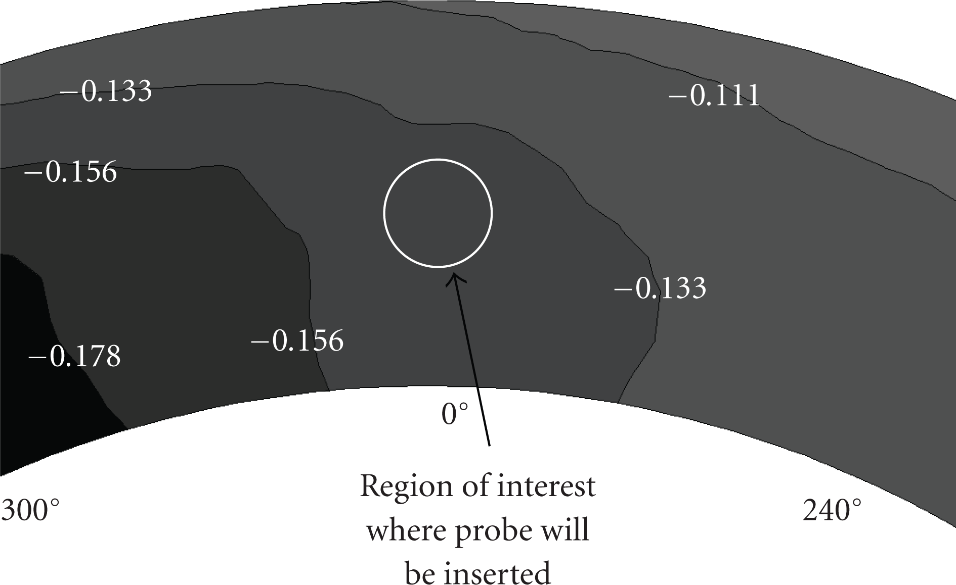
The influence of the probe in front of the probe stem axis was found to be most prominent on the pressure coefficient (C_p). Figure 18 shows contours of pressure coefficient (C_p) on the longitudinal plane passing through the expected probe stem axis at the location corresponding to 0°. This plot covers the region of flow between planes corresponding to 330° and 30° angles. The left extremity of the contour plot depicts the wheel arch inner surface and its right extremity depicts the surface of the wheel. It is seen that C_p is higher than 0.25 near the surface of the wheel near to the location corresponding to 30° as expected [1]. Moreover a region of relatively low-pressure (C_p less than −0.35) is formed immediately downstream of the wheel arch near to the lower end. This can be attributed to the separation of flow that takes place as the air stream enters the wheel arch, as seen in Figure 16. C_p is also seen to decrease upward from the 0° degree location. The location where the five-hole probe is expected to be inserted for later analysis (near-probe region) is shown circled. C_p in this region is found to be −0.275.

Figure 19 shows contours of constant pressure coefficient (C_p) inside the wheel arch on the same longitudinal plane as discussed for Figure 18 with the only difference that in the later case probe is inserted in the flow field. The irregular line passing approximately vertically through the probe head depicts the boundary of the partitions used to distribute the computational load to different processors. It is seen in this figure that the C_p is higher than −0.25 immediately in front of the probe tip. This value of C_p is 5% higher than the C_p found in the near-probe region, also seen earlier in Figure 18. It is clear that this higher value of C_p is a result of the presence of the probe in the flow field. This influence is found to extend up to a distance of 1·d ahead (−Y) of the probe tip (here, d is the diameter of the probe). Similarly, it is seen that C_p is −0.3 immediately behind the probe head. This value of C_p is 5% lower than the C_p found in the near-probe region and extends up to a distance of about 0.5·d in behind (+Y) the probe head.

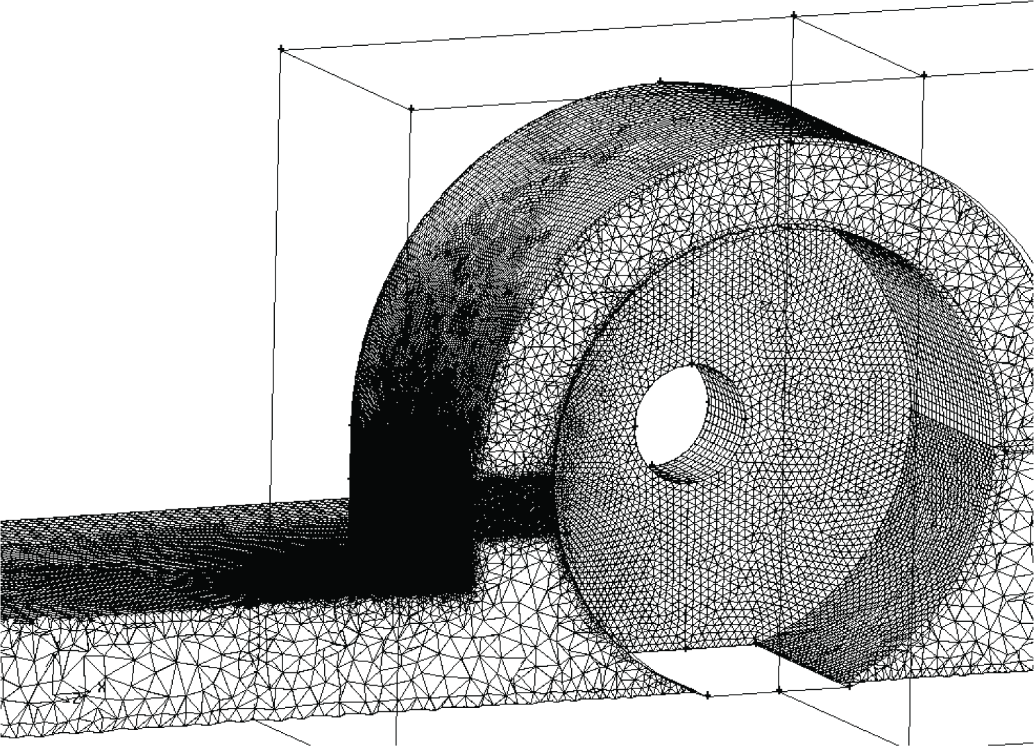
The extent of this interference has been further quantified by plotting a profile of the coefficient of pressure (C_p) in front of the probe tip on the arc (concentric with the wheel) tangential to the probe head axis (please see Figure 17 for location of interrogation points relative to the probe). Figure 20 shows a comparison of C_p immediately in front of the probe tip with that for the baseline configuration at the same location within the wheel arch. The horizontal axis in this plot shows distance ahead of the probe stem axis in multiples of the probe diameter (d). The probe tip is seen to be at a distance of 2.2·d ahead of the stem axis. It is seen that the pressure profile without the probe in the wheel arch is relatively uniform. C_p is found to be −0.25 at the point where the probe tip is expected to be inserted. C_p decreases to about −0.35 at a distance of 10·d ahead of the expected probe stem axis location. When the probe is inserted in the wheel arch, it introduces nonuniformity in this pressure distribution. This nonuniformity extends up to a distance of 3·d ahead of the stem axis (0.8·d ahead of the tip), where the C_p is 15.7% higher than its baseline value (without the probe). This difference decreases to 0.6% at a distance of 4·d ahead of the probe stem axis. Beyond this point it is seen that the influence of probe is negligible on C_p.

Figure 18

Contours of pressure coefficient (C _p ) on longitudinal (X-Y) plane at 0° without the probe.

Figure 19

Contours of pressure coefficient (C _p ) on longitudinal (X-Y) plane with the probe at 0°.

Figure 20

Pressure coefficient (C _p ) profile along arc tangent to probe head axis upstream of the probe at 0°.

Vertical Component of Velocity (u _y )

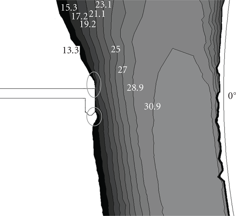
The influence of the probe behind the probe stem axis was found to be most prominent on the vertical velocity component (u _y ). Figure 21 shows contours of vertical component of velocity (u _y ) on the longitudinal plane passing through the expected probe stem axis at the location corresponding to 0°. This plot covers the region of flow between planes corresponding to 330° and 30° angles within the wheel/wheel arch gap. The left extremity of the contour plot depicts the wheel arch inner surface and its right extremity depicts the surface of the wheel. It is seen that near the wheel arch surface u_y is relatively low (between 1 m/s and about 10 m/s) and increases as the distance from the wheel arch surface increases. However near the surface of the wheel high negative velocity is seen. This is due to the rotation of the wheel which in the counter-clockwise (downward, -Y) direction. The location where the five-hole probe is expected to be inserted (near-probe region) is shown circled. The u_y in this region is found to be 14 m/s (upward/clockwise direction).

Figure 22 shows contours of the vertical component of velocity (u_y) inside the wheel arch on the same longitudinal plane as discussed for Figure 21 but with the probe inserted at the location corresponding to 0°. This distribution of u_y shows values of u_y only higher than 13.3 m/s, which is 5% lower than the u_y of 14 m/s found in the near-probe region (see Figure 21). The left boundary of the shaded contour plot represents a constant value of u_y= 13.3 m/s. Although a gradient inu_y exists in the gap (as seen in Figure 21), the probe causes a discontinuity in this gradient immediately in front of the tip and behind the probe head. This is shown circled in Figure 22 and causes the u_y in the immediate vicinity of the probe head to decrease. This is a direct influence of the presence of the probe on the flow field. This influence of the probe extends up to a distance of 1·d ahead and about 2·d behind the probe on the probe head axis (here, d is the diameter of the probe).

Figure 23 shows a comparison of u_y immediately in front of the probe with that for the baseline configuration at the same location within the wheel arch. The horizontal axis in this plot shows distance behind the probe stem axis in multiples of probe diameters (d). The probe stem surface is seen to be at a distance 0.5·d behind the stem axis. At a distance of 3·d behind the stem axis (2.5·d behind the head surface) u_y is found to be 20% higher than its baseline value (without the probe) at the same location. This influence of the probe on the u_y decreases to 3.43% at a distance of 4·d behind the probe stem. Beyond this point it is seen that the influence of probe is negligible on u_y.

Figure 21

Contours of vertical velocity component (u _y ) on longitudinal (X-Y) plane at 0° without the probe.

Figure 22

Contours of vertical velocity (u _y ) on longitudinal (X-Y) plane with the probe at 0°.

Figure 23

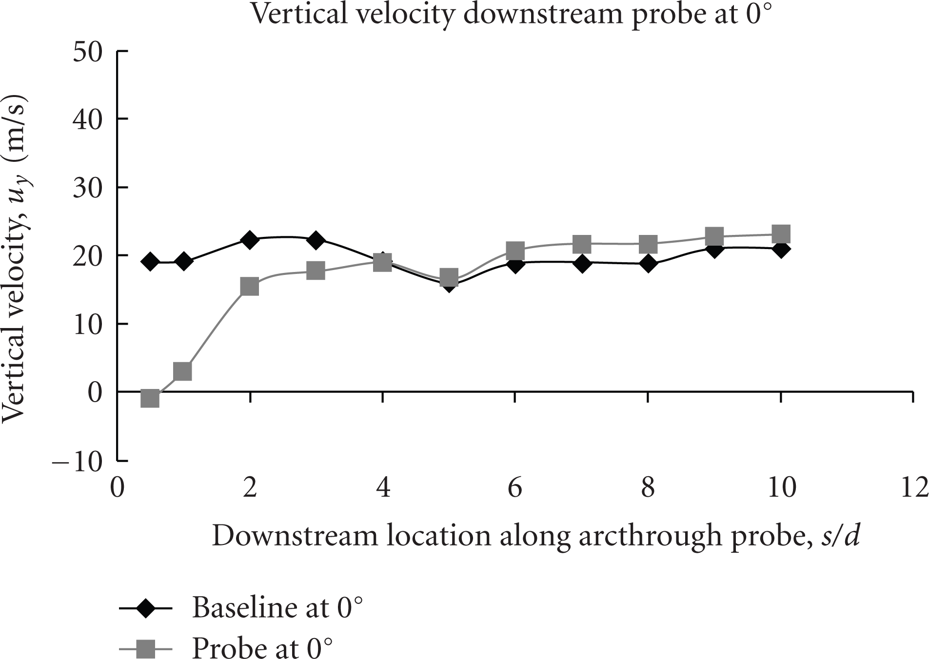
Vertical velocity component (u _y ) profile along arc tangent to probe head axis downstream of the probe at 0°.

5.2.2. Interference along Probe-Stem Axis

Longitudinal Component of Velocity (u _x )

The influence of the probe below the probe head axis was found to be most prominent on the longitudinal velocity component (u_x). Figure 24 shows contours of longitudinal (streamwise) component of velocity (u_x) on the longitudinal plane passing through expected probe stem axis at the location corresponding to 0°. This plot covers the region of flow between planes corresponding to 330° and 30° angles. The left extremity of the contour plot depicts the wheel arch inner surface and its right extremity depicts the surface of the wheel. It is seen that u_x is negative (opposite to streamwise direction) over a large region shown in Figure 24. It is also seen that u_x near the wheel surface is greatly influenced by the rotation of the wheel. u_x is found to be about −9 m/s near the wheel surface between locations corresponding to 330° and 0°, and about +9 m/s near the wheel surface between 0° and 30°. The location where the five-hole probe is expected to be inserted (near-probe region) is shown circled (Figure 24). The u_x in this region is found to be −4.5 m/s.

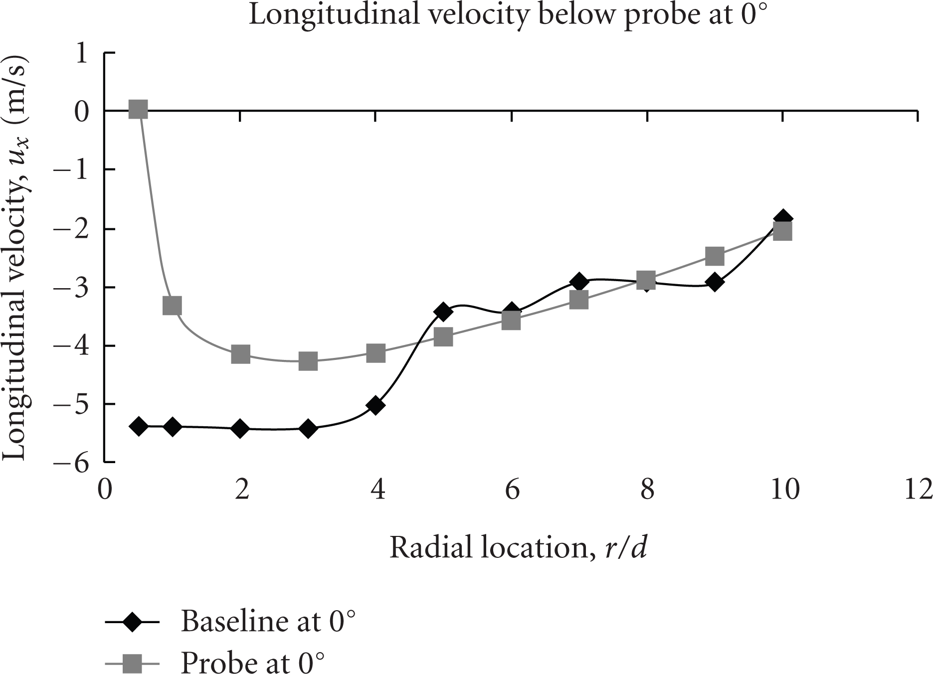
Figure 25 shows contours of the longitudinal component of velocity (u_x) inside the wheel arch on the same longitudinal plane as discussed for Figure 24, but with the probe inserted in the wheel/wheel arch gap at the location corresponding to 0° angle. This plot shows only those values of u_x which are between −5 and −4 m/s. These correspond to −5% and +5%, respectively, of the u_x found in the near-probe region (−4.5 m/s, see Figure 24). The circled areas show the values of u_x beyond this range. The region below the probe head (toward the wheel surface) is seen to have values of u_x higher than −4 m/s. Similarly, the region above the probe tip (toward the wheel arch surface) is seen to have values of u_x lower than −5 m/s. This shows the flow divergence taking place due to the presence of the probe. This region of divergence extends from the probe tip up to a distance of 1·d below the probe head and about 3·d above the probe head (here, d is the diameter of the probe).

Figure 26 shows the profile of the longitudinal velocity component (u_x) along the probe stem axis for a comparison of u_x below the probe with that for the baseline configuration at the same location within the wheel arch. The influence of the presence of the probe extends up to a distance of 5·d below the probe head axis (4.5·d below the surface) where the difference between the magnitude of u_x and its baseline value (without the probe) is found to be 12.3%. This influence decreases to 4.2% at 6·d. Beyond this point it is seen that the influence of probe is negligible on u_x.

Figure 24

Contours of longitudinal velocity component (u _x ) on longitudinal (X-Y) plane at 0° without the probe.

Figure 25

Contours of longitudinal velocity component (u _x ) on longitudinal (X-Y) plane with the probe at 0°.

Figure 26

Longitudinal velocity (u _x ) profile along probe stem axis below the probe at 0°.

5.2.3. Interference along Lateral Axis

Coefficient of Pressure $(C_p)$

The influence of the probe on either side of the probe stem axis was found to be most prominent on the pressure coefficient (C_p). Figure 27 shows contours of pressure coefficient (C_p) inside the wheel arch on a horizontal plane passing through the expected probe stem axis at the location corresponding to 0° (please see Figure 2 for a description of angular positions). The lower extremity of the plot is the wheel surface at the location corresponding to 0° and the upper extremity is the surface of the wheel arch. It is seen that C_p near the inner (left) region is fairly uniform and found to be less about −0.22. Moreover,C_p near the outer (right) region is nonuniform. A region of low-pressure (C_p less than −0.5) is observed immediately downstream of the leading edge of the wheel arch (see top-right, Figure 27). This is associated with the separation of flow occurring at the leading edge of the wheel arch, also seen in the velocity vector plot (Figure 16) in Section 5.1. C_p in the region where the probe head is expected to be inserted (near-probe region, see circled, Figure 27) is about −0.26.

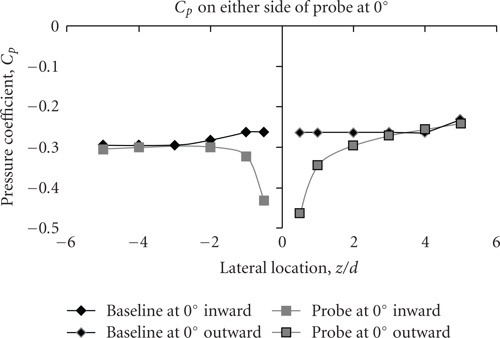
Figure 28 shows contours of pressure coefficient (C_p) on the lateral plane through the probe stem axis with the probe inserted at the location corresponding to 0° in the wheel arch. The lower extremity of the plot is the wheel surface and the upper extremity is the surface of the wheel arch. The C_p in the near-probe region is about −0.26 (also seen in Figure 27). However in the immediate vicinity of the probe head and stem C_p is found to be about −0.3 which is 12% lower than the value in the near-probe region. This is observed up to distance of 1·d on either side of the probe from its surface (here, d is the diameter of the probe).

Further investigation was done to quantify the lateral influence of the probe. Figure 29 shows the profile of the pressure coefficient (C_p) on either side of the probe along its lateral axis. At a distance of 2·d inward from the wheel centre line, C_p is found to be about 6% lower than its baseline value (without the probe). On the outward side, C_p is found to be about 12% lower than its baseline value at a distance of 2·d. Beyond these points on either side the effect of the probe on C_p is found to be less than 4%.

Figure 27

Contours of pressure coefficient (C _p ) inside wheel arch on lateral plane at 0° without the probe.

Figure 28

Contours of pressure coefficient (C _p ) on the lateral plane through probe stem axis with probe at 0°.

Figure 29

Pressure coefficient (C _p ) profile along lateral axis on either side of the probe at 0°.

5.3. Effect of Probe Inserted at an Angular Location of 270° on Flow Field

The flow field around the probe placed at the location corresponding to 270° in the wheel arch gap was analysed and compared with the reference flow field for the wheel arch without the probe. Please see Figure 2 for a description of angular positions in the wheel arch gap. The following discussion describes the influence of the probe on flow within the wheel arch at this location.

5.3.1. Interference along Probe-Head Axis (Curved)

Coefficient of Pressure (C _p )

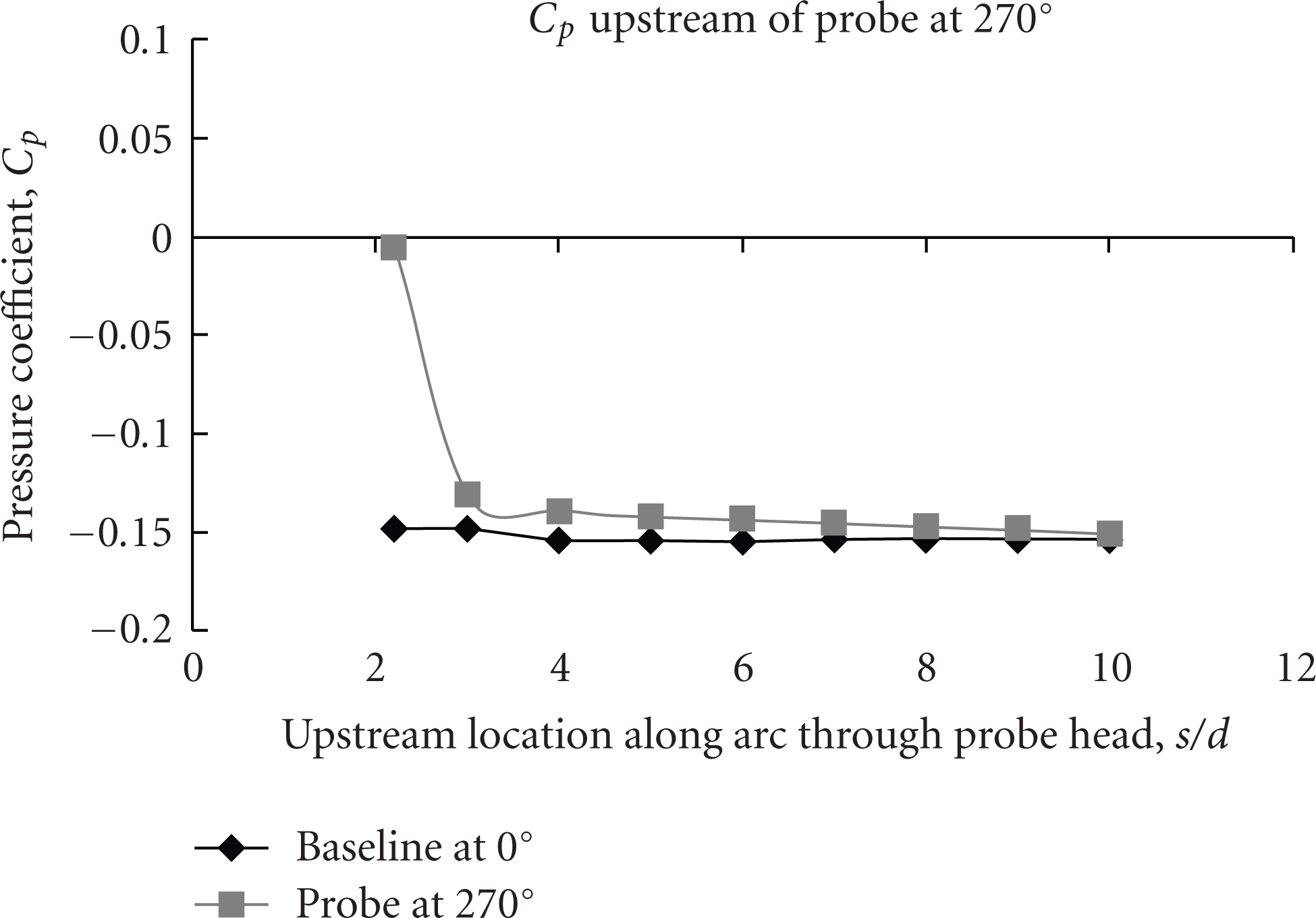
The influence of the probe in front of the probe head was found to be most prominent on the pressure coefficient (C_p). Figure 30 shows contours of pressure coefficient (C_p) inside the wheel arch on a longitudinal passing through the expected probe stem axis at the location corresponding to 270° (please see Figure 2 for a description of angular locations). This plot covers the region of flow between planes corresponding to 330° and 30° angles. The lower curved extremity of the contour plot depicts the wheel surface and it upper extremity depicts the inner surface of the wheel arch. It can be seen from the pressure coefficient distribution that C_p is about −0.18 near the wheel surface at the location corresponding to 300° angle. C_p increases gradually along the streamwise direction (clockwise) up to about −0.12 near the wheel surface at the location corresponding to 240°. It is also seen that C_p increases as the distance along the radial direction increases, which is more prominent between the angular locations corresponding to 270° and 300° angles. The location where the five-hole probe is expected to be inserted for later analysis (near-probe region) is shown circled. C_p in this region was found to be about −0.15.

Figure 31 shows contours of pressure coefficient (C_p) inside the wheel arch on the same longitudinal plane as discussed for Figure 30 but with the probe inserted in the wheel/wheel arch gap at the location corresponding to 270° angle. High C_p is expected on the front side of the probe stem and on the tip where the flow impacts these regions [3]. The C_p in the near-probe region is about −0.15. The influence of the probe tip is identified by the higher C_p in front of the probe tip. This value of C_p was found to be −0.14 which is about 7% higher than the C_p of the near-probe region. This influence of the probe extends up to a distance of about 2·d ahead of the probe tip. Similarly C_p immediately behind the probe head was found to be much lower than its reference baseline value at −0.156 and extends up to a distance of about 1·dbehind the probe stem (here, d is the diameter of the probe).

Figure 32 shows a profile of the coefficient of pressure (C_p) on the arc (concentric with the wheel) tangential through the probe head axis. The horizontal axis in this plot shows distance ahead of the probe stem axis in multiples of the probe diameter (d). The probe tip is seen to be at a distance of 2.2·d ahead of the stem axis. When the probe is inserted in the wheel arch, it introduces nonuniformity in this pressure distribution. This nonuniformity extends up to a distance of 6·d ahead of the stem axis (3.8·d ahead of the tip), where the C_p is 7.1% higher than its baseline value. This difference decreases to about 5% at a distance of 7·d ahead of the probe stem axis. Beyond this point it is seen that the influence of probe is negligible on C_p.

Similarly, to quantify the downstream interference caused by the probe, Figure 33 shows a comparison of C_p behind the probe with that for the baseline configuration at the same location within the wheel/wheel arch gap. The horizontal axis in this plot shows distance behind the probe stem axis in multiples of the probe diameter (d). When the probe is inserted in the wheel arch, it influences the C_p immediately behind the probe head, which is found to be much lower than the corresponding baseline values (without the probe). This influence extends up to a distance of 1·d behind the stem axis (0.5·d behind the stem surface), where the C_p is 6.5% lower than its baseline value. This difference decreases to about 0.5% at a distance of 2·d behind the probe stem axis. Beyond this point it is seen that the influence of probe is negligible on C_p.

Figure 30

Contours of pressure coefficient (C _p ) on longitudinal (X-Y) plane at 270° without the probe.

Figure 31

Contours of pressure coefficient (C _p ) inside wheel arch on longitudinal (X-Y) plane with the probe at 270°.

Figure 32

Pressure coefficient (C _p ) profile along arc tangent to probe head axis upstream of the probe at 270°.

Figure 33

Pressure coefficient (C _p ) profile along arc tangent to probe head axis downstream of the probe at 270°.

5.3.2. Interference along Probe-Stem Axis

Longitudinal Component of Velocity (u _x )

Figure 34 shows contours of longitudinal component velocity (u_x) inside the wheel arch on a longitudinal plane where the probe is to be inserted at the location corresponding to 270°. The shaded regions along the middle of the gap show flow velocities between −1 m/s (counter-clockwise) and 10 m/s (clockwise). u_x is seen to be predominantly positive near the wheel arch surface where it is greater than 10 m/s (shown by the white space above the shaded contour region). u_x is found to be negative for the region near the wheel surface, where its magnitude is greater than 1 m/s (shown by the white space below the shaded contour region). This opposite flow velocity can be attributed to the rotation of the wheel and its associated boundary layer. The u_x in the region where the location was of the probe head is expected (near-probe region, see circled, Figure 34) is 4.5 m/s.

Figure 35 shows contours of longitudinal velocity component (u_x) inside the wheel arch on the same longitudinal plane as discussed for Figure 34, but with the probe inserted in the wheel/wheel arch gap at the location corresponding to 270°. Although the u_x found in the near-probe region was found to be about 4.5 m/s (see Figure 34), the presence of the probe is seen to influence the u_x in the region below the probe head (toward the wheel surface). Here u_x is found to be lower than 3.2 m/s. This region of low u_x is seen to merge with the existing low-u_x region in the flow below the probe. Hence, the extent of this lower velocity caused by the probe cannot be quantified clearly. Investigation of the velocity profile along the probe stem axis will further assist in clearly quantifying the influence of the probe in this direction.

Figure 36 shows a profile of the longitudinal velocity component (u_x). The insertion of the probe in the flow field at this location (270°) influences the longitudinal velocity component in its vicinity. This influence is seen to extend up to a distance of 7·d below the probe head axis (0.5·d below the surface), where the difference between u_x and its corresponding baseline value (without the probe) is found to be 74%. Beyond this point it is seen that the influence of probe is negligible on u_x.

Figure 34

Contours of longitudinal velocity component (u _x ) inside wheel arch on longitudinal (X-Y) plane at 270° without the probe.

Figure 35

Contours of longitudinal velocity component (u _x ) inside wheel arch on longitudinal (X-Y) plane with the probe at 270°.

Figure 36

Longitudinal velocity component (u _x ) profile along probe stem axis below the probe at 270°.

5.3.3. Interference along Lateral Axis

Coefficient of Pressure (C _p )

The influence of the probe on either side of the probe stem axis was found to be most prominent on the pressure coefficient (C_p). Figure 37 shows contours of pressure coefficient (C_p) on a lateral plane passing through the expected probe stem axis at the location corresponding to 270° inside the wheel arch. The lower extremity of the plot is the wheel surface and the upper extremity is the surface of the wheel arch. It is seen that C_p near the wheel surface is about −0.14. C_p increases fairly uniformly as the radial distance from the wheel surface increases until it becomes approximately −0.1 near the surface of the wheel arch. The C_p in the region around where the probe head is expected to be inserted (near-probe region, see circled, Figure 37) is about −0.14.

Figure 38 shows contours of pressure coefficient (C_p) on the lateral plane passing through the probe stem axis when the probe is inserted at the location corresponding to 270°. The lower extremity of the plot is the wheel surface and the upper extremity is the surface of the wheel arch. It is seen that the distribution of C_p in this region is largely similar to that found for the baseline wheel arch (without the probe). The C_p in the near-probe region is about −0.14. However in the immediate vicinity of the probe head and stem C_p lower than −0.16 is observed up to a distance of 1·d on either side of the probe (here, d is the diameter of the probe). This influence of the probe on C_p is more pronounced near the wheel arch surface from where the probe is inserted into the wheel arch gap. Here, C_p of less than −0.1 is observed up to a distance of about 3·d on either side of the probe.

Further investigation of the profile of the pressure coefficient (C_p) on either side of the probe on its lateral axis was done to quantify the lateral influence of the probe. Figure 39 shows a comparison of C_p on either side of the probe with that for the baseline configuration (without the wheel arch) at the same location within the wheel arch. It is seen that C_p is nearly constant at about −0.15 without the probe in this region. The introduction of the probe at this location shows lower C_p in its immediate vicinity. On the inward surface of the probe head C_p is found to be about 4% lower than its baseline value. Moreover, C_p is seen to be about 7% higher than its baseline value at a distance of 2·d inward from the probe stem. On the outward side, C_p is found to be about 12% lower than its baseline value at a distance of 1·d from the probe stem axis. Beyond these points on either side the effect of the probe on C_p is found to be less than 4%.

Figure 37

Contours of pressure coefficient (C _p ) inside wheel arch on lateral plane through expected probe stem axis at 270° without the probe.

Figure 38

Contours of pressure coefficient (C _p ) on the lateral plane through probe stem axis at 270°.

Figure 39

Pressure coefficient (C _p ) profile along lateral axis on either side of the probe at 270°.

5.4. Overall Influence of the Probe

The description of influence of the probe in each direction discussed in Sections 5.2 and 5.3 suggests that the interference in each direction is quantified by considering the flow variable that is most influenced by the probe in that direction. Only the variables most affected by the presence of the probe have been presented for brevity. Table 1 shows a brief outline of the interference caused by the probe at the two locations discussed in Sections 5.2 and 5.3. It is seen that there is no direct relation between the influence of the probe at the locations corresponding to 0° and 270°. This can be associated with the nonuniformity of the flow within the wheel arch. Further analysis is required to develop a generic model for the three-dimensional interference caused by such an intrusive flow measuring device. However the extent of interference caused by the probe along its axes has been clearly identified.

Table 1:

Outline of probe influence at investigated locations (d = probe diameter).

Probe location	Ahead of probe	Behind probe	Below probe head	Inward	Outward
0°	3·d	3·d	5·d	2·d	2·d
270°	6·d	1·d	7·d	2·d	1·d

The influence of the probe along the probe head axis was seen to be up to a distance of 3·d ahead of the probe stem axis for the probe at the location corresponding to 0° and up to 6·d ahead for 270°. This influence was found to extend up to a distance of 3·d behind the probe stem axis for the probe at the location corresponding to 0° and 1·d behind for 270°. The interference below the probe head (radially toward the wheel) was found to be up to a distance of 5·d below the probe head axis for the probe at the location corresponding to 0° and up to 7·d below the probe head for 270°. Finally the influence of the probe in the lateral direction (perpendicular to both probe head axis and probe stem axis) was found to be about 2·d on either side of the probe stem. This three-dimensional extent of interference of the probe discussed represents the influence of the probe on the flow field inside the wheel/wheel arch.

The extent of interference in each direction can be associated with the corresponding radius of an imaginary ellipsoid. This can be used to form a three-dimensional region of influence as shown in Figure 40.

Figure 40

Three-dimensional ellipsoid of interference caused by five-hole probe.

Hence the major (along the probe head axis) and minor (along the lateral probe axis) equatorial radii of the imaginary ellipsoid of interference caused by the probe were found to be of lengths 6·d and 2·d, respectively. The polar (along the probe stem axis) radius of this ellipsoid was found to be of length 7·d (here, d is the diameter of the probe). During the placement of probes, the minimum distance between two probes must not be less than twice the extent of interference of a single probe along any direction.

6. Conclusion

Flow field analysis inside the wheel arch of a single-axle vehicle was carried out using validated CFD simulations at nominal cruising velocity. Velocity and pressure distribution along orthogonal planes passing through the stem axis of a five-hole pressure probe at different locations inside the wheel arch were investigated. This was done with and without the probe inside the wheel/wheel arch gap to quantify the extent of interference caused by the probe on the flow field. It was found that the interference caused by the probe along the probe head axis was found to extend up to a distance of 6·d ahead of the probe head and 3·d behind it. Moreover, this interference extends up to a distance of 7·d below the probe head (along the probe stem axis) and up to 2·d on either side of the probe head. These extents of interference define a three-dimensional ellipsoid of interference around each probe in the flow. This can be used to optimally place the probes in small regions such as the wheel arch investigated herein. To ensure high accuracy of flow measurements, the minimum distance between two probes must be such that ellipsoids of interference of adjacent probes must not intersect at any point in the region being investigated. Hence the lateral distance between two probes must not be less than 4·d. Similarly the longitudinal distance between two probe must not be less than 12·d. Finally the vertical distance between two probes must not be less than 14·d.

The present study has quantified the three-dimensional extent of interference caused by the probe inside the wheel arch at nominal vehicle velocity. These results can be used to optimally arrange an array of such instruments inside the automotive wheel arches to accurately map the flow with minimal errors due to flow-field interaction between nearby probes. The optimal placement of pressure probes inside the wheel arch will allow recording of accurate transient flow parameters which would otherwise be affected by probe interference. This will immensely help in the investigation of transient pressure and velocity measurements in the flow field around automotive disc brakes, wheels, as well as inside wheel arches. Further, a better insight can be gained into the influence of such transient flow on the overall forces and moments on automobiles and hence help in the investigation of ground vehicle stability under transient conditions like cross winds and gusts.