Sage Journals: Discover world-class research

Abstract

The kinematic and dynamic analyses of a PKM mesomanipulator are addressed in this paper: the proposed robot architecture allows only pure translations for the mobile platform, while the presence of flexure hinges introduces compliance into the structure. The analytical solutions to direct and inverse kinematic problems are evaluated after a brief introduction of the basic adopted nomenclature, the manipulator workspace and the robot singularity configurations are then described, and the analytical solution to the inverse dynamic problem is presented. Thereafter, an overview on some of the simulations results obtained through a software implementation of the described algorithms is addressed, and the most salient aspects of this topic are summarized in the final conclusions.

1. Introduction

Parallel manipulators assure high accuracy and high accelerations but a limited workspace [1]. The mesomanipulator herein concerned, as shown in Figure 1, results characterized by a parallel architecture, and by the presence of flexural hinges joints between the links, that introduce compliances into the structure [2].

Figure 1

The PKM mesomanipulator.

A peculiar characteristic of the robot is the possibility to generate the final configuration from an original planar structure, through opportune plastic deformations in the proper flexure hinges.

In this paper, the kinematic analysis of the mesomanipulator will be addressed: forward and inverse analytical solutions will be presented, then the singular configurations and the robot workspace will be taken into account; once the dynamic analysis is described, the main elements of the mesomanipulator analysis will be finally presented.

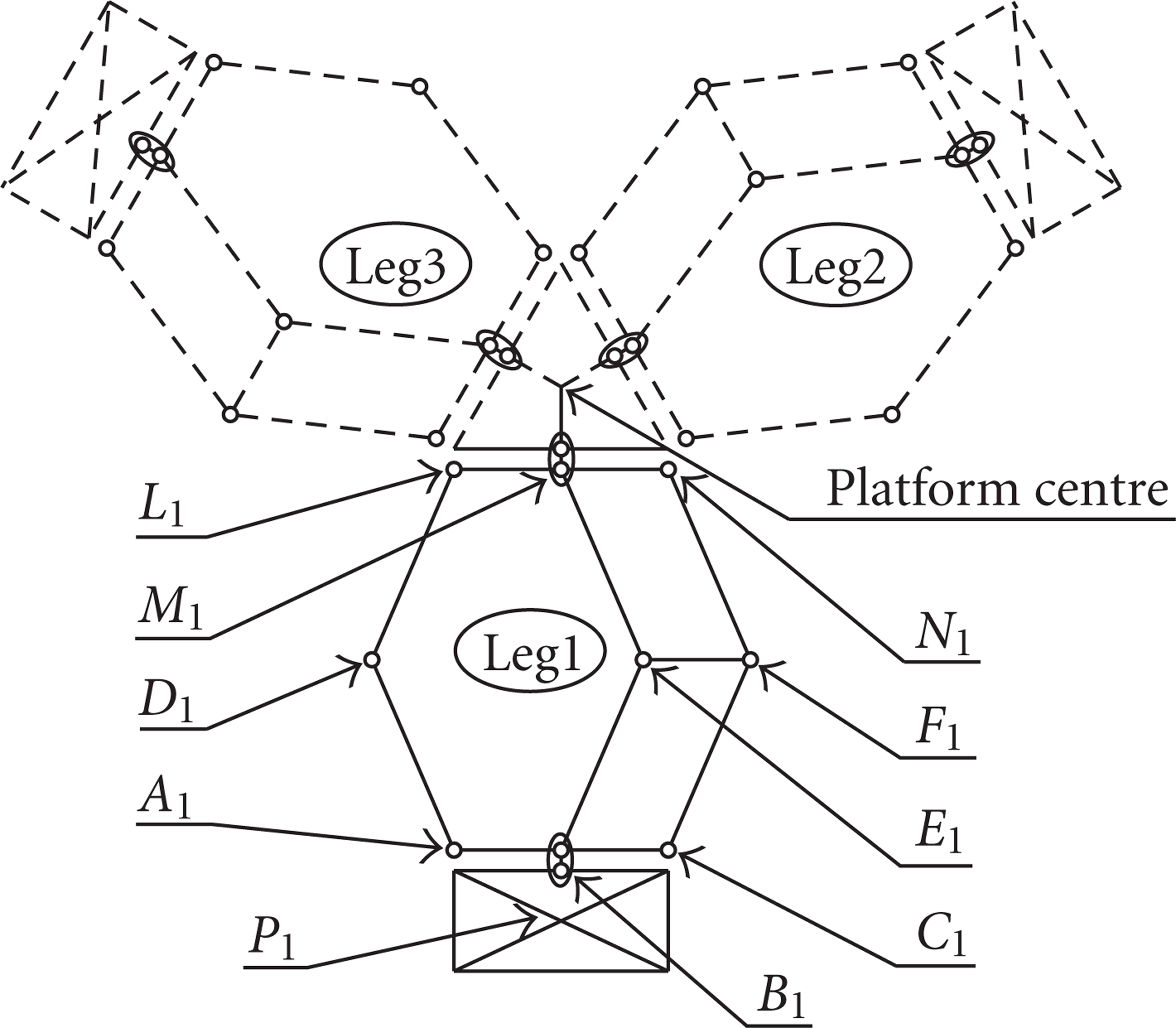
The robot frame presents a strong symmetry, involving three kinematic chains (in the following leg 1, leg 2, and leg 3, as presented in the model scheme of Figure 2) that link each fixed element, called feet (P_iwith $i = 1,2, 3$ in agreement with the respective leg number), with the central mobile platform [3].

Figure 2

The manipulator planar structure: basic adopted nomenclature.

As shown in Figure 2, two four-bar mechanisms in cascade can be identified in every leg, and these are determined by the so-called B_i, C_i, E_i, F_i and E_i, F_i, M_i, N_i points, while, on the other hand, an isostatic triangle can be defined by the A_i, D_i,and L_i points of every leg: the first structure allows the platform just pure translation movements [4], while the presence of the isostatic element nothing adds to the kinematic structure functionality and can therefore be neglected in a functional analysis [5].

Particular attention is paid to the evaluation of the structure degrees of freedom (dof): the model presented in Figure 3 illustrates the basic hypotheses that lead to assume 132 dof and 129 doc (degrees of constraint), in agreement with the total 3 dof of the functional structure [6]. As a matter of fact, the structural scheme in Figure 2 introduces fictitious functional multiple joints, due to the geometrical simplified connections adopted between the links and the mobile platform or between each leg and its foot; for this reason the functional scheme in Figure 3 does not prevent from the assumption of multiple and coinciding flexural joints.

Figure 3

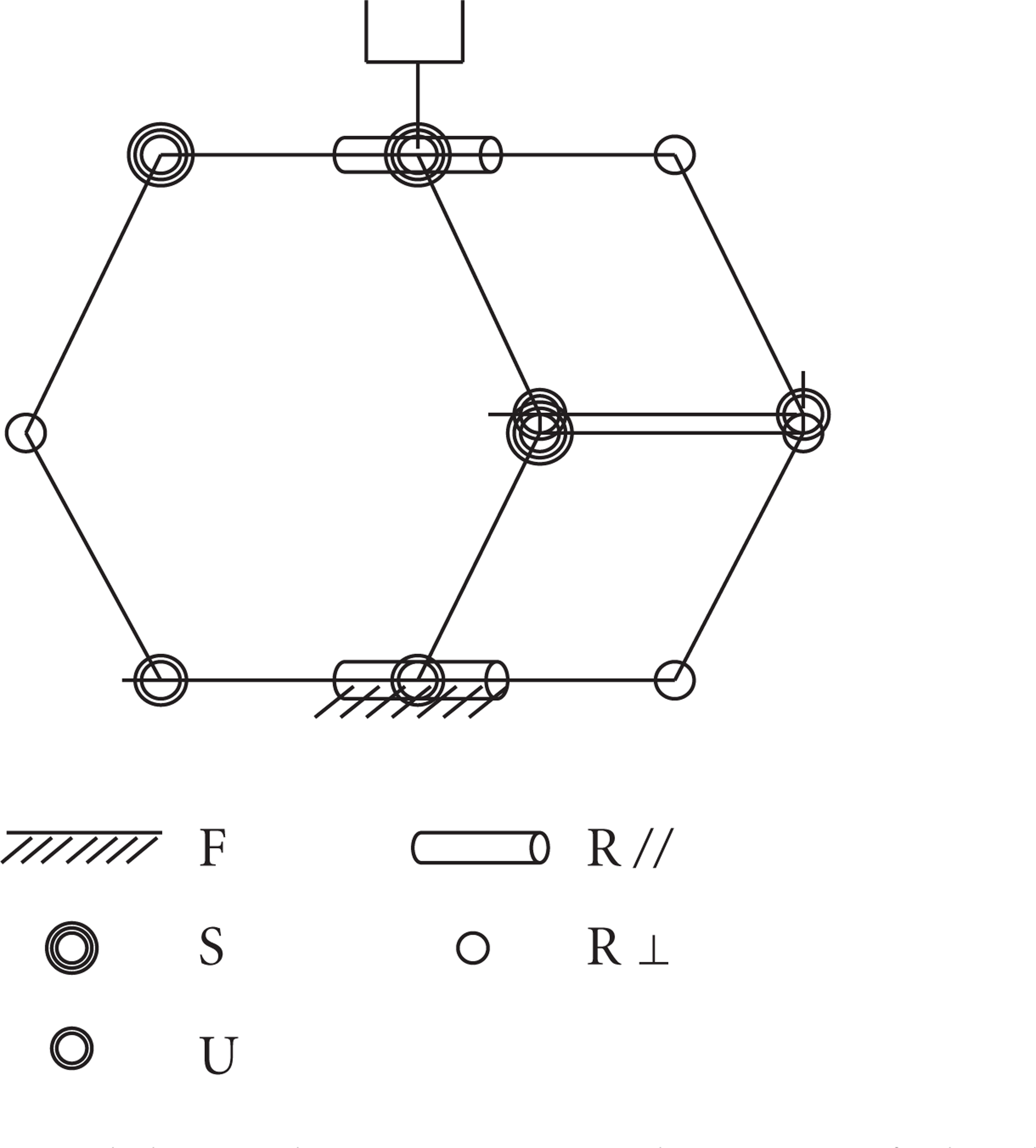
Functional leg scheme. From the top of the legend: F the frame, S the Spherical joints, U the Universal joints, and R the Rotoidal ones, with the rotational axis parallel or orthogonal respectively to the sheet plain.

2. Kinematic Analysis

The robot symmetry simplifies the kinematic problem allowing the identification of an analytical solution [7]: once defined the foot position into an absolute and fixed reference system, the position of the mobile platform centre, indicated by the column vector S as presented into the relation (1), results univocally identified by a tern of variable distances, whose expressions result strictly related to the actuators positioning:

S = {[\begin{bmatrix} x_{S} & y_{S} & z_{S} \end{bmatrix}]}^{'} .

(1)

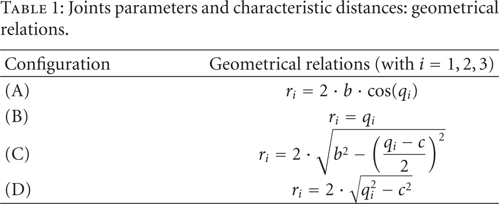
In particular, four different configurations have been identified for the three required actuators, as Figure 4 shows; all of them are referable to the first one presented, through the simple geometrical transformations described in Table 1, where Q indicates the column vector (2) collecting the joints parameters and R is the column vector (3) of the $B_{i} M_{i}$ distances (once again $i = 1,2, 3$ in agreement with the leg number), while b and c identify, respectively, the links and the rocker arms lengths:

Table 1:

Joints parameters and characteristic distances: geometrical relations.

Configuration	Geometrical relations (with $i = 1,2, 3$ )

(A)	$r_{i} = 2 \cdot b \cdot \cos (q_{i})$
(B)	$r_{i} = q_{i}$
(C)	$r_{i} = 2 \cdot \sqrt{b^{2} - {(\frac{q_{i} - c}{2})}^{2}}$
(D)	$r_{i} = 2 \cdot \sqrt{q_{i}^{2} - c^{2}}$

Figure 4

Manipulator actuation: the four identified configurations.

\begin{align} Q & = {[\begin{bmatrix} q_{1} & q_{2} & q_{3} \end{bmatrix}]}^{'}, \end{align}

(2)

\begin{align} R & = {[\begin{bmatrix} r_{1} & r_{2} & r_{3} \end{bmatrix}]}^{'} \end{align} .

(3)

Observing that the geometrical constant values of the foot (the a lengths) and of the platform (the d lengths) do not influence the platform centre position, the equivalent and simplified model shown in Figure 5 can be considered [8]: the general kinematic relation (4) for the positions becomes therefore the system (5) of three equations, each of whom representing a sphere, with r_i radius (function of q_i) and centre in the i -feet in the simplified equivalent kinematic model, where $i = 1,2, 3$ :

Figure 5

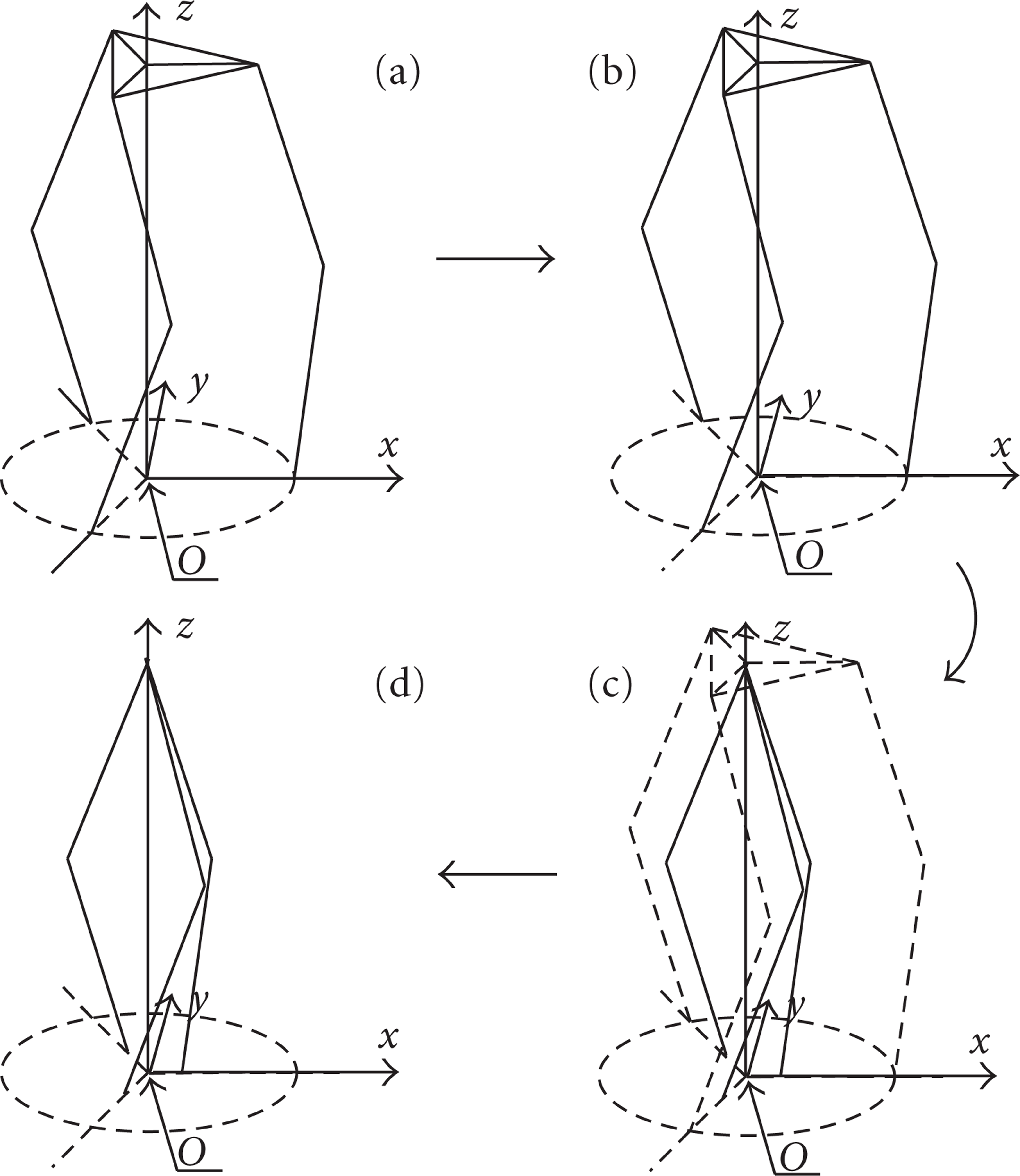
Consecutive geometrical simplifications allow to reach the simplified equivalent kinematic model (d) starting from the original configuration (a); in (b) the first translation removes the a lengths, while in (c) the second translation removes the d lengths.

\begin{gathered} S = F (Q), \end{gathered}

(4)

\begin{gathered} {(x_{S} - x_{i})}^{2} + {(y_{S} - y_{i})}^{2} + {(z_{S} - z_{i})}^{2} = r_{i}^{2} . \end{gathered}

(5)

For the sake of simplicity, the (B) configuration will be taken into account in the current analysis, even if the presented procedure could be adopted to analyze also the other configurations.

Under these hypotheses, the inverse kinematics can be easily reduced to the system (6), generating two solution vectors: the negative one has been neglected as unreachable for physical considerations:

q_{i}^{2} = {(x_{S} - x_{i})}^{2} + {(y_{S} - y_{i})}^{2} + {(z_{S} - z_{i})}^{2} .

(6)

Also the direct kinematics can be easily evaluated, as the system (7) describes; once again, the negative solution has been discarded:

\begin{matrix} x_{S} & = \frac{q_{3}^{2} + q_{2}^{2} - 2 \cdot q_{1}^{2} - 2 \cdot x_{2}^{2} - 2 \cdot y_{2}^{2} + 2 \cdot x_{1}^{2}}{4 \cdot x_{1} - x_{2}}, \\ y_{S} & = \frac{q_{3}^{2} - q_{2}^{2}}{4 \cdot y_{2}}, \\ z_{S} & = \pm \sqrt{q_{1}^{2} - y_{S}^{2} - {(x_{S} - x_{1})}^{2}} . \end{matrix}

(7)

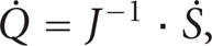
The direct kinematic analysis for velocity $\dot{S}$ and acceleration $\ddot{S}$ requires the introduction of the Jacobian matrix J and its time derivate [9].

The velocity and acceleration inverse kinematics consists in the solution of the matrix relations (8) and (9), where the mathematical constraints to the inversion of the Jacobian matrix identify the robot singularities, as presented in the followings:

\begin{align} \dot{Q} & = J^{- 1} \cdot \dot{S} \end{align},

(8)

\begin{align} \ddot{Q} & = J^{- 1} \cdot \ddot{S} + {\dot{J}}^{- 1} \cdot \dot{S} \end{align} .

(9)

3. Singularity Configurations and Robot Workspace

As previously introduced, not all the ideally reachable positions can be supported by the analytical algorithm chosen to solve the kinematics: in fact, the adopted actuators configuration directly influence the Jacobian matrix definition.

Considering, for instance, the (B) configuration, the Jacobian determinant becomes equal to zero when at least one of the relations (10), (11), or (12) is verified, that is, when the platform centre belongs to the plain identified by the three feet:

\begin{align} q_{1} & = {0}, \end{align}

(10)

\begin{align} q_{2} & = {0}, \end{align}

(11)

\begin{align} q_{3} & = {0} \end{align} .

(12)

Changing the actuator configuration, the Jacobian matrix assumes different singularity conditions, as Table 2 presents.

Table 2:

Robot singularities.

Conf.	Singularity Conditions

(A)	$q_{1} = {0, π / 2}$ ; $q_{2} = {0, π / 2}$ ; $q_{3} = {0, π / 2};$
(C)	$q_{1} = {c}$ ; $q_{2} = {c}$ ; $q_{3} = {c};$
(D)	$q_{1} = {0}$ ; $q_{2} = {0}$ ; $q_{3} = {0};$

Two observations are worth to be underlined, related to the actuators configuration.

First of all, it is to note how the (B) configuration, here chosen as the basic one, not only represents, from a computational viewpoint, the easiest adoptable solution but also avoids physically reachable singularities; then, choosing another actuators configuration the number of singularities or their functional relevance could increase, as the (A) and (C) demonstrate, respectively.

All the other positions, physically reachable by the platform centre, contribute to define the robot workspace (WS), qualitatively shown in Figure 6 [10].

The robot workspace: black: the feet of the first leg; red the feet of the second and green of the third one.

In particular, the planar view, more than the others, allows to appreciate how the WS represents the intersection of the three spheres, each of them centered in one of the foot.

This ideal WS should actually be reduced, because of the flexure hinges adopted as joints. For instance, under the hypothesis of the simplified hinge model shown in Figure 7, and the use of homogeneous PTFE material (Table 3 for the characteristics), the maximum deflection angle can be easily evaluated as expressed by the relation (13); if considering the maximum radius of curvature that the beam can bear before yielding, under a pure bending moment, it can be determined through the relation (14):

Table 3:

Adopted parameters value for the PTFE-simplified hinge model.

Parameters	Value

E (Young modulus)	500·103 [MPa]
σ _Yield	50 [MPa]
h	0.2 [mm]
L	3 [mm]

Figure 7

Simplified hinge model.

\begin{align} Θ_{Yield} & = \frac{L}{ρ_{Yield}}, \end{align}

(13)

\begin{align} \frac{1}{ρ_{Yield}} & = \frac{2 \cdot σ_{Yield}}{h \cdot E} . \end{align}

(14)

Once defined the generic deflection angle Θ_n ( $n = 1, \dots N$ , with N the total hinges number) that the nth hinge assumes at the generic instant t and forcing simultaneously all the hinges to verify the reachability condition (15), the reduced WS qualitatively can be identified as shown in Figure 8:

The robot reduced workspace [m]: black: the feet of the first leg; red the feet of the second and green of the third one.

Θ_{n} \leq Θ_{Yield} .

(15)

4. Dynamic Analysis

Further elements need to be introduced to analyze the robot dynamic behavior: a column vector F_s of all the generalized forces (forces and torques) applied to the platform centre, the column vector F_q of the generalized forces applied to the actuated joints, and the diagonal mass matrix ℳ containing the mass property of all the “interesting” points, that is, the generalized forces act along those coordinates (joints and platform centre for this treatment) [11].

For this reason, the S and Q vectors need to be rewritten as S_d andQ_d, accordingly to the identification of the new interesting coordinates, and also J will change consequently its form.

The further step requires to distinguish, into the definition of F_s, between externally imposed forces and inertial ones, as the relations (16) and (17) present:

\begin{align} F_{s} & = F_{s e} + F_{s i}, \end{align}

(16)

\begin{align} F_{s i} & = - ℳ {\ddot{S}}_{d} . \end{align}

(17)

All these elements are combined into the expression (18), representing the dynamic problem in the classical formulation [12], with $\bar{ℳ}$ , 풱, and 풢 defined as the relations (19),(20), and (21) describe:

\begin{gathered} \bar{ℳ} (Q_{d}) {\ddot{Q}}_{d} + ν (Q_{d}, {\dot{Q}}_{d}) + 풢 (Q_{d}, F) = 0, \end{gathered}

(18)

\begin{matrix} \bar{ℳ} (Q_{d}) = J^{T} ℳ J, \end{matrix}

(19)

\begin{matrix} ν (Q_{d}, {\dot{Q}}_{d}) = (J^{T} ℳ \dot{J}) {\dot{Q}}_{d}, \end{matrix}

(20)

\begin{gathered} 풢 (Q_{d}, F) = - (J^{T} F_{s e} + F_{q}) . \end{gathered}

(21)

Also the contribute of the material flexibility should be considered for a correct evaluation of the external forces acting on the structure: thus, two different lumped elasticity models have been evaluated, under the hypothesis of idealized flexure hinges, in which all the elastic phenomena can be concentrated [13].

With reference to Figures 9 and 10, an approximated value of compliance can be determined for these two models, by considering the expressions (22) and (23); once determined, at every iteration, the angular incremental displacement $Δ Θ$ introduced in every hinge, the elasticity force F_elasticity can be estimated step by step as the relation (24) presents [14]:

Figure 9

Type 1 flexure hinge model.

Figure 10

Type 2 flexure hinge model.

\begin{align} C_{type 1} & = \frac{9 π \sqrt{R}}{2 E s \sqrt{h^{5}}}, \end{align}

(22)

\begin{align} C_{type 2} & = \frac{9 π \sqrt{R}}{\sqrt{2} E s \sqrt{h^{5}}}, \end{align}

(23)

\begin{align} F_{elasticity} & = C \cdot Δ Θ . \end{align}

(24)

This contribute can be added, as a further external force, to the F_s,e vector previously defined for the totally rigid body model, as presented by the expression (25), where $F_{s e}^{*}$ represents the complete external force vector implemented into the dynamic analysis:

F_{s e}^{*} = F_{s e} + F_{elasticity} .

(25)

5. Simulations Results

Once analyzed the manipulator kinematics and dynamics, the identified algorithms have been implemented through MATLAB R2008a and Maple 9.5, respectively.

For the F_s,e vector, three different profiles have been considered, as Table 4 synthesizes, even if the random profile has not been considered for the comparison of the simulation results, because of the not repeatability of the initial conditions.

Table 4:

External forces profiles: i, j, and k denote the versors of the X, Y, and Z axes in the absolute reference system.

Type	$F_{s e}^{*}$ profile [N]

Constant	$- 100 \cdot \vec{i}$
Random	$(0 \div 100) \cdot \vec{i}$
Function of the time	$3 t \cdot \vec{i} + 2 (t - 3) \cdot \vec{j} + 6 t \cdot \vec{k}$

Table 5 presents the implemented motion profiles shown in Figures 11, 12, and 13 [15].

Table 5:

Implemented motion profiles.

Type	Motion profile

(a)	Constant accelerated symmetric profile
(b)	Trapezoidal symmetric profile, with linear connectors
(c)	Trapezoidal symmetric profile, with linear connectors and random noise (changing at every instant without overtaking the 2% of the maximum acceleration value)

Figure 11

Constant acceleration motion profile. From the left, displacement, velocity, and acceleration; blue: the first leg; red: the second; green: the third one.

Figure 12

Trapezoidal symmetric profile, with linear connectors. From the left, displacement, velocity, and acceleration; blue: the first leg; red: the second; green: the third one.

Figure 13

Trapezoidal symmetric profile, with linear connectors and random noise (changing at every instant without overtaking the 2% of the maximum acceleration value). From the left, displacement, velocity, and acceleration; blue: the first leg; red: the second; green: the third one.

Imposing the point-to-point trajectories that Table 6 describes, the data presented in Table 7 generate the torques profiles shown in Figures 14–16.

Table 6:

Imposed point-to-point trajectory.

Parameters	Value

Starting point	[0.02 0.01 0.06 1] $^{'}$ [m]
Ending point	[−0.02 −0.01 0.06 1] $^{'}$ [m]
Motion time	1 [s]

Table 7:

Geometrical dimensions and mass properties of the system.

System properties	Value

b	0.05 [m]
Links width	0.004 [m]
Links thickness	0.002 [m]
c	0.03 [m]
a	0.02 [m]
d	0.04 [m]
Distance between foot and reference system	0.07 [m]
Young modulus	0.3 [GN/m²]
Link mass	0.005 [kg]

Figure 14

Torques values to the actuators with the (a) profile on the left and the (c) profile on the right: blue: the first leg; red: the second; green: the third one.

Figure 15

Torques values to the actuators. From the left, type 1 and type 2 flexure hinge model: blue: the first leg; red: the second; green: the third one.

Figure 16

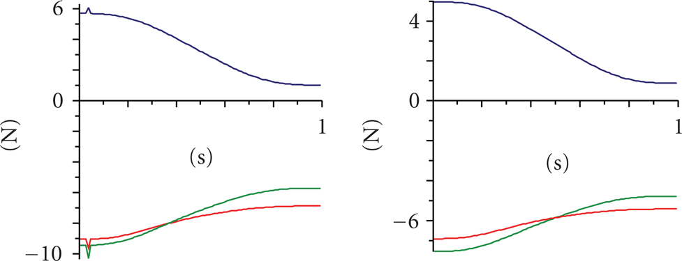
Torques values to the actuators, with constant external forces on the left and function of the time on the right: blue: the first leg; red: the second; green: the third one.

Figure 14 describes how the torques change by applying constant external forces but different motion profiles: the presence of random noise, in the right diagram, does not introduce rough behavior unlike the (a) profile of the left graph.

The hinges compliance is analyzed in Figure 15: on the left, the simulations results obtained implementing the type 1 model present higher torques values required to the actuators, confirming the stiffer behavior that this kind of hinge offers to the motion, under the same work conditions and geometrical parameters.

Figure 16 shows finally the torques profiles obtained imposing on the left a constant external force and depending on the time on right.

6. Conclusions

The kinematic and dynamic analyses of a compliant PKM mesomanipulator have been described in this paper.

The functional model of the robot has been presented in the brief introduction, and then forward and inverse analytical kinematics have been detailed. In the following paragraph the singularities and the manipulator workspace have been addressed, with particular attention to the physical reachability of the singularity conditions.

Once defined the kinematics, the dynamic problem has been delineated, under the hypothesis of lumped elasticity into the flexure hinges.

Finally, some simulations results have been presented, to compare how the actuators torque profile changes with the external imposed conditions: various motion profiles, different flexure hinges models, or a particular external force profile.

To complete the mesomanipulator analysis, an optimization of the robot scale and dimensions could be performed; the simulations results underline also the significant influence of the flexure hinges on the manipulator performance, so that particular attention should be paid to the material properties of such elements and their design. Once implemented these considerations, the manipulator analysis could be improved by considering also vibrations to evaluate the realism of the results until now obtained.

Footnotes

Acknowledgments

The authors are grateful to Diego De Santis for the interesting discussion and the contribution on the flexure hinges behavior and to the anonymous reviewers for their kind suggestions.

References

El-Khasawneh

B. S.

and Ferreira

P. M.

, “Computation of stiffness and stiffness bounds for parallel link manipulators,” International Journal of Machine Tools & Manufacture, vol. 39, no. 2, pp. 321–342, 1999.

Howell

L. L.

, Compliant Mechanisms, John Wiley & Sons, New York, NY, USA, 2001.

Craig

J. J.

, Robotics. Mechanics and Control, Addison Wesley, Reading, Mass, USA, 1986.

Hebesacker

Treib

Zirn

, and Honegger

, “Hexaglide 6 dof and triaglide 3 dof parallel manipulators,” in Parallel Kinematic Machines: Theoretical Aspects and Industrial Requirements, pp. 345–355, Springer, Berlin, Germany, 1999.

Amici

Borboni

Magnani

P. L.

, and Pomi

, “Kinematic analysis of a compliant, parallel and three-dimensional mesomanipulator generated from a planar structure,” in Proceedings of the 2nd European Conference on Mechanism Science (EUCOMES '08), pp. 479–485, Cassino, Italy, November 2008.

Erdman

A. G.

and Sandor

G. N.

, Mechanism Design: Analysis and Synthesis, Prentice Hall, Englewood Cliffs, NJ, USA, 1991.

Legnani

and Riva

, “Kinematics of modular robots,” in Proceedings of the 7th World Congress on Theory of Machines and Mechanisms (IFToMM '87), Seville, Spain, 1987.

Kong

and Gosselin

C. M.

, “Type synthesis of 3-DOF PPR-equivalent parallel manipulators based on screw theory and the concept of virtual chain,” Journal of Mechanical Design, vol. 127, no. 6, pp. 1113–1121, 2005.

Featherstone

, “Position and velocity transformations between robot end-effector coordinates and joint angles,” International Journal of Robotics Research, vol. 2, no. 2, pp. 35–45, 1983.

10.

Zhao

J.-S.

Chen

Zhou

Dong

J.-X.

, and Feng

Z.-J.

, “Workspace of parallel manipulators with symmetric identical kinematic chains,” Mechanism and Machine Theory, vol. 41, no. 6, pp. 632–645, 2006.

11.

Angelico

, and Sinatra

, “Tripod dynamics and its inertia effect,” Journal of Mechanical Design, vol. 127, no. 1, pp. 144–149, 2005.

12.

Gallardo

Rico

J. M.

Frisoli

Checcacci

, and Bergamasco

, “Dynamics of parallel manipulators by means of screw theory,” Mechanism and Machine Theory, vol. 38, no. 11, pp. 1113–1131, 2003.

13.

Wang

S.-C.

Hikita

Kubo

Zhao

Y.-S.

Huang

, and Ifukube

, “Kinematics and dynamics of a 6 degree-of-freedom fully parallel manipulator with elastic joints,” Mechanism and Machine Theory, vol. 38, no. 5, pp. 439–461, 2003.

14.

Dassa

, Mechanisms based on flexure articulations, Ph.D. thesis, University of Brescia, Brescia, Italy, March 2009.

15.

Antonini