
Abstract
Effectiveness and efficiency of hydro-cyclone separators are highly dependent on their geometrical parameters and flow characteristics. Performance of the hydro-cyclone can, therefore, be improved by modifying the geometrical parameters or flow characteristics. The mining and chemical industries are faced with problems of separating ore-rich stones from the nonore-rich stones. Due to this problem a certain amount of precious metals is lost to the dumping sites. Plant managers try to solve these problems by stockpiling what could be useless stones, so that they can be reprocessed in the future. Reprocessing is not a sustainable approach, because the reprocessed material would give lower yield as compared to the production costs. Particulate separation in a hydro-cyclone has been investigated in this paper, by using computational fluid dynamics. The paper investigated the influence of various flow and geometric parameters on particulate separation. Optimal parameters for efficient separation have been determined for the density of fluid, diameter of the spigot, and diameter of the vortex finder. The principal contribution of this paper is that key parameters for design optimization of the hydro-cyclone have been investigated.
1. Introduction
The separation of dispersed solid particles from a suspension is an essential unit operation in many fields of mechanical separation technology, for instance mining and chemical industries. Typical apparatuses used are filters, centrifuges, and hydrocyclones. Whereas an enormous energy input is necessary when using centrifuges at a high rotational speed, hydrocyclones work more economically, as the only amount of energy which has to be supplied is to overcome the pressure drop. A further advantage of hydrocyclones is their high operational reliability, as they are simple in construction without any moving parts. Despite its ubiquitous applications in the chemical, metallurgically and other industries, the hydrocyclone still requires specific investigation since the flow field is not completely understood. Fisher and Flack [1] published experimental studies of the flow in hydrocyclones. This has been informative with regards to the internal flow-field dynamics, but the following important aspects are still not understood.
The frequently reported but anomalous “fish-hook” effect, which results in an excess of fines reporting to the underflow, has not been categorically explained.
Hydrocyclone modelers have largely ignored features such as the nature of air-core development, with simplified air-core assumptions being made.
Detailed knowledge of the flow structure is required if one is to consider such issues as energy saving, cost, economy, or product quality. Several benefits could arise from this knowledge, for instance, areas of high erosion may be identified and potentially minimised or accounted for in design, design modifications for improved separation or reverse design of cyclone geometry could be obtained.
The drivers behind the application of simplified physical models of hydrocyclone behaviour are principally the issues of complex flow behaviour arising from the three-dimensional flow entry, multiphase interactions, and the mechanisms governing the formation of an air core (when the hydrocyclone is open to the atmosphere). Computational fluid dynamics modeling technology is not yet perfect in modeling hydrocyclones, and it is certainly still possible to improve our understanding of the fundamentals and models needed to describe them. Nevertheless, computational modeling techniques are being used to compare and understand the workings of different hydrocyclone designs and models. Consequently, computational studies have been, in general, limited to low particle-concentration flows and to simplified geometries of the hydrocyclone entry region. Advanced theoretical and experimental techniques are still needed to obtain a better understanding of the very complex physical phenomena affecting the performance of hydrocyclones. The knowledge of phenomena such as particle-particle, particle-fluid, and particle-wall interactions would open the way to the description of particle effects for suppression or generation of turbulence and for non-Newtonian slurry flows.
The hydrocyclone suffers from two inherent deficiencies. The first one is the coarse particle bypass whereby coarse particles in the feed stream move along the boundary layer over the vortex finder and hence directly join the overflow stream. The second one is fine particle bypass. This is unavoidable in the sense that very fine particles do not possess sufficient drag force to resist moving with the fluid medium. Thus, the amount of fines reporting to the underflow is nearly equal to the fraction of feed water reporting to the underflow [2]. The only way to minimize the bypass fraction is to reduce the amount of water passing through the underflow, which is accomplished by increasing the centrifugal force so that the underflow stream is highly concentrated with solids. Thus, in the design of hydrocyclone, the two bypasses must be minimized to realize higher performance efficiencies.
This study involves the simulation of flow in a hydrocyclone in order to improve its performance. The objective of the work is to investigate, using computational fluid dynamics, (CFD) the influence of flow and geometric parameters on separation of solids and liquid. This study attempts to minimize both underflow and overflow bypasses in order to realize higher performance efficiencies.
2. Nature of the Problem
The hydrocyclone of the base model (Figure 1) is composed of an inlet pipe of a 255 mm diameter which makes a volute on the cylinder of the cyclone. The cyclone cylinder has a diameter of 800 mm and a length of 800 mm. It has a cone of 500 mm length and a cone angle of 20 degrees. The cone is open at the spigot, with a cylinder of 100 mm length and 320 mm diameter. The vortex finder is a cylinder of 1050 mm length and 488 mm diameter. The inlet pipe connects to the cylinder in volute manner in order to minimize turbulence where cylinder flow and the inlet pipe flow meet and is more efficient compared to other types. The cyclone has to separate copper particles from stones using gravitational feed. Ideally, copper particles should exit through the spigot, while the stones and fluid exit through the vortex finder. The case for now is that some copper-particles exit at the vortex finder at an unexpected rate. While, engineers tried to control this by varying the density of the fluid medium, more stones exit through the spigot. The problem had to be investigated to find the ideal geometric parameters and flow conditions for satisfactory separation. As it is expensive to perform parametric optimization experimentally, computational fluid dynamics became the most relevant tool for the study.
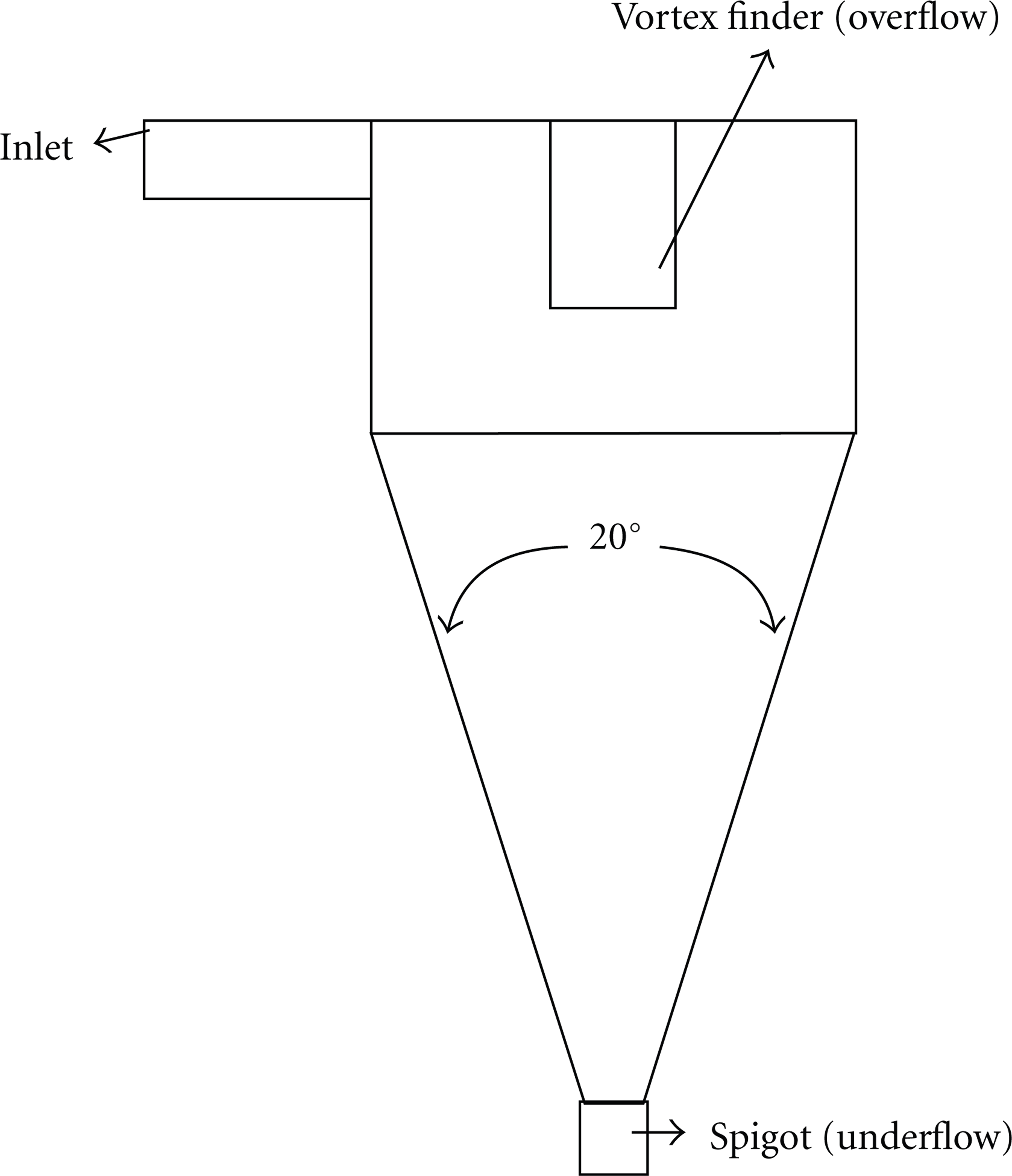
A schematic diagram of hydrocyclone geometry.
3. Numerical Simulation
A segregated, steady state, 3D double-precision implicit solver was used for simulating the flow and turbulence inside the hydrocyclone. The pressure-interpolation scheme adopted was PRESTO (pressure staggered option), which is useful for predicting highly swirling flow characteristics prevailing inside the cyclone body [3]. In order to reduce the effects of numerical diffusion, higher-order discretization schemes are recommended for simulating cyclones. Accordingly, a third-order accurate QUICK scheme was used for spatial discretization. The SIMPLE algorithm was used for coupling the continuity and momentum equations. Turbulent flow inside a hydrocyclone is anisotropic in nature, hence choice of turbulence model is crucial. Within the framework of RANS family, the Reynolds stress model (RSM) is known to predict turbulence behavior inside a cyclone with a better accuracy [4]. Thus, in the present study, RSM was chosen. It was observed that RSM required large number of iterations (about 7500 to 8000) for the solution to stabilize. This method of simulation has implicitly generated the low-pressure core around the cyclone axis without any additional definitions for air core. For achieving the particle-separation behavior inside the cyclone, the discrete phase modelling (DPM) technique was adopted.
This method simulates the particle trajectory in a Lagrangian frame of reference. The stochastic tracking model was adopted for the dispersion of particles due to turbulence in the primary phase. The discrete phase formulation used in Fluent contains the assumption that the second phase is sufficiently dilute that particle-particle interactions and the effects of the particle volume fraction on the primary phase are negligible. In slurries with dilute concentrations of solids (particle concentration below 15% by weight), particle-distribution behavior can be simulated using Lagrangian particle-tracking approach. Thus, in the present study particle tracking is carried out using the above methodology. Steady state was achieved after 1200 iterations, at which time the residuals and flow rates were constant. After the steady state was reached, a real time of 1 s was simulated with time steps of 0.0005 s. An average of over 1000-time steps were taken to record the velocity profiles, mass balance and flow rates. A sample of 2400 particles in each size fraction was injected at the inlet and tracked down the flow until each particle left through the outlets. The slurry used is one of 7.5% by wt of both copper particles and stones. From the particle trajectory the cumulative distributions were computed as the split ratio for each size class. The mass balance is primary in the analysis of the hydrocyclone performance. In the exploration of novel designs, these values determine the improvement of the process. The mass balance was computed from the particle trajectory for each size fraction.
4. Meshing Scheme
Hydrocyclones truly cannot be modeled in a 2D plane due to nonaxisymmetric nature at the feed inlet opening. Earlier reports also indicated that the results using a 3D model are better matching with the experimental data compared to the results with axisymmetric geometry. The present computational model is based on 3D geometry. Triangular mesh, which can fit into small acute angles in the geometry, is used to mesh the face that joins the inlet to the cylindrical cyclone body. This triangular mesh is then extruded in the vertical direction to give rise to wedge-shaped control volumes in the tangential inlet region. The rest of the cyclone is meshed using unstructured hexahedral mesh, which is known to be less diffusive compared to other types of meshes like tetrahedral. Since there is a high degree of repetitiveness in a CFD study, the whole CFD process was automated that is, geometry modeling, mesh generation, and boundary conditions definition. Parametric studies were carried out by enabling evaluation of several combinations of design variables.
A boundary-layer mesh is generated adjacent to the outer wall of the cyclone. In order to capture the low-pressure central air-core, block-structured mesh is generated in that region. Air is drawn in at the spigot and exits through the vortex finder via a stable air core. For modeling the air core a two-fluid modeling approach is normally applied, but the RSM model has also been proven to give better accuracy in modeling the air-core and flow turbulence [5]. For the above reasons, an RSM model has been used in this work. Additional care is taken to generate mesh near the spigot region where maximum aspect ratio is restricted to about 10. This is important to capture the back flow through spigot opening. Grid independence study was carried out with five different mesh densities with mesh sizes varying from 200,000 to 600,000. Water distribution studies have indicated that better predictions are obtained at higher mesh densities. A mesh density of 600,000 cells is optimized due to good predictions and reasonable computational time for simulations.
5. Boundary Conditions
The continuous phase was a mixture of water and a ferromagnetic powder with a density of 2850 kg/m2. The other phase (solid/particles) comprised of copper and stones. Copper has a density of 4000 kg/m2, and stones have a density of 1800 kg/m2. The two-phase flow enters the hydrocyclone by the inlet pipe, and this boundary was used as a mass-flow-inlet boundary condition. Due to separation in the hydrocyclone, the flow was divided in two parts, one went to the spigot and the other went to the vortex finder. The boundary conditions of a face at the bottom of the vortex finder and a face at the spigot where the flow went out are prescribed as pressure outlet boundaries.
6. Experimental Validation
Experiments were carried out with a hydrocyclone having a geometry the same as the one used for the computational work. The cyclone was inclined at an angle of 15° and gravity fed with pressure of 260 kPa. The vortex finder length was varied during the tests. For each experiment, samples were collected from the vortex finder (overflow) and the spigot (underflow) streams. Three experiments were performed for each vortex finder length, and the results were averaged. The samples were characterised according to whether the material is copper or stones. After characterisation, the individual particles were counted in order to calculate the separation efficiency. In this experiment, copper was expected to exit through the spigot and stones through the vortex finder. The last experiment was performed on the optimised model to find its separation efficiency.
7. Vortex Finder Length
The results of a base case design from simulation studies as shown in Figures 2(a), 2(b), and 2(c) show static pressure, axial velocity, and copper and stone trajectories. The static pressure (Figure 3(a)) inside the system decides the material flow in the radial and vertical direction within the hydrocyclone. It can be observed form the figure that the pressure values are minimum near the central axis and maximum on the hydrocyclone walls. The lowest pressure is negative, and it is expected that zero pressure and below indicatez the existence of the air core.

Base case design analysis of a hydrocyclone.

Contours of static pressure, velocities, and trajectories of solid particles at various vortex finder lengths.
Figure 3(b) shows the contours of axial velocity for the base case design. In the Figure, positive values indicate, flow towards the vortex finder (upward), and negative values indicate flow towards the spigot (downward). Higher positive velocities are visible within and in front of the vortex finder. While negative velocities are visible at the spigot. Figure 3(c) shows both copper (left) and stones (right) characterization. In this figure, both copper and stones are visible at the two ends and that indicates inefficient separation.
The standard model has a 488 mm vortex finder length. The vortex finder length will only be increased because as the inlet pipe curls around the cylinder to create a volute, it covers nearly 488 mm of the cylinder length, and if the length of the vortex finder is decreased, flow from the inlet pipe will go directly into the vortex finder. This modification is proposed to reduce the bypass or short circuiting of coarse particles through the vortex finder [6]. The coarse particles have a tendency to reach the vortex finder wall directly from the feed inlet [7]. Then, they travel downward along the vortex finder wall and are caught in the upward flow through the vortex finder. Thus, coarse particles take a shorter path to the overflow. The expectation is that the widening cylinder would distance the coarse particles from the vortex finder.
Figure 3 shows contours of static pressure, axial velocity, and trajectories of solid particles for various vortex finder lengths. The figures show a similar trend in static pressure for all five vortex finder length iterations. Higher axial velocities are visible within and in front of the vortex finder while lower velocities are at the spigot. The problem is that when the length of the vortex finder is too big (950 mm), trajectories of copper particles reappear at the vortex finder. For this investigation, a 900 mm vortex finder length is the ideal for efficient separation of solid particles, because all copper particles go out through the spigot and less stones appear in the spigot. According to Martínez et al. [6] optimum length depends on feed-particle size and distribution, and this should be determined preferably by experimentation. There is no complete agreement on vortex finder length due to the fact that this depends on geometry, feed-particle size, and feed concentration. There are several values recorded in the bibliography that express the ratio of the length of the vortex finder to the hydrocyclone diameter. Elimination of short circuit by means of a vortex finder; the case of Rietema [8] who gives a value of 0.4; Bradley [9] and Haas et al. [10] propose a figure of 1/3, Wang and Yu [11] accept as valid a value of 0.67; Narasimha et al. [5] use two values (0.67 and 0.5). Kraipech et al. [12] juggled with different vortex finder insert depths, but for different hydrocyclone geometries, obtaining ratios ranging from 0.28 to 0.93.
The results in Figure 3 were validated against experimental results, so that correctness of simulated results can be ensured. The results for validation are shown in Figure 4. The results basically indicate that 40% (simulated) and 45% (experimental) of copper exit through the vortex finder. The results also indicate that 56% (simulated) and 62% (experimental) of stones exit through the spigot. The optimal vortex finder length was achieved at iteration 4, with vortex finder length of 900 mm (Figure 3). Both the simulated results and experimental results have low values in the vicinity of vortex finder length of 900 mm.
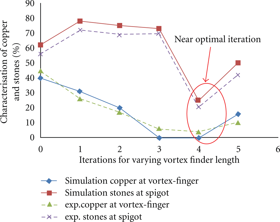
Experimental validation of CFD model of hydrocyclone for varying vortex finder lengths.
For this validation study, the experimental results follow the simulated results closely, indicating that the simulated results can be relied upon. Therefore, the entire parametric study will be performed with simulations because it will be quicker and cost effective to use. However, the final design will also be validated.
8. Variation of Fluid (Medium) Density
In this case, the density of the fluid (medium) was varied. The industry used a density of 2850 kg/m2 and diameter of 25 mm for both copper particles and stones. The density was varied to see its consequence on the flow separation. Figure 5 shows the simulation results for the base case. It can be observed from Figure 5 that the pressure values are minimum near the central axis and maximum on the cyclone walls with progressive concentric layers of increasing pressures from core to the cyclone wall, and this shows a favourable pressure gradient. It can also be observed from the figure that the pressure contours are more or less axissymmetric around the cyclone axis, covering a large cyclone height. However, some kind of asymmetry is observed at vertical heights approaching the spigot opening. The static pressure inside the system basically decides the material flow in the radial and vertical direction within the cyclone. The axial velocities have similar trends, and show that flow-in around the vortex finder is upward and flow-in around the spigot is downward.
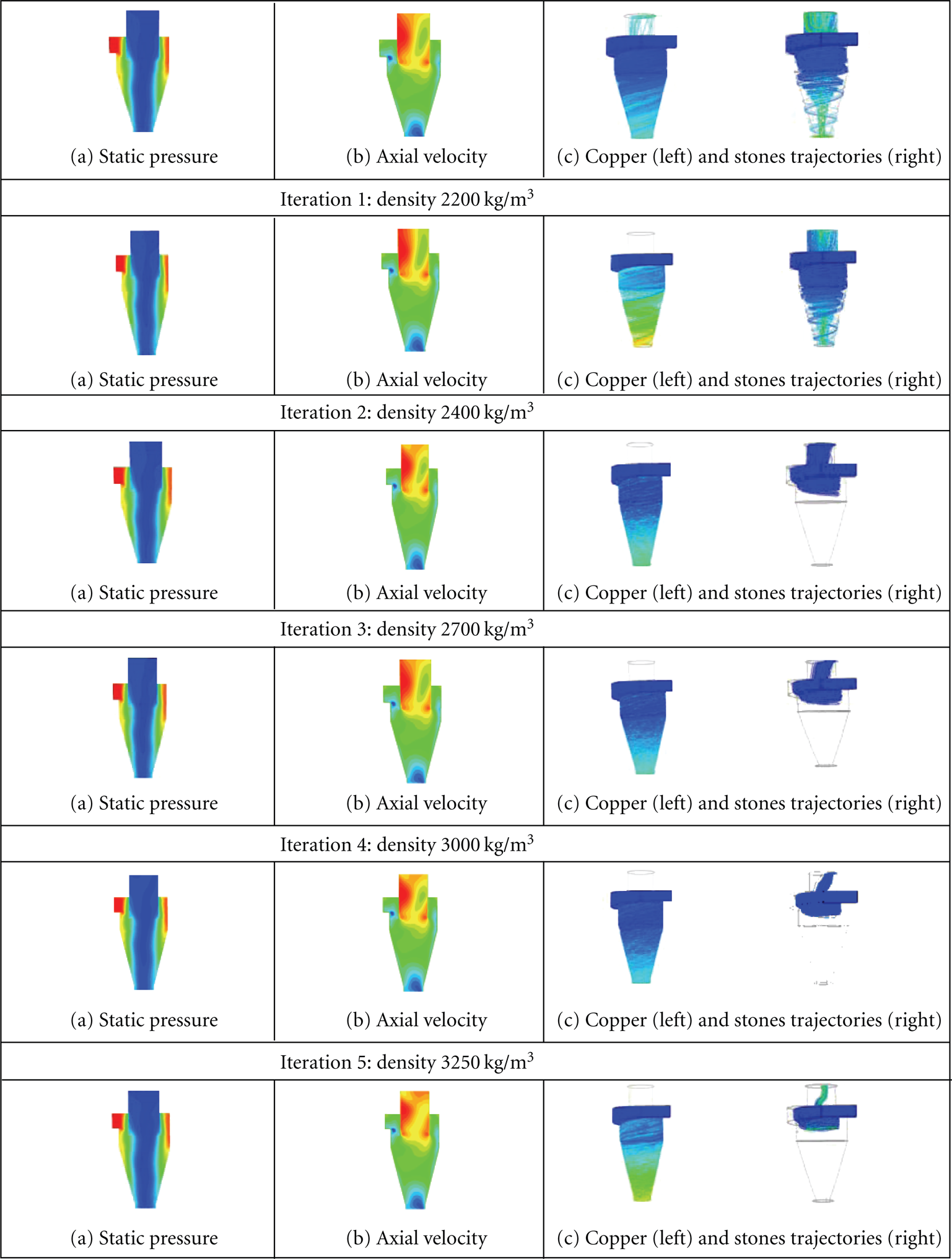
Contours of static pressure, velocities, and trajectories of solids at various fluid densities.
Figure 5 also shows trajectories of copper particles (left), and stones (right) for the base case model. It is clear that this cyclone is not effective in classifying the flow material. Some trajectories of copper particles are visible at the vortex finder (left), and this is undesirable. Also, some trajectories of stones (right) are visible at the spigot, and while it is not desirable, it is common because the rest of the stones will be removed by the next stage of separation.
Figure 5 shows the results of variation in the fluid density. In all the iterations, the static pressure is low in the middle, indicating favourable conditions for separation, but that might not be interpreted as ideal for efficient separation. This condition, though not the same for all the iterations, provides favourable conditions for separation of copper particles and stones. But, as the density increases, the lower pressure region increases outwards weakening the separation of solids. At a density of 3250 kg/m2 copper particles appear at the overflow. This density is, therefore, not recommended because copper particles would be lost to damping site. The tangential velocity, like the pressure, has a central cyclone of low velocity (in red) and high velocity at the entrance of the flow (blue). The tangential velocity increases when the density decreases. So the acceleration force is higher than the pressure force when the density decreases, and at 2200 kg/m2 stone particles appear at the spigot. When the density of the continuous phase gets near the stones’ density, stone particles appear at the two outlets, and when the continuous phase density gets near the copper density, copper particles appear at the two outlets. The best is to take density in the vicinity of 3000 kg/m2.
9. Diameter of Particles
The base case diameter of copper and stones is around 25 mm. In this case, diameters of copper particles and stones were varied in order to observe how this variation affects separation of the two. From Figure 6, it can be seen that near optimal diameter is 10 mm, because beyond 10 mm and after 5 mm, trajectories of solids appear at unintended outlets. Fine particle bypass (below 5 mm diameter) is unavoidable in the sense that very fine particles do not posses sufficient drag force to resist moving with the fluid medium. According to Svarovsky [2] the amount of fines reporting to the underflow is nearly equal to the fraction of feed water reporting to the underflow. The only way to minimize the bypass fraction is to reduce the amount of water passing through the underflow, which is accomplished by increasing the centrifugal force so that the underflow stream is highly concentrated with solids.

Trajectories of solids particles at various particle diameters.
10. Volume Fraction
The proportion between the continuous phase and the discrete phase is investigated here. The software limits the proportion of the discrete phase to continuous phase to within 10–15%. So the proportion of the discrete phase was varied between 0.5 and 15%.
Figure 7 shows some dependence of particle separation on the volume fraction of particles. However, Figure 7 indicates that as the volume fraction decreases, copper particles effectively decrease for volume fraction higher than 10%, but for stones the results are inconclusive. The CFD model used is only limited to 15% volume fraction, beyond that the results would be unrealistic. So we can use a volume fraction of 10%. A very dilute slurry would be preferable, but that would impact on the throughput of the process.
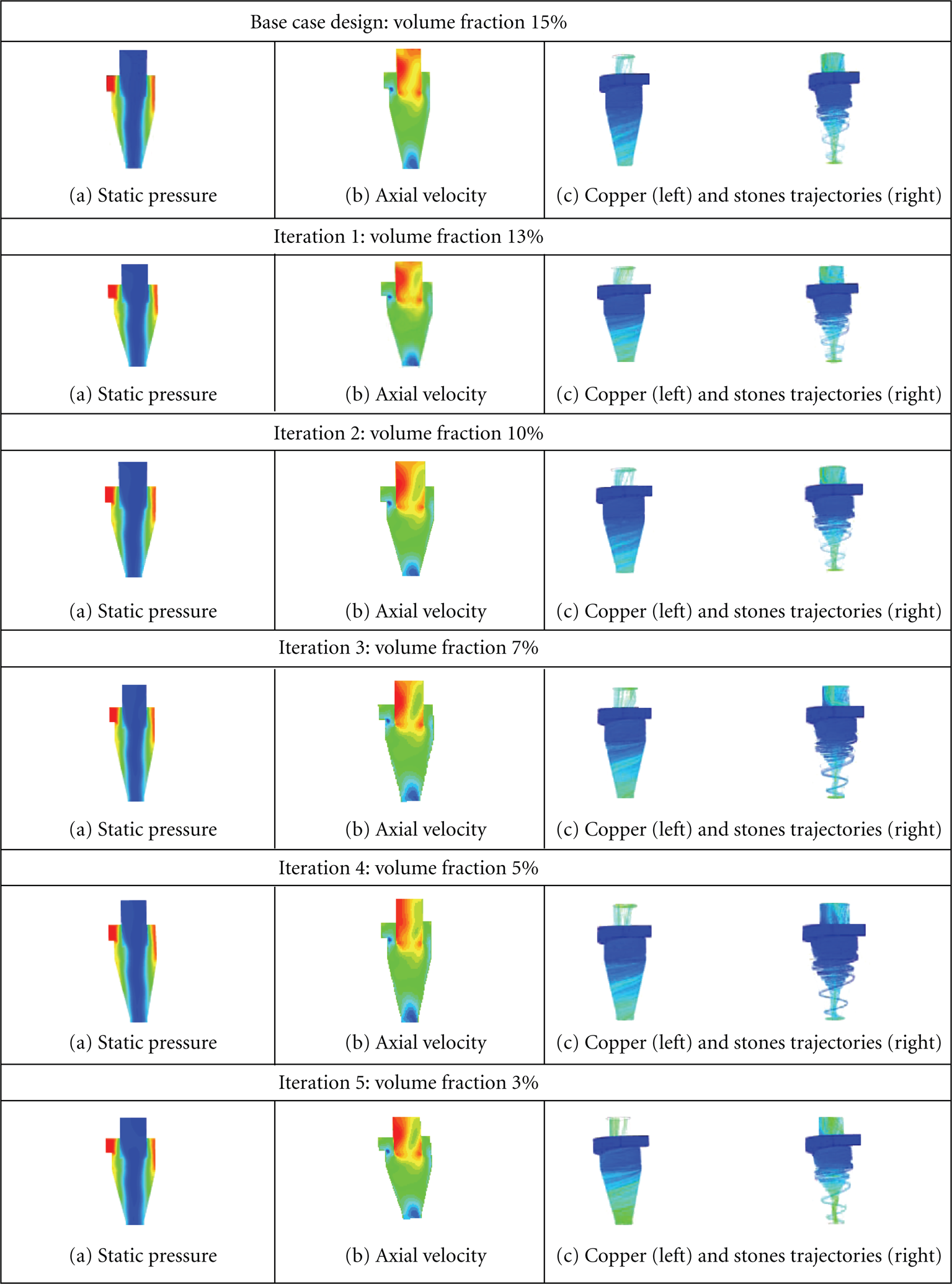
Contours of static pressure, velocities, and trajectories of solid particles at various flow volume fractions.
The accumulation of solid particles in regions of high fluid-strain rate and low vorticity can result in high values of the local particle concentration, indicating the presence of a significant (local) coupling of the two phases. When solids concentration exceeds 5% by volume, the presence of particles changes the viscosity stresses and results in the generation of the extra inertial stresses. The former can be described by introducing a slurry mixture viscosity as the function of particle concentration [13]. The latter, known as the Bagnold dispersive stresses, result from particle-particle collisions, which are important when particle concentration exceeds 10% by volume. In the case of shearing particles of mixed size, the larger particles drift towards the zone of least shear strain, for example, towards the hydrocyclone axis, and the smaller particles towards that of greater shear strain, for example, to the wall. Consideration of the Bagnold stresses might prove useful for explaining “fish-hook” effect, of Haas et al. [10] the which was also reported by Wang and Yu. [11] amongst others.
11. Variation of Vortex Finder Diameter
The vortex finder diameter of the standard hydrocyclone is 488 mm. In this case, the effects of variation of vortex finder diameter on particle separation were investigated.
Figure 8 shows contours of static pressure and trajectories of solid particles at vortex finder diameter. The figure indicates that when the vortex finder diameter is increased, the contours of total pressure get distorted. The lower pressure is no longer along the central axis, and this caused poor separation. It can be observed at iteration 2 that at a diameter of 450 mm, the same flow distortions are evident, and had caused all stones to go to the spigot. Hence, it can be concluded that the optimal diameter of the vortex finder is in the vicinity of 488 mm.
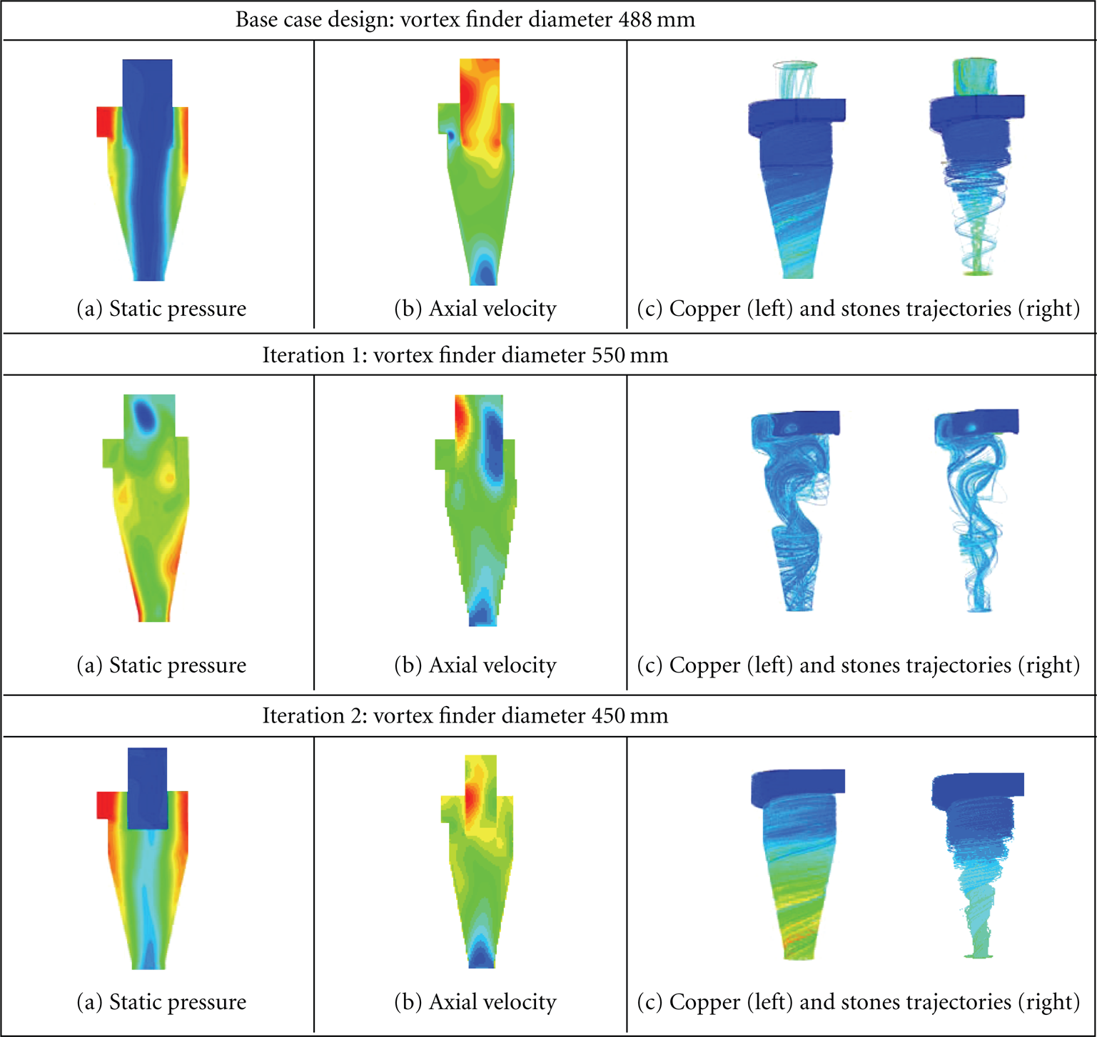
Contours of static pressure, velocities, and trajectories of solid particles at vortex finder diameters.
12. Spigot Diameter
The standard spigot diameter is 320 mm. In this case, the effect of spigot diameter on particle separation was investigated. The cone angle remained constant, while the length of the cone was increased to accommodate varying spigot diameters. Figure 9 shows contours of static pressure and trajectories of solid particles at various spigot diameters.
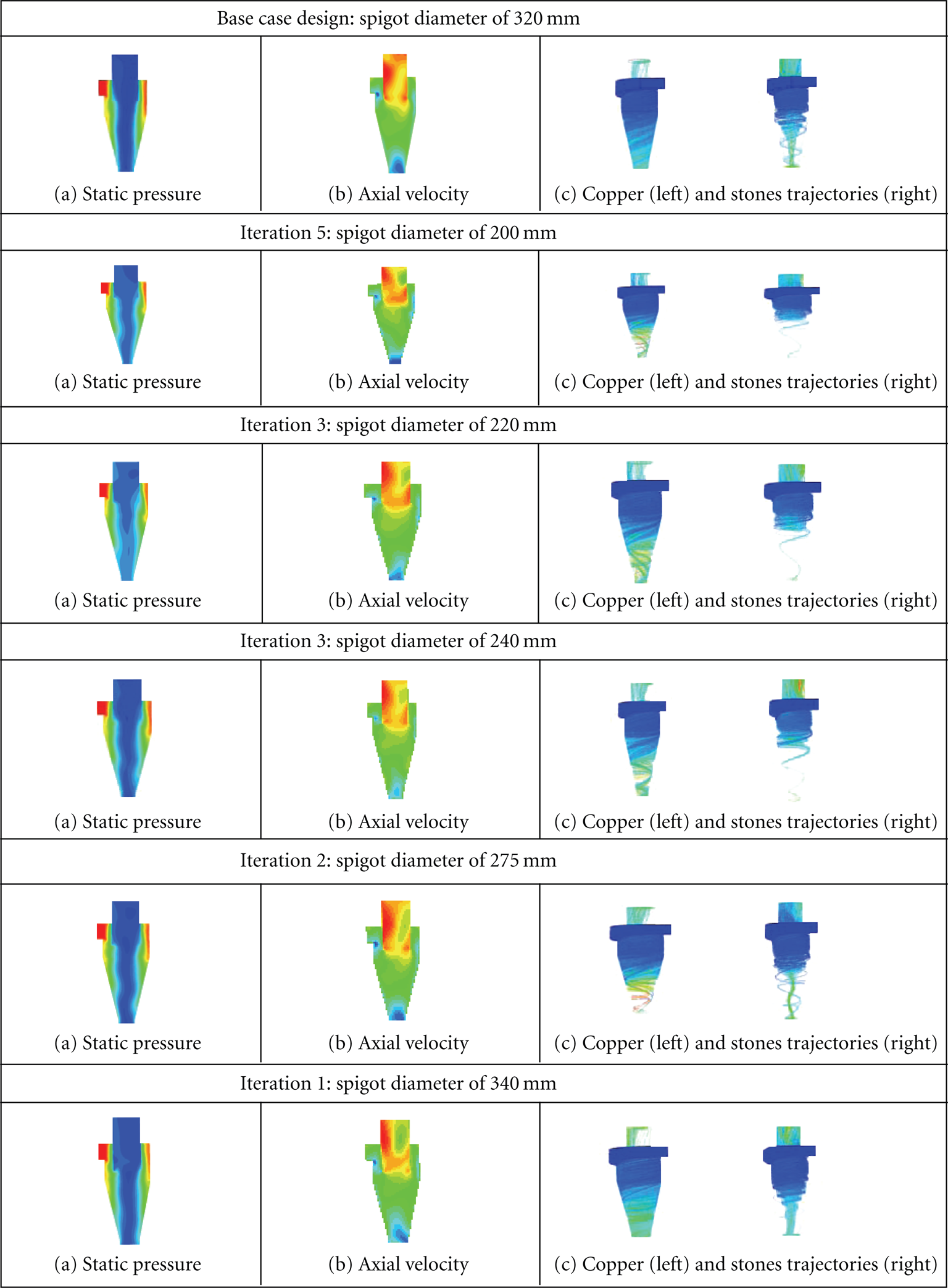
Contours of static pressure, velocities, and trajectories of solid particles at various flow volume fractions.
Figure 9 shows that as the diameter of spigot is decreased, the thickness of the low-pressure zone in the axis of the hydrocyclone decreases. The stones in the spigot decreased as the spigot diameter decreased. The number of copper particles is lower for a diameter of 320 mm. The best spigot diameter is in the vicinity of 320 mm.
13. Final Result
This case investigated the performance of the hydrocyclone with parameters determined to be near optimal. The spigot diameter is 320 mm, the vortex finder length is 900 mm, and the vortex finder diameter is 488 mm (original diameter). The density of the continuous phase is 2850, and the volume fraction is 10%. The diameter of both copper particles and stones was 25 mm. The optimized design has achieved higher separation efficiencies that is, 100% copper (simulated) and 93% copper (experimental) and 92% stones (simulated) and 85% stones (experimental).
Figure 10 shows the contours of pressure and trajectories of solids for the proposed design. In this model, in the low-pressure zone the symmetry of the hydrocyclone that promotes separation exists. All the trajectories of copper particles appear at the spigot, and a few trajectories of stones appear at the spigot. This indicates better performance as compared to the original design.
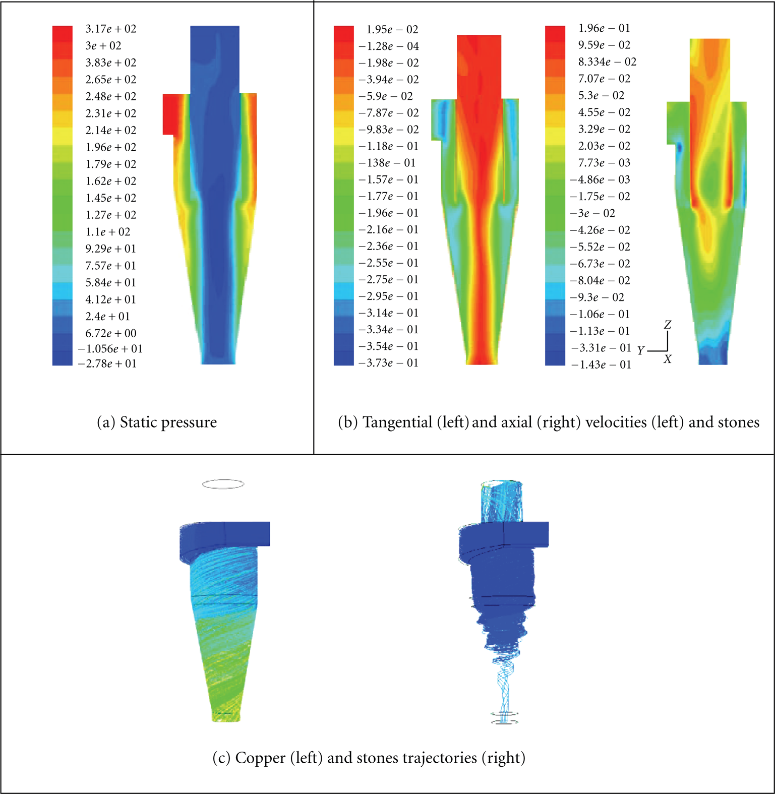
The proposed hydrocyclone model.
14. Conclusion
From the results, it can be concluded that separation in hydrocyclone is still a problem. Getting optimal performance is a real challenge, and plant managers cannot easily decide whether to dump the stones or stockpile them for further recycling. While CFD can be used to assess designs before installation and troubleshooting, the modeling procedure is difficult because of everchanging boundary conditions. The following paragraphs summarize the results of the simulations performed on the hydrocyclone.
When the density of the fluid approaches that of the stone, stones appear in the spigot, and when it approaches that of the copper particles, copper particles appear in the vortex. The above cases are undesirable for efficient separation of stones from copper particles. Optimal density for separation has been found to be in the vicinity of 2900 kg/m3, and that makes the original density (2850 kg/m3) sufficient.
The volume fraction was not shown to be have an influence on separation of stones and copper for 5 to 15% volume fraction. It is, however, recommended that for efficient separation of slurries and for the CFD model to perform well, the volume fraction of particles must be less than 15%.
The near optimal length of the vortex finder for efficient separation has been found to be in the vicinity of 900 mm. Increasing the vortex finder length, more time is given for particle re-entrainment in the underflow stream, and this increases separation efficiency. Nonetheless, if the vortex finder tip reaches the conical zone, some coarse particles might reach the return overflow stream instead of exiting through the apex, and this causes a decrease in efficiency.
The optimal diameter of the vortex finder for efficient separation has been found to be in the vicinity of 488 mm. This case was also investigated for particles of 1 mm diameter.
The near optimal diameter of the spigot for efficient separation has been found to be in the vicinity of 320 mm.
The near optimal design was found to have a vortex finder length of 900 mm and a vortex finder diameter of 488 mm. The model was investigated with variations of particles diameters, while all geometric and flow parameters were left unchanged. This model performed better for all particle diameters more than 1 mm.
In general, it can be concluded that due the complexity of the fluid dynamics within a hydrocyclone, the performance of hydrocyclones should be treated on case-by-case basis. Computational fluid dynamics is the best tool for analysis of multiple models. This paper has revealed important parameters to be considered for improving performance of the hydrocyclone and, to some extent, search directions for optimal parameters.