Sage Journals: Discover world-class research

Abstract

This paper provides a method to determine the variable flexible joint parameters which are dependent on configurations for a PRS Parallel Robot. Based on the continuous force approach, virtual springs were used between the joint components to simulate the joint flexibility. The stiffness matrix of the joint virtual springs was derived. The method uses system dynamic characteristics in different configurations to set the virtual spring stiffness for all the joints in the system. Modal testing was conducted on a set of selected robot configurations to determine the system natural frequencies and mode shapes along with their variation. To obtain the virtual spring stiffness, the system was condensed at the joint nodal coordinates. Then eigen-sensitivity analysis was conducted on the condensed system matrices with respect to the stiffness parameters of the joint virtual springs. Thus, the virtual spring parameters in the model can be set to match the variation of the system dynamic responses with the robot configuration changes. The virtual spring parameters between the selected robot configurations were obtained by interpolation. The research indicates that the method is effective and relatively easy to conduct, compared to other methods. The variable flexible joint model is applicable to flexible multibody systems with variable configurations.

1. Introduction

Dynamic modeling of flexible multibody systems is a classical problem. The link flexibility and joint compliance (elasticity) of robots or mechanisms in general have been studied for a long time. This paper focuses on the difficult issue of joint flexibility which varies due to system configuration changes. Joint flexibility has been studied since the 1980s, mainly by relating it to contact/impact mechanics. Tzou et al. [1] proposed a stochastic approach to model the random feature of the dynamic contacts in the joints. Bowden and Dugundji [2] presented the linear and nonlinear analysis for the global dynamics of jointed structures. Moon and Li [3] conducted an experimental study on a pin-jointed truss. Tzou and Rong [4] provided a mathematical model for a three-dimensional spherical joint based on the contact force analysis. Kakizaki et al. [5] presented a dynamic modeling method for a SCARA manipulator with link flexibility and joint clearances. Seneviratne et al. [6] provided a combined massless-link and spring-damping model for modeling the joint clearance. Ravn et al. [7] presented the analysis of revolute joint clearances with and without lubricant. Schwab et al. [8] presented a study on the dynamic response of mechanisms affected by the joint clearance. Ting et al. [9] presented a novel and simple approach to identify the worst position and direction errors due to the joint clearance of a single loop linkage. Zhu and Ting [10] studied the uncertainty of planar and spatial robots with joint clearances. Wang et al. [11] presented the virtual spring method at joints to completely decouple the dynamic model of complex robotic systems with closed kinematic chains.

In the above investigations, two basic approaches were used in the dynamics of flexible joint systems. The first approach uses an impulse momentum model, where the pieced intervals are analyzed. The impulse momentum equations can be solved with the restitution condition for the jump discontinuity in the system velocities and the joint reaction forces. The second approach uses a continuous force model to represent the force of interaction between the impact surfaces. Stiffness and damping coefficients are set to account for the impact surface compliance and energy dissipation during the impact process. Obviously, the second approach is easier to handle than the first. No matter which method is used, a key step is to determine the parameters in the joint models. Though the above models are effective to different extents when used to represent the physics of an individual joint in a configuration-fixed system, they are difficult to use for multiple joints assembled together in a configuration-variable system (such as a robot). The difficulty is that the joint flexibility parameters may change when the system configuration changes. Also, the parameters may be different for the same type of joints at different locations in a system. It is the highlight for this paper to display how to set the flexibility parameters for multiple joints in a system with variable configuration.

Based on the continuous force model, this paper presents a modeling method on the joint whose flexibility results from the variable joint looseness due to the system configuration change. The flexible joint model was used in the simulation of a PRS parallel robot shown in Figure 1. Instead of studying the joint individually, the method uses system dynamic characteristics to set the flexibility parameters for all the joints in the system. Experimental modal testing was conducted at a set of selected robot configurations to determine the variation of the system natural frequencies and mode shapes. To easily obtain the joint flexibility parameters, the system was condensed at the joint coordinates. At each selected robot configuration, eigen-sensitivity analysis was conducted on the condensed system matrices with respect to the joint flexibility parameters. Thus, the joint flexibility parameters in the model can be updated at each selected robot configuration to be consistent with the variation of the system dynamic responses. The joint flexibility parameters between the selected configurations were obtained by interpolation.

Figure 1

The Parallel Robot Prototype.

2. Flexible Joint Model

Figure 2 shows the system model of a PRS parallel robot, where OXYZ is the global reference, ${}^{p}O {}^{p}X {}^{p}Y {}^{p}Z$ is the platform body reference, and ${}^{l}O {}^{l}X {}^{l}Y {}^{l}Z$ is the leg body reference, l = 1, 2, 3. As a continuous force model, all the joint constraints are released and replaced by virtual springs and virtual dampers correspondingly, except for the rotational constraint around ^lZ in the revolute joints. Figures 3(a) and 3(b) show the flexible revolute joint model and the related coordinate system, where k_1/l, k_2/l, k_3/l, and k_4/l are the stiffness parameters of the virtual springs at the revolute joints in their original constrained directions: along ${}^{l}X {}^{l}Y {}^{l}Z$ , and around ^lX, respectively, l = 1, 2, 3. Similarly (not shown), let k_5/l, k_6/l, and k_7/l be the stiffness parameters of the virtual springs at the spherical joints in the directions of the leg body reference ${}^{l}O {}^{l}X {}^{l}Y {}^{l}Z$ : along ^lX, ^lY, and ^lZ, respectively, l = 1, 2, 3. Altogether there are 21 stiffness parameters of the joint virtual springs, or simply called joint stiffness parameters, in the robot system model. In the revolute joint, the rotational constraint around ^lZ (leg axis in undeformed state) is still kept, because releasing of this constraint is kinematically meaningless for the tripod motion (configuration determining), and the kinetic energy of this rotation is small enough to omit (compared to the rotation around ^lX).

Figure 2

Parallel Robot System Model.

(a) Flexible Revolute Joint Model (axial-section view). (b) Flexible Revolute Joint Model (cross-section view).

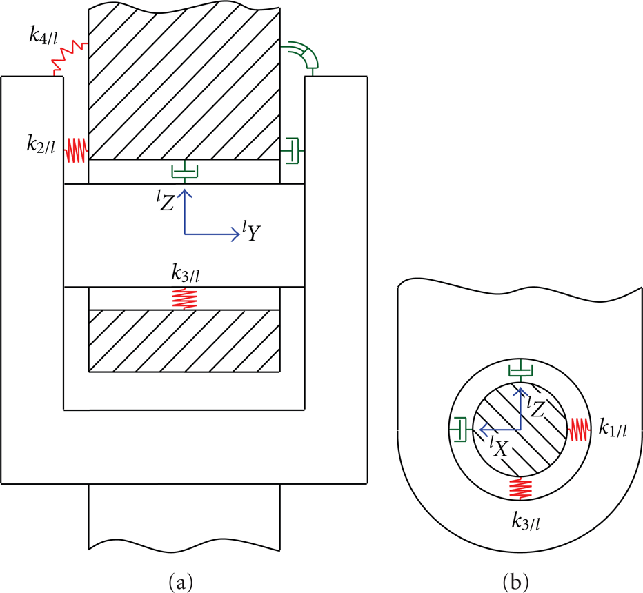
In this case it is recognized that the special revolute joint (not related to the leg body) is not a “general” revolute joint even for the flexible case, and so the symbol “R” in the phrase “PRS parallel robot” may not seem perfectly suitable. Rather than use a special symbol (such as R′), we have maintained the use of R in order to reduce unnecessary confusion. For simplicity, this research considers the joint virtual dampers with modal damping in the entire system; only the joint virtual springs are modeled here.

The potential energy of the joint virtual springs in the lth branch can be originally written as

\begin{matrix} {}^{j}{U_{l}} & = \frac{1}{2} k_{1 / l} {}^{l}{u_{R}^{2}} + \frac{1}{2} k_{2 / l} {}^{l}{v_{R}^{2}} + \frac{1}{2} k_{3 / l} {}^{l}{w_{R}^{2}} \\ + \frac{1}{2} k_{4 / l} {}^{l}{ϕ_{R}^{2}} + \frac{1}{2} k_{5 / l} {({}^{l}{u_{S}} - {}^{p /}{u_{S / l}})}^{2} \\ + \frac{1}{2} k_{6 / l} {({}^{l}{v_{S}} - {}^{p /}{v_{S / l}})}^{2} + \frac{1}{2} k_{7 / l} {({}^{l}{w_{S}} - {}^{p /}{w_{S / l}})}^{2}, \end{matrix} \begin{gathered}  \end{gathered}

(1)

where ${}^{l}{u_{R}}$ , ${}^{l}{v_{R}}$ , ${}^{l}{w_{R}}$ , and ${}^{l}{ϕ_{R}}$ are the nodal coordinates of the leg at the revolute joint of the lth branch along ^lX, ^lY, ^lZ, and about ^lX directions, respectively; ${}^{l}{u_{S}}$ , ${}^{l}{v_{S}}$ , and ${}^{l}{w_{S}}$ are the nodal coordinates of the leg at the spherical joint of the lth branch along ^lX, ^lY, and ^lZ directions, respectively; ${}^{p /}{u_{S / l}}$ , ${}^{p /}{v_{S / l}}$ , and ${}^{p /}{w_{S / l}}$ are the nodal coordinate projections in leg body reference ${}^{l}O {}^{l}X {}^{l}Y {}^{l}Z$ from ${}^{p}{u_{S / l}}$ , ${}^{p}{v_{S / l}}$ , and ${}^{p}{w_{S / l}}$ , the nodal coordinates of the platform at the spherical joint of the lth branch along ^pX, ^pY, and ^pZ directions, respectively, and the projections can be calculated as

\begin{matrix} {⌊ {}^{p /}{u_{S / l}} {}^{p /}{v_{S / l}} {}^{p /}{w_{S / l}} ⌋}^{T} \\ = {[{}^{l}R]}^{T} [{}^{p}R] {⌊ {}^{p}{u_{S / l}} {}^{p}{v_{S / l}} {}^{p}{w_{S / l}} ⌋}^{T}, l = 1, 2, 3 \end{matrix}

(2)

in which $[{}^{p}R]$ is the transformation matrix from platform body reference ${}^{p}O {}^{p}X {}^{p}Y {}^{p}Z$ to global reference OXYZ, and $[{}^{l}R]$ from leg body reference ${}^{l}O {}^{l}X {}^{l}Y {}^{l}Z$ to global reference OXYZ. Substituting (2) into (1) leads to the matrix form

{}^{j}{U_{l}} = \frac{1}{2} {{}^{j}{q_{l}}}^{T} [{}^{j}{K_{l}}] {{}^{j}{q_{l}}},

(3)

where ${{}^{j}{q_{l}}}$ are the associated joint nodal coordinates in the lth branch

\begin{matrix} {{}^{j}{q_{l}}} \\ {= ⌊ {}^{l}{u_{R}} {}^{l}{v_{R}} {}^{l}{w_{R}} {}^{l}{ϕ_{R}} {}^{l}{u_{S}} {}^{l}{v_{S}} {}^{l}{w_{S}} {}^{p}{u_{S / l}} {}^{p}{v_{S / l}} {}^{p}{w_{S / l}} ⌋}^{T} \end{matrix}

(4)

and $[{}^{j}{K_{l}}]$ is the joint stiffness matrix in the lth branch

[{}^{j}{K_{l}}] = [\begin{bmatrix} [{}^{j}{K_{R / l}}] & 0 & 0 \\ 0 & [{}^{j}{K_{S / l}}] & - [{}^{j}{K_{S / l}}] {[{}^{l}R]}^{T} [{}^{p}R] \\ 0 & 프 & 픅 \end{bmatrix}],

(5)

where 프 denotes $- {[{}^{p}R]}^{T} [{}^{l}R] [{}^{j}{K_{S / l}}]$ , and 픅 denotes ${[{}^{p}R]}^{T}$ $[{}^{l}R] [{}^{j}{K_{S / l}}] {[{}^{l}R]}^{T} [{}^{p}R]$ in which $[{}^{j}{K_{R / l}}]$ and $[{}^{j}{K_{S / l}}]$ are the revolute and spherical joint stiffness matrices, respectively, in the lth branch:

\begin{gathered} \begin{matrix} [{}^{j}{K_{R / l}}] = [\begin{bmatrix} k_{1 / l} & 0 & 0 & 0 \\ 0 & k_{2 / l} & 0 & 0 \\ 0 & 0 & k_{3 / l} & 0 \\ 0 & 0 & 0 & k_{4 / l} \end{bmatrix}], \end{matrix} \\ [{}^{j}{K_{S / l}}] = [\begin{bmatrix} k_{5 / l} & 0 & 0 \\ 0 & k_{6 / l} & 0 \\ 0 & 0 & k_{7 / l} \end{bmatrix}] . \end{gathered}

(6)

The joint coordinates ${{}^{j}{q_{l}}}$ in the lth branch can be expressed in terms of the system total nodal coordinates {q} by joint coordinate connectivity matrix $[{}^{j}{N_{c / l}}]$ :

{{}^{j}{q_{l}}} = [{}^{j}{N_{c / l}}] {q}, l = 1,2, 3,

(7)

where the elements of matrix $[{}^{j}{N_{c / l}}]$ are 1 and 0. Thus, by substituting (7) into (3), the system joint stiffness matrix $[{}^{J}K]$ is obtained by summing the joint stiffness matrix $[{}^{j}{K_{l}}]$ from all three branches:

[{}^{J}K] = \sum_{l = 1}^{3} {[{}^{j}{N_{c / l}}]}^{T} [{}^{j}{K_{l}}] [{}^{j}{N_{c / l}}] .

(8)

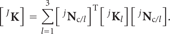
By writing the system potential energy, the system stiffness matrix [K] can be obtained as the summation of system link stiffness matrix $[{}^{L}K]$ and system joint stiffness matrix $[{}^{J}K]$ , both associated with the system total nodal coordinates {q}:

[K] = [{}^{L}K] + [{}^{J}K] .

(9)

In (6), the joint stiffness parameters will be set variable to match the variation of the system dynamic responses at different configurations. Therefore, (5), (8), and (9) are variable matrices.

Using static condensation method given by Guyan [12], the condensed system stiffness matrix [K_m] and mass matrix [M_m] are obtained as follows:

\begin{matrix} [K_{m}] & = {[N_{m}]}^{T} [K] [N_{m}] \\ - {[N_{m}]}^{T} [K] [N_{s}] {({[N_{s}]}^{T} [K] [N_{s}])}^{- 1} \\ \cdot {[N_{s}]}^{T} [K] [N_{m}], \end{matrix}

(10)

\begin{matrix} [M_{m}] & = {[N_{m}]}^{T} [M] [N_{m}] \\ - {[N_{m}]}^{T} [M] [N_{s}] {({[N_{s}]}^{T} [K] [N_{s}])}^{- 1} {[N_{s}]}^{T} [K] [N_{m}] \\ - {[N_{m}]}^{T} [K] [N_{s}] {({[N_{s}]}^{T} [K] [N_{s}])}^{- 1} {[N_{s}]}^{T} [M] [N_{m}] \\ + {[N_{m}]}^{T} [K] [N_{s}] {({[N_{s}]}^{T} [K] [N_{s}])}^{- 1} {[N_{s}]}^{T} [M] [N_{s}] \\ \cdot {({[N_{s}]}^{T} [K] [N_{s}])}^{- 1} {[N_{s}]}^{T} [K] [N_{m}], \end{matrix}

(11)

where [M] is system mass matrix, and [N_m] and [N_s] are partitioning matrices with elements of 1 and 0 which divide system total nodal coordinates {q} as master coordinatesg {q_m}, mainly consisted of the joint nodal coordinates, and slave coordinates {q_s} as follows:

{q} = [N_{m}] {q_{m}} + [N_{s}] {q_{s}} .

(12)

The above [K_m] and [M_m] are associated with the master coordinates {q_m}.

3. Eigen-Sensitivity on the Condensed System

According to Fox and Kapoor [13], the natural frequency sensitivity and mode shape sensitivity with respect to joint stiffness parameter $k_{b / l}$ , b = 1 to 7, l = 1 to 3, can be respectively, derived on the condensed system as

\begin{align} \frac{\partial f_{i}}{\partial k_{b / l}} & = \frac{1}{8 π^{2} f_{i}} {Φ_{i}}^{T} (\frac{\partial [K_{m}]}{\partial k_{b / l}} - ω_{i}^{2} \frac{\partial [M_{m}]}{\partial k_{b / l}}) {Φ_{i}}, \end{align}

(13)

\begin{matrix} \frac{\partial {Φ_{i}}}{\partial k_{b / l}} & = - \frac{1}{2} {Φ_{i}}^{T} \frac{\partial [M_{m}]}{\partial k_{b / l}} {Φ_{i}} {Φ_{i}} \\ + \sum_{\begin{matrix} j = 1 \\ j \neq i \end{matrix}}^{n} \frac{1}{ω_{i}^{2} - ω_{j}^{2}} {Φ_{i}}^{T} (\frac{\partial [K_{m}]}{\partial k_{b / l}} - ω_{i}^{2} \frac{\partial [M_{m}]}{\partial k_{b / l}}) \\ \cdot {Φ_{i}} {Φ_{j}}, \end{matrix}

(14)

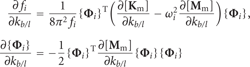
where f_i is the ith natural frequency, ${Φ_{i}}$ is the ith normalized mode shape vector, and $ω_{i} = 2 π f_{i}$ . Using (9) and noticing that $[{}^{L}K]$ and [M] are constant lead to

\begin{gathered} \frac{\partial [K]}{\partial k_{b / l}} = \frac{\partial [{}^{J}K]}{\partial k_{b / l}} \\ \frac{\partial [M]}{\partial k_{b / l}} = [0] . \end{gathered}

(15)

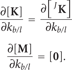
Therefore, the terms $\partial [K_{m}] / \partial k_{b / l}$ and $\partial [M_{m}] / \partial k_{b / l}$ in (13) and (14) can be calculated using (10) and (11) as

\begin{matrix} \frac{\partial [K_{m}]}{\partial k_{b / l}} \\ = {[N_{m}]}^{T} \frac{\partial [{}^{J}K]}{\partial k_{b / l}} [N_{m}] \\ - {[N_{m}]}^{T} \frac{\partial [{}^{J}K]}{\partial k_{b / l}} [N_{s}] {({[N_{s}]}^{T} [K] [N_{s}])}^{- 1} {[N_{s}]}^{T} [K] [N_{m}] \\ - {[N_{m}]}^{T} [K] [N_{s}] {({[N_{s}]}^{T} [K] [N_{s}])}^{- 1} {[N_{s}]}^{T} \frac{\partial [{}^{J}K]}{\partial k_{b / l}} [N_{m}] \\ + {[N_{m}]}^{T} [K] [N_{s}] {({[N_{s}]}^{T} [K] [N_{s}])}^{- 1} {[N_{s}]}^{T} \frac{\partial [{}^{J}K]}{\partial k_{b / l}} [N_{s}] \\ \cdot {({[N_{s}]}^{T} [K] [N_{s}])}^{- 1} {[N_{s}]}^{T} [K] [N_{m}], \end{matrix}

(16)

\begin{align} \frac{\partial [M_{m}]}{\partial k_{b / l}} \\ = {[N_{m}]}^{T} [M] [N_{s}] {({[N_{s}]}^{T} [K] [N_{s}])}^{- 1} {[N_{s}]}^{T} \frac{\partial [{}^{J}K]}{\partial k_{b / l}} [N_{s}] \\ \cdot {({[N_{s}]}^{T} [K] [N_{s}])}^{- 1} {[N_{s}]}^{T} [K] [N_{m}] \\ - {[N_{m}]}^{T} [M] [N_{s}] {({[N_{s}]}^{T} [K] [N_{s}])}^{- 1} {[N_{s}]}^{T} \frac{\partial [{}^{J}K]}{\partial k_{b / l}} [N_{m}] \\ + {[N_{m}]}^{T} [K] [N_{s}] {({[N_{s}]}^{T} [K] [N_{s}])}^{- 1} {[N_{s}]}^{T} \frac{\partial [{}^{J}K]}{\partial k_{b / l}} [N_{s}] \\ \cdot {({[N_{s}]}^{T} [K] [N_{s}])}^{- 1} {[N_{s}]}^{T} [M] [N_{m}] \\ - {[N_{m}]}^{T} \frac{\partial [{}^{J}K]}{\partial k_{b / l}} [N_{s}] {({[N_{s}]}^{T} [K] [N_{s}])}^{- 1} {[N_{s}]}^{T} [M] [N_{m}] \\ + {[N_{m}]}^{T} \frac{\partial [{}^{J}K]}{\partial k_{b / l}} [N_{s}] {({[N_{s}]}^{T} [K] [N_{s}])}^{- 1} {[N_{s}]}^{T} [M] [N_{s}] \\ \cdot {({[N_{s}]}^{T} [K] [N_{s}])}^{- 1} {[N_{s}]}^{T} [K] [N_{m}] \\ - {[N_{m}]}^{T} [K] [N_{s}] {({[N_{s}]}^{T} [K] [N_{s}])}^{- 1} {[N_{s}]}^{T} \frac{\partial [{}^{J}K]}{\partial k_{b / l}} \\ \cdot [N_{s}] {({[N_{s}]}^{T} [K] [N_{s}])}^{- 1} \\ \cdot {[N_{s}]}^{T} [M] [N_{s}] {({[N_{s}]}^{T} [K] [N_{s}])}^{- 1} {[N_{s}]}^{T} [K] [N_{m}] \\ + {[N_{m}]}^{T} [K] [N_{s}] {({[N_{s}]}^{T} [K] [N_{s}])}^{- 1} {[N_{s}]}^{T} [M] [N_{s}] \\ \cdot {({[N_{s}]}^{T} [K] [N_{s}])}^{- 1} {[N_{s}]}^{T} \frac{\partial [{}^{J}K]}{\partial k_{b / l}} [N_{m}] \\ - {[N_{m}]}^{T} [K] [N_{s}] {({[N_{s}]}^{T} [K] [N_{s}])}^{- 1} {[N_{s}]}^{T} [M] [N_{s}] \\ \cdot {({[N_{s}]}^{T} [K] [N_{s}])}^{- 1} \\ \cdot {[N_{s}]}^{T} \frac{\partial [{}^{J}K]}{\partial k_{b / l}} [N_{s}] {({[N_{s}]}^{T} [K] [N_{s}])}^{- 1} {[N_{s}]}^{T} [K] [N_{m}] . \end{align}

(17)

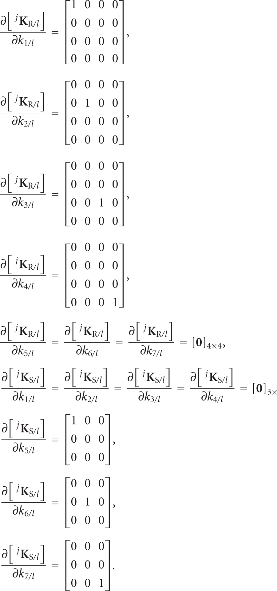
In light of (8), the term $\partial [{}^{J}K] / \partial k_{b / l}$ in (16) and (17) is

\begin{matrix} \frac{\partial [{}^{J}K]}{\partial k_{b / l}} & = \frac{\partial}{\partial k_{b / l}} \sum_{l = 1}^{3} {[{}^{j}{N_{c / l}}]}^{T} [{}^{j}{K_{l}}] [{}^{j}{N_{c / l}}] \\ \begin{matrix} = {[{}^{j}{N_{c / l}}]}^{T} \frac{\partial [{}^{j}{K_{l}}]}{\partial k_{b / l}} [{}^{j}{N_{c / l}}], b = 1 to 7; l = 1,2, 3, \end{matrix} \end{matrix}

(18)

where $\partial [{}^{j}{K_{l}}] / \partial k_{b / l}$ can be calculated using (5) as

\frac{\partial [{}^{j}{K_{l}}]}{\partial k_{b / l}} = [\begin{bmatrix} \frac{\partial [{}^{j}{K_{R / l}}]}{\partial k_{b / l}} & 0 & 0 \\ 0 & \frac{\partial [{}^{j}{K_{S / l}}]}{\partial k_{b / l}} & - \frac{\partial [{}^{j}{K_{S / l}}]}{\partial k_{b / l}} {[{}^{l}R]}^{T} [{}^{p}R] \\ 0 & ℭ & 픇 \end{bmatrix}],

(19)

where ℭ denotes $- {[{}^{p}R]}^{T} [{}^{l}R] (\partial [{}^{j}{K_{S / l}}] / \partial k_{b / l}),$ and 픇 denotes ${[{}^{p}R]}^{T} [{}^{l}R] (\partial [{}^{j}{K_{S / l}}] / \partial k_{b / l}) {[{}^{l}R]}^{T} [{}^{p}R]$ in which, by using (6) and (7), the differentials of the revolute and spherical joint stiffness matrices with respect to the joint stiffness parameters in the lth branch are

\begin{align} \frac{\partial [{}^{j}{K_{R / l}}]}{\partial k_{1 / l}} & = [\begin{bmatrix} 1 & 0 & 0 & 0 \\ 0 & 0 & 0 & 0 \\ 0 & 0 & 0 & 0 \\ 0 & 0 & 0 & 0 \end{bmatrix}], \\ \frac{\partial [{}^{j}{K_{R / l}}]}{\partial k_{2 / l}} & = [\begin{bmatrix} 0 & 0 & 0 & 0 \\ 0 & 1 & 0 & 0 \\ 0 & 0 & 0 & 0 \\ 0 & 0 & 0 & 0 \end{bmatrix}], \\ \frac{\partial [{}^{j}{K_{R / l}}]}{\partial k_{3 / l}} & = [\begin{bmatrix} 0 & 0 & 0 & 0 \\ 0 & 0 & 0 & 0 \\ 0 & 0 & 1 & 0 \\ 0 & 0 & 0 & 0 \end{bmatrix}], \\ \frac{\partial [{}^{j}{K_{R / l}}]}{\partial k_{4 / l}} & = [\begin{bmatrix} 0 & 0 & 0 & 0 \\ 0 & 0 & 0 & 0 \\ 0 & 0 & 0 & 0 \\ 0 & 0 & 0 & 1 \end{bmatrix}], \\ \frac{\partial [{}^{j}{K_{R / l}}]}{\partial k_{5 / l}} & = \frac{\partial [{}^{j}{K_{R / l}}]}{\partial k_{6 / l}} = \frac{\partial [{}^{j}{K_{R / l}}]}{\partial k_{7 / l}} = {[0]}_{4 \times 4}, \\ \frac{\partial [{}^{j}{K_{S / l}}]}{\partial k_{1 / l}} & = \frac{\partial [{}^{j}{K_{S / l}}]}{\partial k_{2 / l}} = \frac{\partial [{}^{j}{K_{S / l}}]}{\partial k_{3 / l}} = \frac{\partial [{}^{j}{K_{S / l}}]}{\partial k_{4 / l}} = {[0]}_{3 \times 3}, \\ \frac{\partial [{}^{j}{K_{S / l}}]}{\partial k_{5 / l}} & = [\begin{bmatrix} 1 & 0 & 0 \\ 0 & 0 & 0 \\ 0 & 0 & 0 \end{bmatrix}], \\ \frac{\partial [{}^{j}{K_{S / l}}]}{\partial k_{6 / l}} & = [\begin{bmatrix} 0 & 0 & 0 \\ 0 & 1 & 0 \\ 0 & 0 & 0 \end{bmatrix}], \\ \frac{\partial [{}^{j}{K_{S / l}}]}{\partial k_{7 / l}} & = [\begin{bmatrix} 0 & 0 & 0 \\ 0 & 0 & 0 \\ 0 & 0 & 1 \end{bmatrix}] . \end{align}

(20)

4. Modal Testing and Simulation

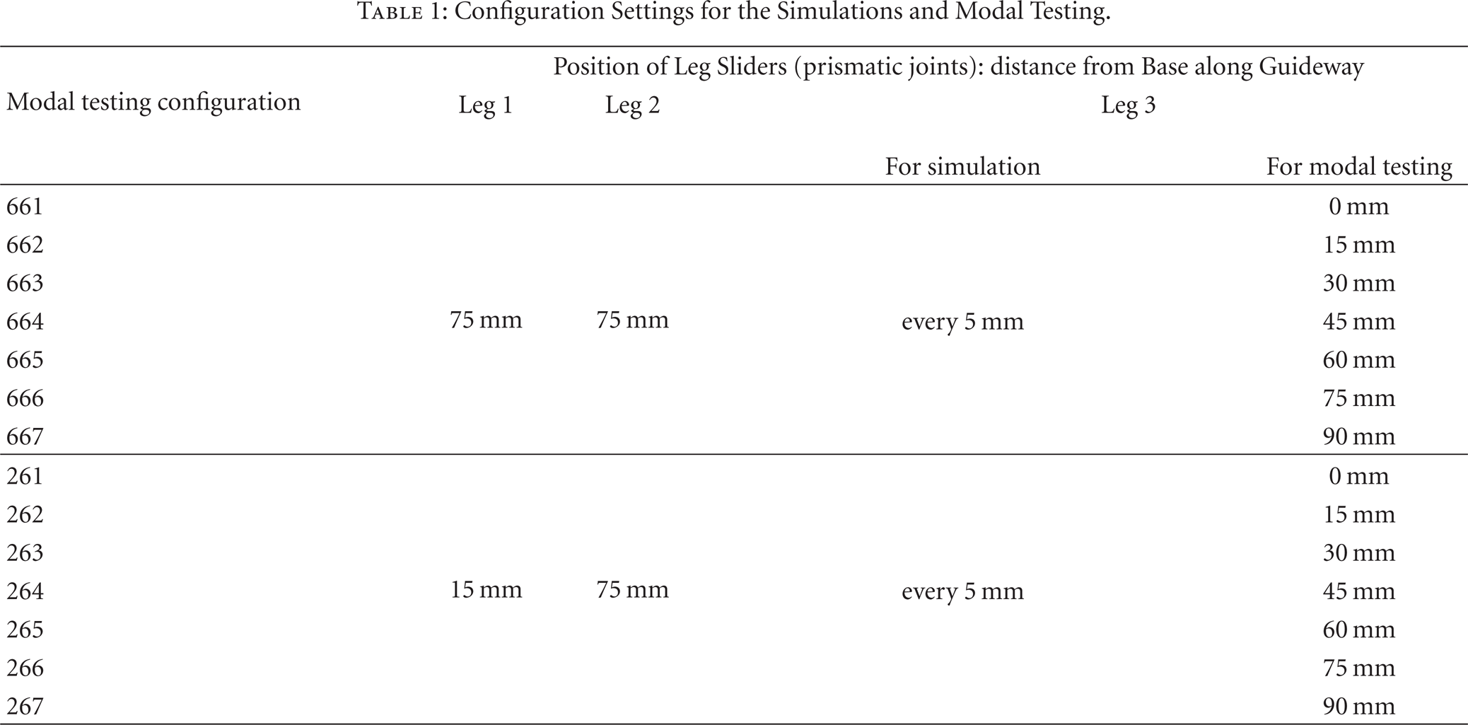
MATLAB codes were written based on the above analysis. The link model was built by using finite elements and was used to investigate the joint flexibility. For coordinate condensation, the selected master coordinates are the linear joint nodal coordinates in (4) in three branches (removing angular coordinate ${}^{l}{ϕ_{R}}$ due to the difficulty to measure), plus three linear nodal coordinates at the centre of the platform, where the cutting tool is supposed to be attached, along ^pX, ^pY, and ^pZ directions. Thus there are 30 master coordinates in total. All other coordinates are set slave. Table 1 shows the physical parameters of the robot. Table 2 lists the two sets of robot configurations that were used in the modal testing and simulation. They feature both asymmetric and symmetric robot configurations.

Table 1:

Configuration Settings for the Simulations and Modal Testing.

Modal testing configuration	Position of Leg Sliders (prismatic joints): distance from Base along Guideway
	Leg 1	Leg 2	Leg 3
			For simulation	For modal testing

661				0 mm
662				15 mm
663				30 mm
664	75 mm	75 mm	every 5 mm	45 mm
665				60 mm
666				75 mm
667				90 mm

261				0 mm
262				15 mm
263				30 mm
264	15 mm	75 mm	every 5 mm	45 mm
265				60 mm
266				75 mm
267				90 mm

Table 2:

Physical data for numerical calculations.

Length of leg	198	mm
Thickness of platform (modified)	18.5	mm
Triangle side length of platform (modified)	240	mm
Triangle side length of base bottom	270	mm
Length of guideway	90	mm
Slant angle of guideway from vertical	20	deg
Mass density of all parts	2710	kg/m³
Young's modulus of all parts	70	GN/m²
Poisson's ratio of all parts	0.33

Modal testing was conducted at each selected robot configuration. In order to understand the entire robot prototype, all measurement points were chosen to be evenly distributed on the platform and three legs. The excitation points were chosen close to the spherical joints on the moving platform. Accelerometers were used to detect the responses in the local body reference directions at the measurement points of each leg and the platform. The excitation and response signals were amplified and then recorded using LabVIEW where the FRF of each measurement is generated. The sampling frequency was 2000 Hz and sampling time was 1 second. The window function was set as force-exponential with 50% force window and 10% exponential window. The FRF measurements were imported to the postprocessing software ME'scope which extracts the system natural frequencies and operating deflection shapes (ODSs) that are theoretically close to the mode shapes.

With eigen-sensitivity (13) and (14) at hand, the natural frequencies and mode shapes in the model can be modified at the selected robot configurations according to the modal testing results by adjusting the joint stiffness parameters as follows:

{Δ k} = {[\begin{bmatrix} \frac{\partial f}{\partial k} \\ \frac{\partial Φ_{1}}{\partial k} \\ \frac{\partial Φ_{2}}{\partial k} \\ ⋮ \\ \frac{\partial Φ_{n}}{\partial k} \end{bmatrix}]}^{+} {\begin{Bmatrix} Δ f \\ Δ Φ_{1} \\ Δ Φ_{2} \\ ⋮ \\ Δ Φ_{n} \end{Bmatrix}},

(21)

where {Δk} represents the modification values of the 21 joint stiffness parameters; {Δf} represents the errors of natural frequencies between the measurement and the calculation; ${Δ Φ_{i}}$ , i = 1 to n, represents the errors of components in the ith mode shape between the measurement and the calculation; ∂f/∂k is the matrix whose elements are the values from (13); ∂Φ_i/∂k, i = 1 to n, is the matrix whose elements are the vector element values from (14); n is the eigen-solution order number; the superscript + stands for the Moore-Penrose pseudoinverse. Based on (21), an iteration procedure is formed to update the joint stiffness parameters until the errors of natural frequencies and mode shapes are within specified limits.

Figures 4(a), 4(b), and 4(c) show the stiffness parameters of the joint virtual springs for the robot configurations from 661 to 667, and Figures 5(a), 5(b), and 5(c) from 261 to 267 The initial joint stiffness parameters are uniformly set as 10⁵ N/m (or N*m/rad for k_4/l, l = 1, 2, 3) for all configurations. By using (21) for iteration, the joint stiffness parameters are obtained at the modal testing configurations 661 to 667 and 261 to 267, and linearly interpolated into the simulation configurations between these modal testing configurations. These figures indicate that the joint stiffness parameters are set configuration-dependent in order to match the variation of the system dynamic responses.

(a) Joint Stiffness in Branch 1 versus Configuration from 661 to 667. (b): Joint Stiffness in Branch 2 versus Configuration from 661 to 667. (c) Joint Stiffness in Branch 3 versus Configuration from 661 to 667.

(a) Joint Stiffness in Branch 1 versus Configuration from 261 to 267. (b) Joint Stiffness in Branch 2 versus Configuration from 261 to 267. (c) Joint Stiffness in Branch 3 versus Configuration from 261 to 267.

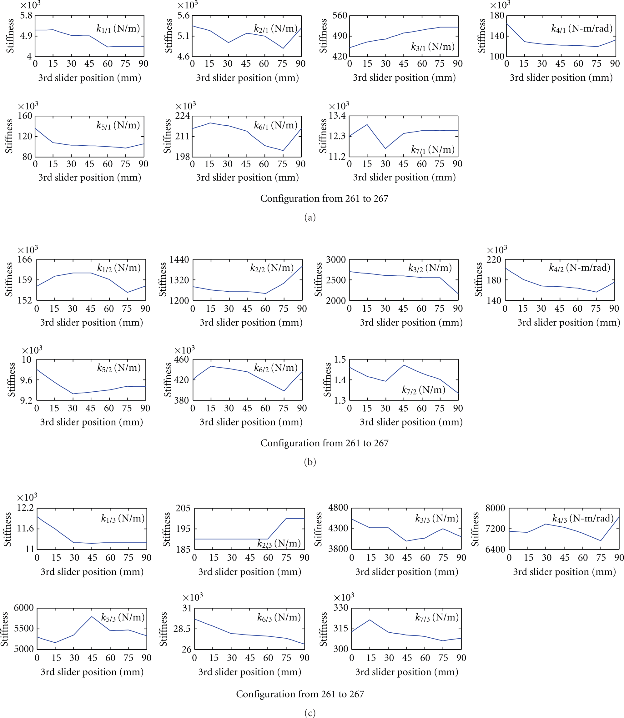
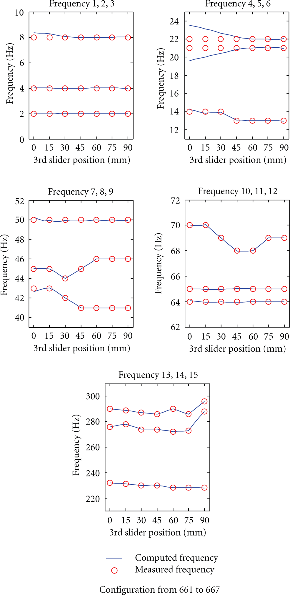
Figure 6 displays and compares the variations of the first 15 calculated and measured natural frequencies with the slider (prismatic joint) position changes starting at configuration 661 and ending at configuration 667 (referring to Table 1), and Figure 7 starting at configuration 261 and ending at configuration 267. The differences between the calculated and the measured frequencies are mostly less than 1%, and the largest deviations are less than 7% at the 5th and 6th natural frequencies at configurations 661 and 267. The possible reasons for the deviations are that the solutions of the joint stiffness parameters are locally optimal and that these two frequencies may be related with some slave coordinates.

Figure 6

Natural Frequency versus Configuration from 661 to 667.

Figure 7

Natural Frequency versus Configuration from 261 to 267.

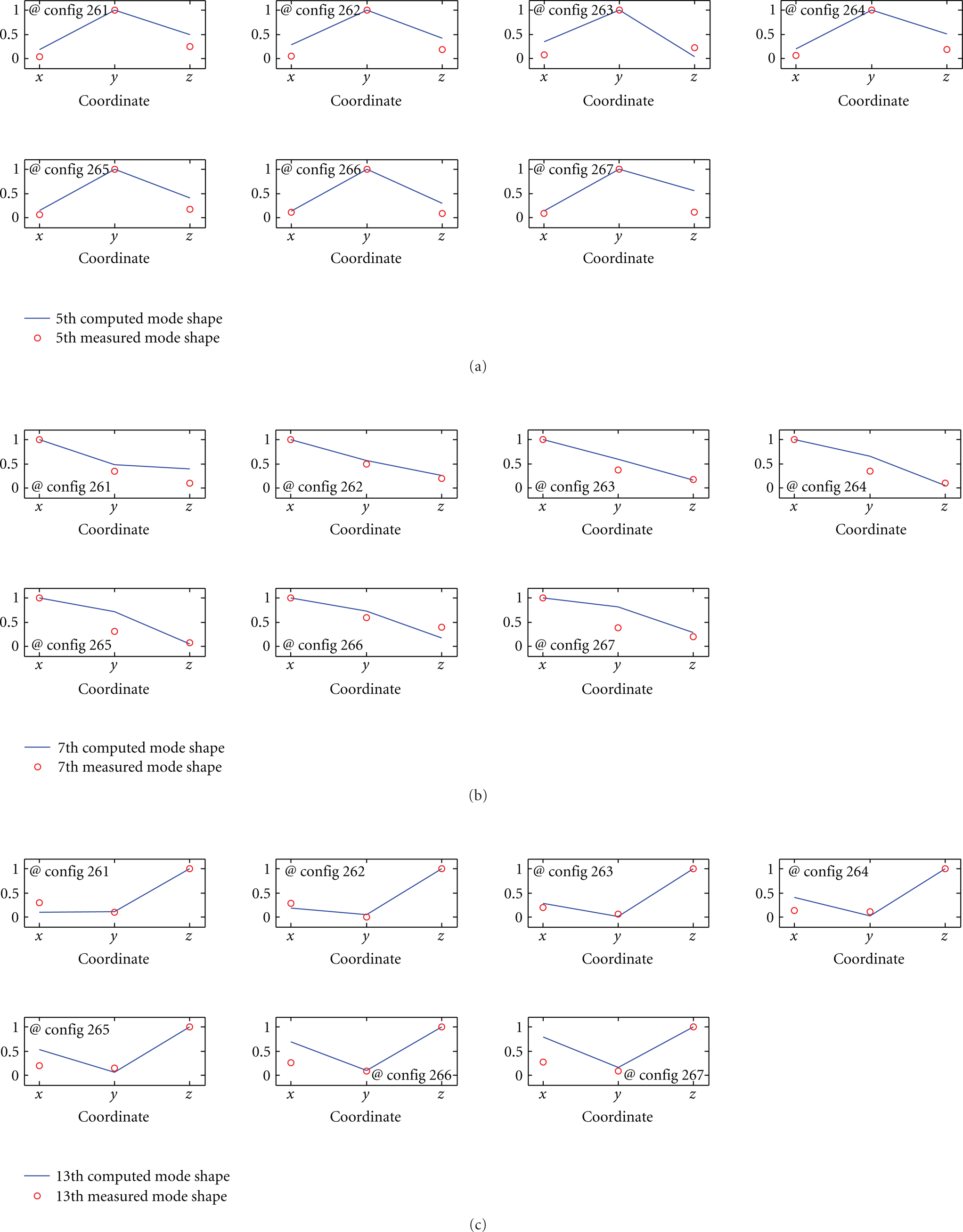
Figures 8(a), 8(b), and 8(c), respectively, display and compare the 5th, 7th, and 13th mode shapes at the node of the platform center (omitting mode shapes at other nodes) at configuration 661 to 667, and Figures 9(a), 9(b), and 9(c) at configuration 261 to 267 These mode shapes have the largest displacements at the platform center compared to other mode shapes: the 5th mode shape has the largest displacement in ^pY direction, the 7th in ^pX direction, and the 13th in ^pZ direction. For easy comparison, the selected mode shape components are normalized. These figures show that the calculated mode shapes are close to the measured ones although they do not perfectly agree. The disagreement may result from the undamped joint model on which the joint stiffness parameters are calculated. For the simplicity of the method, however, it is worthy of the small loss of mode shape accuracy.

(a) 5th Mode Shape at Platform Center at Configuration 661 to 667. (b) 7th Mode Shape at Platform Center at Configuration 661 to 667. (c) 13th Mode Shape at Platform Center at Configuration 661 to 667.

(a) 5th Mode Shape at Platform Center at Configuration 261 to 267. (b) 7th Mode Shape at Platform Center at Configuration 261 to 267. (c) 13th Mode Shape at Platform Center at Configuration 261 to 267.

It must be indicated that, for the ideal rigid (tight) joint model of the same robot, natural frequencies and mode shapes will also be variable with the configuration changing (not shown here), but the natural frequencies are much higher than those of the flexible joint model. In simulation of the ideal joint model, the first natural frequency is about 200 Hz and the second is about 500 Hz. Therefore, Figures 6–9 display the flexible joint effect on the system due to configuration changes.

5. Conclusions

This study presents a configuration-dependant flexible joint model for a parallel robot. The method is based on adaptation of virtual springs between the joint components to simulate the joint flexibility. The joint stiffness matrix of virtual springs was derived. The system was condensed at the joint nodal coordinates. Eigen-sensitivity analysis was conducted on the condensed system matrix with respect to the stiffness parameters of the joint virtual springs. Dynamic modification was conducted at a series of robot configurations for the virtual spring parameters to be set variable to match the variation of the system natural frequencies and mode shapes obtained from modal testing. The virtual spring parameters between the selected robot configurations were obtained by interpolation. The research indicates that the presented method is effective and relatively easy to conduct, compared to other methods. The variable flexible joint model is applicable to flexible multibody systems with variable configurations.

References

Tzou

H. S.

Rong

, and Nassirharand

, “Design and stochastic simulation of elastically jointed mechanical systems,” Computer-Aided Design, vol. 21, no. 7, pp. 435–440, 1989.

Bowden

and Dugundji

, “Joint damping and nonlinearity in dynamics of space structures,” American Institute of Aeronautics and Astronautics, vol. 28, no. 4, pp. 740–749, 1990.

Moon

F. C.

and Li

G. X.

, “Experimental study of chaotic vibrations in a pin-jointed space truss structure,” American Institute of Aeronautics and Astronautics, vol. 28, no. 5, pp. 915–921, 1990.

Tzou

H. S.

and Rong

, “Contact dynamics of a spherical joint and a jointed truss-cell system,” American Institute of Aeronautics and Astronautics, vol. 29, no. 1, pp. 81–88, 1991.

Kakizaki

Deck

J. F.

, and Dubowsky

, “Modeling the spatial dynamics of robotic manipulators with flexible links and joint clearances,” Journal of Mechanical Design, Transactions of the ASME, vol. 115, no. 4, pp. 839–847, 1993.

Seneviratne

L. D.

Earles

S. W. E.

, and Fenner

D. N.

, “Analysis of a four-bar mechanism with a radially compliant clearance joint,” Journal of Mechanical Engineering Science, vol. 210, no. 3, pp. 215–223, 1996.

Ravn

Shivaswamy

Alshaer

B. J.

, and Lankarani

H. M.

, “Joint clearances with lubricated long bearings in multibody mechanical systems,” Journal of Mechanical Design, Transactions of the ASME, vol. 122, no. 4, pp. 484–488, 2000.

Schwab

A. L.

Meijaard

J. P.

, and Meijers

, “A comparison of revolute joint clearance models in the dynamic analysis of rigid and elastic mechanical systems,” Mechanism and Machine Theory, vol. 37, no. 9, pp. 895–913, 2002.

Ting

K.-L.

Zhu

, and Watkins

, “Effects of joint clearance on position and orientation deviation of linkages and manipulators,” Mechanism and Machine Theory, vol. 35, no. 3, pp. 391–401, 2000.

10.

Zhu

and Ting

K.-L.

, “Uncertainty analysis of planar and spatial robots with joint clearances,” Mechanism and Machine Theory, vol. 35, no. 9, pp. 1239–1256, 2000.

11.

Wang

Gosselin

C. M.

, and Cheng

, “Modeling and simulation of robotic systems with closed kinematic chains using the virtual spring approach,” Multibody System Dynamics, vol. 7, no. 2, pp. 145–170, 2002.

12.

Guyan

R. J.

, “Reduction of stiffness and mass matrices,” American Institute of Aeronautics and Astronautics, vol. 3, no. 2, p. 380, 1965.

13.

Fox

R. L.

and Kapoor

M. P.

, “Rates of change of eigenvalues and eigenvectors,” American Institute of Aeronautics and Astronautics, vol. 6, no. 12, pp. 2426–2429, 1968.