Sage Journals: Discover world-class research

Abstract

The transportation mechanism of single solid particles in pulsating water flow in a vertical pipe was investigated by means of videography and numerical simulations. The trajectories of alumina particles were observed experimentally by stereo videography. The particle diameter was 3 mm or 5 mm, and the pipe diameter was 18 mm or 22 mm. The frequency of flow pulsation was less than or equal to 6.67 Hz. It was found that the critical minimum water flux at which the particle can be transported upward depended on the pulsating pattern. Two types of numerical simulations were conducted, namely, one-dimensional simulations for tracking the vertical motion of the solid particles and two-dimensional simulations of the pulsating pipe flows in an axisymmetric coordinate system. The computer simulations of axisymmetric pipe flows revealed that the time-averaged radial velocity profile of water in the pulsating flows was very different from that in steady pipe flows. The motion of the particles is discussed in detail for a better understanding of the physics of the transport phenomena.

1. Introduction

Air-lift pumps are used to vertically transport both liquid and small solid particles [1–8]. Figure 1 shows a schematic diagram of an air-lift pump used for transporting solid particles. It consists of a vertical lifting pipe and a gas injector. The buoyancy force of the injected gas induces an upward liquid flow in the pipe. The particles are lifted by the drag force generated by the surrounding liquid against the gravitational force. During the pump operation, the flow patterns above the gas injector show slug or churn-turbulent flows depending on the injected gas flow rate. In the slug flow regime, liquid and gas slugs appear alternately along the pipe, resulting in a periodic flow motion. In the churn-turbulent flow regime, the flows fluctuate and are chaotic. Regardless of the flow patterns, the motion of the particles is complex because of the unsteady motion of the surrounding fluid.

Figure 1

Schematic diagram of an air-lift pump for conveying solid particles.

In the region below the gas injector where the liquid and the solid particles are present, the flows are unsteady as well. The local liquid velocity below the gas injector is a rate-controlling parameter for the transportation of solid particles [1–3]. Understanding the flow structure in the two-phase region is thus important for developing a model capable of predicting the pumping characteristics. There have been prior studies of air-lift pumps [1–7], as reviewed in a later subsection, but the details of the unsteady flow motion in the two-phase region remain unclear. The understanding of the transport mechanism of solid particles is limited and thus this mechanism is investigated in the present study.

The critical minimum water flux at which a single solid particle can be lifted vertically upward is one of the key parameters in designing air-lift systems for transporting solid particles. In prior works [1–3], the critical flux has been discussed in terms of the mean liquid flux, the properties of the solid material, and the particle size. The effect of the unsteady liquid motion was ignored; it is examined in the present study.

Particle-liquid two-phase flows arise not only in air-lift pumps, but also in other industrial applications. There have been many studies of pulsating liquid flow in such applications, although the flow conditions differ from those in air-lift pumps. This work will be reviewed in a later subsection.

In the present study, the transport characteristics of single solid particles in pulsating liquid pipe flows were investigated by carrying out experiments and numerical simulations as basic research on air-lift pumps in the slug flow regime. In the experiments, the three-dimensional unsteady particle motion was observed by stereo videography. The internal pipe diameter was 18 mm or 22 mm, and water was used as the test liquid at room temperature. The diameter of the spherical alumina solid particles was 3 mm or 5 mm. The frequency of the flow pulsation ranged from 3.33 Hz to 6.67 Hz. It was found that the critical minimum liquid flux at which a particle can be lifted upward depended on the pulsation pattern.

Two types of numerical simulations were conducted: simulations for tracking the particle trajectory in a one-dimensional coordinate system, and computations of the pulsating flows in the pipe in an axisymmetric coordinate system. The particle motion is discussed in detail for a better understanding of the transport phenomena.

2. Literature Survey

Several researchers have studied air-lift pumps for lifting solid particles. Weber and Dedegil [6] conducted experiments using a large-scale air-lift pump, the length of which ranged from 50 to 441 m with a diameter of 300 mm. They used three kinds of solid particles and measured the volume of the discharged particles for different gas injection points. Hatta et al. [4], Kato et al. [5], and Yoshinaga and Sato [7] carried out experiments using relatively small air-lift pumps for conveying solid particles. They aimed to validate their theoretical models for predicting pump performance, namely the relationship between the volumetric fluxes of supplied air and discharged particles or the relationship between the volumetric fluxes of supplied air and discharged liquid. The total pipe length was less than 10 m in their experiments. Fujimoto et al. [1–3] investigated pump performance using a small air-lift system. In these studies, the main goal was to find or to predict the pump performance. The unsteady flow motion in the two-phase region below the gas injector received little attention.

Pulsating pipe flows have been studied not only because of their industrial applications, but also because of their fundamental significance for scientific research. We first review studies of single-phase pulsating pipe flows. Early studies of turbulent pulsating pipe flows were reported by Ramaprian and Tu [9–11]. They used a single-component laser-Doppler-anemometry system to measure the local instantaneous velocity in a pipe with an internal diameter of 50 mm and a Reynolds number of 50000. Shemer et al. [12] measured the velocity distribution and turbulent shear stress using a hot-wire anemometer over a wide range of mean-flow Reynolds numbers. Hwang and Brereton [13] and Brereton and Mankbadi [14] investigated turbulent pulsating pipe flows. Eguchi et al. [15] measured the velocity distribution of pulsatile flows in a vertical rigid and elastic tube using a PIV measurement technique. Ünsal and Durst [16] studied both fully developed steady pipe flows and pulsating flows with the Reynolds number ranging from 180 to 18000 and a pipe diameter of 15 mm. He and Jackson [17] investigated pulsating turbulent flows in a pipe using a two-component laser Doppler anemometer (LDA). He et al. [18] calculated accelerating pipe flows with a low-Reynolds-number k-ε turbulence model. Blel et al. [19] experimentally studied the shear stress of turbulent pulsatile flows.

Several researchers have investigated pulsating liquid flows containing solid particles. Akhremenko et al. [20] theoretically studied the dynamics of the motion of solid particles in fluid flows with a flow-rate pulsation frequency of up to 1 Hz. Suzuki et al. [21] carried out computer simulations of the unsteady motion of small particles in a square chamber with a pulsating inlet velocity. Carvalho Jr. [22] computed the characteristics of solid particles in the pulsating gas flow of a Rijke-type combustor using a fourth-order Runge-Kutta scheme. Saito et al. [23] examined the characteristics of particle velocity in the main stream direction of solid-liquid two-phase flows in a swaying pipe. They derived the equation of motion for solid particles in the swaying pipe by considering the virtual mass, the Basset term, and the frictional force between the particles and the pipe wall. Eesa and Barigou [24] numerically investigated the laminar pipe transport of coarse particles in non-Newtonian fluid. El Masry and El Shobaky [25] experimentally studied the pulsating turbulent flow of sand-water suspension in a tube of diameter 3.3 cm under the conditions that the frequency was 0.1–1.0 Hz and the mean Reynolds number was 33000–82000.

Particle-liquid two-phase flow in a pipe is affected by many parameters including pipe diameter, particle size, liquid and solid materials, mean flow rates, and pulsating frequency. Unlike steady single-phase pipe flow, pulsating flow and its particle motion cannot be correlated using a few dimensionless parameters. The present experiments were carried out under different conditions from those used in previous studies.

3. Setup

3.1. Experimental Apparatus

Figure 2(a) shows a schematic diagram of the experimental apparatus. The total length of the vertical lifting pipe made of transparent plastic is 2870 mm and its inner diameter is 18 or 22 mm. Water at room temperature (15°C or 20°C) was used as the test liquid. Water is supplied at the bottom of the lifting pipe through an inflow unit, flows upward in the pipe, and is discharged at the top, which is open to the atmosphere. Discharged water from the top of the riser pipe returns to the reservoir.

Schematic diagram of experimental apparatus.

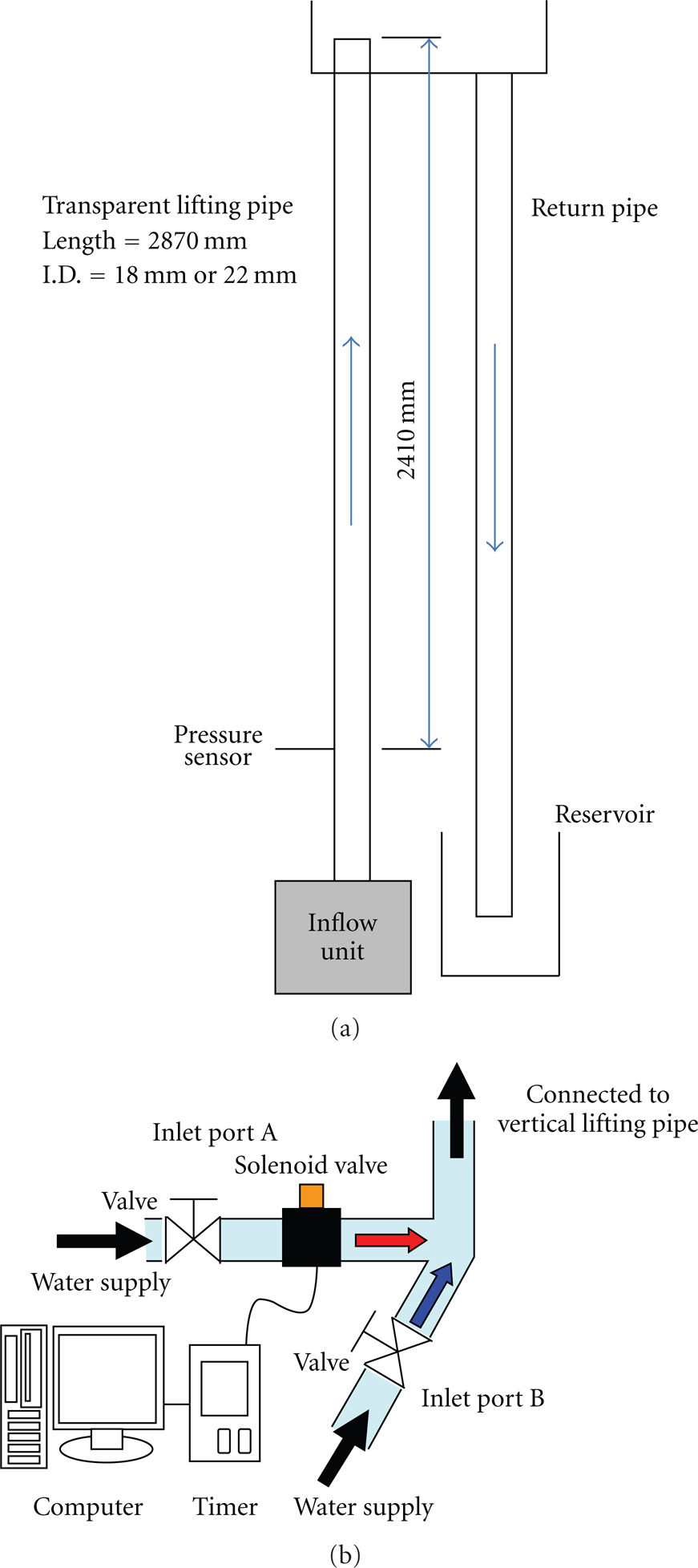
Figure 2(b) shows the schematics of the inflow unit, consisting of two inlet ports A and B. An electromagnetic valve was attached at port A to make pulsating flows. When the electromagnetic valve was open, water could be supplied into the lifting pipe from both ports. When the valve was closed, water was supplied only from port B. The operation of the electromagnetic valve was controlled by a digital timer. The periods of the valve opening, t_on, and the valve closing, t_off, could be arbitrarily determined by the delay timer with a time resolution of 10 ms. It should be noted that an additional response time (at most 5 ms) is needed to mechanically activate or deactivate the electromagnetic valve. The following two parameters were introduced to describe the following pulsation patterns:

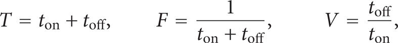
T = t_{on} + t_{off}, F = \frac{1}{t_{on} + t_{off}}, V = \frac{t_{off}}{t_{on}},

(1)

where T and F are the period and frequency of the flow pulsation. The parameter V becomes zero in the case of steady pipe flow. The pulsating frequencies tested in this study were 3.33, 5.55, and 6.67 Hz and V ranged from 0.15 to 1.0. The minimum period of the valve closing, t_off, was 40 ms, taking into account the time resolution of the delay timer (=10 ms) as well as the response time of the electromagnetic valve (∼5 ms).

The pressure sensor was attached 2410 mm from the top of the lifting pipe (see Figure 2(a)). A digital data recorder was used to measure the transient hydrostatic pressure relative to the atmospheric pressure with a sampling time of 1 ms. The timings of the valve activations were also recorded.

Spheres made of alumina with a material density of 3600 kg/m³ were used as the solid particles. The particle diameter d was 3 mm or 5 mm. The mean volume flow rate of water, Q_L, was determined by the volume of discharged water and a sampling time of 30 s, which was sufficiently long compared to the maximum pulsating period, T (=0.3 s). The mean water flux j_L was determined by the volume flow rate of water Q_L and the cross-sectional area A of the lifting pipe as follows:

j_{L} = \frac{Q_{L}}{A} .

(2)

It is noted that the measurement accuracy of j_L is within ±0.005 m/s. A preset constant volume flow rate, Q_LC, of water from the inlet port without the electromagnetic valve was also measured. The flux of the constant flow, j_LC, was determined as

j_{L C} = \frac{Q_{L C}}{A} .

(3)

In addition, the ratio of the constant volume flow rate to the total volume flow rate, C_ratio, was defined by

C_{ratio} = \frac{Q_{L C}}{Q_{L}} .

(4)

The value of C_ratio is between 0 and 1. The flow is steady when C_ratio = 1. The conditions of the flow pulsations are specified by the four parameters, F,V,C_ratio, and j_L.

3.2. Videography and Data Reduction for Particle Motion

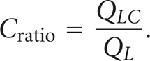
To gain an understanding of the unsteady motion of the particles in the lifting pipe, videographic observation was conducted. Figure 3 depicts a schematic diagram of the videography and the definition of the coordinates. The origin is set 2130 mm from the top of the lifting pipe in the center axis. The z-axis is set in the vertically upward direction from the origin. The x- and y-axes are set in the horizontal plane.

Figure 3

Schematic diagram of stereo videography and definition of coordinate system.

A square duct with a cross section of 40 × 40 mm² was coaxially set to the lifting pipe in the observation section. The space between the inner wall of the square duct and the outer wall of the pipe was filled with water to minimize the refraction and reflection of light at the curved outer wall of the pipe. Two digital video cameras were placed at z = 730 mm. The two optical axes of the video cameras were set along the x- and y-axes as defined in the figure so that the spatial position of the particles in the pipe could be identified correctly. Video images were taken every 1/30 s with a resolution of 1920 × 1080 pixels.

The trajectory of the particles in the lifting pipe was directly measured from the video images. The measurement uncertainties of the coordinates were within ±0.3 mm. The particle velocity was determined from the distance moved between two successive video images and the frame rate (=30 s⁻¹). If a particle located at (x, y, z) = (x_n, y_n, z_n) in a video frame moves to (x, y, z) = (x_n+1, y_n+1, z_n+1) in the subsequent frame, the particle velocity ( ${\dot{x}}_{n}, {\dot{y}}_{n}, {\dot{z}}_{n}$ ) is evaluated as

{\dot{x}}_{n} = \frac{x_{n + 1} - x_{n}}{30}, {\dot{y}}_{n} = \frac{y_{n + 1} - y_{n}}{30}, {\dot{z}}_{n} = \frac{z_{n + 1} - z_{n}}{30} .

(5)

The particle positions are also represented in the cylindrical coordinate system as (r, θ, z) = (r_n, θ_n, z_n) in the radial coordinate, the azimuthal angle, and the vertical coordinate. They were evaluated via the following:

r_{n} = \sqrt{x_{n}^{2} + y_{n}^{2}}, θ_{n} = ta n^{- 1} \frac{y_{n}}{x_{n}} .

(6)

4. Numerical Procedure

Two types of numerical simulations were conducted. The first was a one-dimensional simulation to track the particle trajectories in the z-direction in the pulsating liquid flows. The second was used to calculate the axisymmetric pulsating pipe flows. The numerical procedures are explained below.

4.1. One-Dimensional Simulation of Particle Motion

The one-dimensional momentum equation for a single particle in a liquid, taking account of the gravity, the drag force between the particle and the surrounding fluid, and the virtual mass force, is

\begin{matrix} \frac{4}{3} π {(\frac{d}{2})}^{3} ρ_{p} \frac{D v_{p}}{D t} & = \frac{4}{3} π {(\frac{d}{2})}^{3} (ρ - ρ_{p}) g \\ + C_{D} \frac{1}{2} ρ (v - v_{p}) | v - v_{p} | π {(\frac{d}{2})}^{2} \\ + \frac{1}{2} ρ \frac{4}{3} π {(\frac{d}{2})}^{3} \frac{D}{D t} (v - v_{p}), \end{matrix}

(7)

where t, ρ, ρ_p, v, v_p, d, C_D, and g are the time, the densities of the liquid and solid, the axial upward velocities of the liquid and solid phases, the particle diameter, the drag coefficient, and the gravitational acceleration, respectively. Then, we have the following equation:

\begin{matrix} ρ_{p} \frac{D v_{p}}{D t} & = (ρ - ρ_{p}) g + \frac{3 ρ C_{D}}{4 d} (v - v_{p}) | v - v_{p} | \\ + \frac{ρ}{2} \frac{D}{D t} (v - v_{p}) . \end{matrix}

(8)

The particle motion governed by (8) was numerically solved by the fourth-order Runge-Kutta method with a sufficiently small time increment under the conditions that the initial particle velocity is zero and the liquid velocity is assumed to obey the following semistep function of time:

v_{l} = {\begin{cases} j_{L} [C_{ratio} + \frac{1}{2} (1 + V) (1 - C_{ratio}) {1 - \cos (\frac{π \cdot t_{e}}{δ})}] \\ (0 \leq t_{e} < δ), \\ j_{L} [C_{ratio} + (1 + V) (1 - C_{ratio})] \\ (δ \leq t_{e} < t_{on}), \\ j_{L} [C_{ratio} + \frac{1}{2} (1 + V) (1 - C_{ratio}) \\ \times {1 - \cos (π (1 + \frac{t_{e} - t_{o n}}{δ}))}] \\ (t_{on} \leq t_{e} < t_{on} + δ), \\ j_{L} C_{ratio} (t_{on} + δ \leq t_{e} < T), \end{cases}

(9)

where t_e is the elapsed time after an activation of the electromagnetic valve in inlet port A. The above velocity profile is given by a continuous function introducing a small transient time δ (=10 ms) to avoid unexpected numerical errors due to abrupt changes in the velocity.

The drag coefficient C_D is evaluated as a function of the particle Reynolds number, Re_p [26] as follows:

C_{D} = {\begin{cases} \frac{24}{R e_{p}} (1 + 0.15 R e_{p}^{0.687}) \\ R e_{p} (= \frac{ρ | v_{l} - v_{p} | d}{μ}) \leq 700, \\ {\sqrt{\frac{24}{R e_{p}}} + 0.34 (R e_{p}^{0.06} + \frac{1}{1.72 + 0.018 R e_{p}})}^{2} \\ R e_{p} > 700, \end{cases}

(10)

where μ is the liquid viscosity. In addition, the particle position z_p is calculated as

z_{p} = z_{0} + \int v_{p} d t,

(11)

where z₀ is the initial particle position (z₀ = 0).

4.2. Two-Dimensional Simulation for Analyzing Liquid Pipe Flows

The pulsating pipe flows were assumed to obey the continuity and Navier-Stokes equations for incompressible fluids in the axisymmetric coordinate system as follows:

\begin{align} \begin{matrix} \frac{1}{r} \frac{\partial (r u)}{\partial r} + \frac{\partial v}{\partial z} = 0, \end{matrix} \end{align}

(12)

\begin{matrix} \frac{\partial u}{\partial t} + u \frac{\partial u}{\partial r} + v \frac{\partial u}{\partial z} \\ = - \frac{1}{ρ} \frac{\partial p}{\partial r} + \frac{μ}{ρ} (\frac{1}{r} \frac{\partial^{2} (r u)}{\partial r^{2}} - \frac{u}{r^{2}} + \frac{\partial^{2} u}{\partial z^{2}}), \end{matrix}

(13)

\begin{matrix} \frac{\partial v}{\partial t} + u \frac{\partial v}{\partial r} + v \frac{\partial v}{\partial z} \\ = - \frac{1}{ρ} \frac{\partial p}{\partial z} + \frac{μ}{ρ} (\frac{1}{r} \frac{\partial^{2} (r v)}{\partial r^{2}} + \frac{\partial^{2} v}{\partial z^{2}}) - g, \end{matrix}

(14)

where (u,v),p, and g are the velocity components in the radial and axial directions, the pressure, and the gravitational acceleration. No turbulence model was included in the present study, although this would make our model more realistic.

The conservation equations were approximated and solved by the CIP (cubic-interpolated pseudoparticle) method [27]. The Navier-Stokes equation (13) was split into three stages:

\begin{gathered} \frac{\overset{\circ}{u} - u^{n}}{Δ t} + u \frac{\partial u}{\partial r} + v \frac{\partial u}{\partial r} = 0, \end{gathered}

(15)

\begin{matrix} \frac{\tilde{u} - \overset{\circ}{u}}{Δ t} = \frac{μ}{ρ} (\frac{1}{r} \frac{\partial^{2} (r u)}{\partial r^{2}} - \frac{u}{r^{2}} + \frac{\partial^{2} u}{\partial z^{2}}), \end{matrix}

(16)

\begin{gathered} \frac{u^{n + 1} - \tilde{u}}{Δ t} = - \frac{1}{ρ} \frac{\partial p}{\partial r}, \end{gathered}

(17)

where Δt, $\overset{}{u}$ , and $\tilde{u}$ represent the time increment and the first and second intermediate velocities. The superscript n denotes the time step. Similarly, (14) is divided into three equations. Equation (15) is solved by the CIP scheme to obtain $\overset{}{u}$ . Then, the second intermediate velocity $\tilde{u}$ is calculated. The central difference scheme was used for the viscous terms in (16). The pressure profile was calculated by the following Poisson equation:

\frac{1}{r} \frac{\partial}{\partial r} (r \frac{\partial p}{\partial r}) + \frac{\partial^{2} p}{\partial z^{2}} = \frac{ρ}{Δ t} (\frac{1}{r} \frac{\partial (r \tilde{u})}{\partial r} + \frac{\partial \tilde{v}}{\partial z}),

(18)

where $\tilde{v}$ is the second intermediate velocity in the z-direction.

Figure 4 shows a schematic of the computational domain, which was divided into 800 meshes in the vertical direction and 40 meshes in the radial direction. Initially, the pipe was filled with quiescent water. Flow pulsation started at time t = 0 s. The inflow conditions were imposed at the inflow boundary (A). The inflow velocity v_l was given by (9), which is dependent on the time but independent of the radial coordinate. The no-slip conditions (u = v = 0) were employed at the wall boundary (B). The symmetric conditions were used at the center axis (C). At the outflow boundary (D), the zero velocity-gradient conditions were applied and the pressure is equal to the atmospheric pressure.

Figure 4

Schematic diagram of computational domain for calculating liquid flow.

Since the initial velocity of the liquid is zero, the calculated velocity profile shows nonperiodic motion in the early stages. According to preliminary numerical simulations, the velocity profile becomes almost periodic when t > 3 s. Therefore, the numerical results will be given for t > 3 s.

5. Results and Discussion

5.1. Videographic Observation of Particle Motion in Steady Pipe Flows

The motion of the particles in steady pipe flows was observed by means of the aforementioned method to clarify the differences between steady and pulsating flows. Figure 5(a) shows the trajectory of an alumina particle in the vertical (r-z) plane plotted every 1/30 s for j_L = 0.530 m/s, d = 5 mm, and D = 22 mm. The water temperature was 20°C. Consecutive points showing the center positions of the particle are connected with dotted line segments. The particle travels upward along the pipe wall (at r ∼ 8 mm) at an almost constant velocity. Because the particle radius is 2.5 mm, the actual distance between the pipe wall and the outer side of the particle surface is very small. Figure 5(b) shows the time variation of the vertical position of the particle. The upward velocity of the particle varies slightly with time. Figure 5(c) shows an overhead view of the particle trajectory in the x-y plane. The particle is always present near the wall surface, and it has a small velocity component in the circumferential direction.

Motion of alumina particle in steady upward flow for d = 5 mm, D = 22 mm, and j_L = 0.530 m/s.

To examine the particle motion in steady pipe flows from a stochastic viewpoint, the radial positions of particles passing at z = 730 mm were measured 100 times under conditions the same as those in Figure 5. As shown in Figure 6, the particles always exist close to the pipe wall and their positions are independent of the circumferential direction.

Figure 6

Radial positions of particles passing at z = 680 mm for d = 5 mm, D = 22 mm, and j_L = 0.530 m/s.

In fully developed pipe flows, the vertical liquid velocity is large at the center axis, decreases radially outward, and is zero at the wall, as shown in Figure 7. Let us consider the case where the particle is located near the pipe wall at almost zero velocity. At the surface of the solid particle, the liquid velocity becomes almost zero and the pressure increases. The pressure at the solid surface in the inner region (red region) is larger than that in the outer region (yellow region) in the figure because of the liquid velocity profile, so the surrounding liquid exerts a radially outward drag force on the particles. As a consequence, the particles are pushed radially outward and are located near the pipe wall. It should be noted that similar results were obtained in experiments carried out by varying the pipe diameter and particle size.

Figure 7

Schematic of liquid velocity profile and drag force acting on particle.

The critical minimum water flux at which a single solid particle can be lifted vertically upward is one of the key parameters in designing air-lift systems used for transporting solid particles. The critical flux was measured in the following manner. Initially, the liquid was at rest in the riser pipe. The water flow rate was then increased slowly by adjusting the regulating valve. When it exceeded a certain value, the particle started to move upward and the critical flux could be determined. Table 1 shows the critical minimum water fluxes, j_{L min, steady}, for steady pipe flows when the water temperature was 20°C and the internal pipe diameter was 22 mm. We tested both alumina particles and glass particles with a 3-mm diameter and a material density of 2520 kg/m³. The critical water fluxes depend on the material density of the solid and the particle diameter. They increase with increasing material density or increasing particle size.

Table 1:

Critical minimum water flux for lifting single particles in steady pipe flows and terminal velocity.

Material, particle diameter	Critical water flux, j_{L min, steady}	The terminal velocity of particles in quiescent water

Alumina, 5mm	0.520 m/s	0.418 m/s
Alumina, 3 mm	0.460 m/s	0.400 m/s
Glass, 5 mm	0.405 m/s	0.333 m/s

The results can be explained by (8). Assuming Dv_p/Dt, v_p = 0, and the uniform radial velocity profile of liquid in the pipe, we have the following liquid velocity corresponding to the critical water fluxes, j_{L min, steady},

j_{l \min, steady} = \sqrt{\frac{4 d g (ρ_{p} - ρ_{l})}{3 ρ_{l} C_{D}}} .

(19)

It is apparent from (19) that a higher liquid velocity is needed to lift particles with larger material density or larger diameter. The experimental results listed in Table 1 are consistent with this equation.

The terminal velocity of a solid particle descending in quiescent water in the vertical pipe was also measured for comparison; see Table 1. The terminal velocity is appreciably smaller than the critical minimum flux in all cases and the particles descended near the center axis. In contrast, the particles in the upward steady pipe flows were located near the pipe wall where the liquid velocity is small. As a consequence, the critical flux was larger than the terminal velocity.

5.2. Videographic Observation of Particle Motion in Pulsatile Pipe Flows

Figure 8 shows the typical motion of an alumina particle in a pulsating upward flow. The pulsation pattern was F = 6.67 Hz, C_ratio = 0.0, and V = 0.5. The water flux, the particle diameter, and the pipe diameter were j_L = 0.39 m/s, d = 5 mm, and D = 22 mm. The water temperature was 20°C. In contrast to the steady flows, the particle moves both vertically and radially. It shows up-and-down motion and the water pressure relative to the atmospheric pressure varies periodically with time. Since the particle velocity becomes temporarily negative, the total distance moved by the lifted particle is much longer than the length of the riser pipe. The particle often passes near the center axis.

Time histories of (a), (b), and (d) positions of alumina particle and (c) pressure in pulsating upward flow where F = 6.67 Hz, C_ratio = 0.0, V = 0.5, j_L = 0.39 m/s, d = 5 mm, and D = 22 mm.

Figure 9 shows the particle trajectories in the horizontal plane for various conditions. The experimental conditions are listed in Table 2. In all cases, C_ratio was zero and the water temperature was 20°C. In contrast to the steady flows, the particles move both near the pipe wall and in the center axis. The chance of particles being near the center axis depends on the pulsation pattern.

Table 2:

List of experimental conditions in Figure 9.

Case	Frequency, F	V	C _ratio	Mean water flux, j_L	Pipe diameter, D	Particle diameter, d

a	3.33 Hz	0.5	0.0	0.470 m/s	22 mm	5 mm
b	3.33 Hz	1.0	0.0	0.470 m/s	22 mm	5 mm
c	3.33 Hz	0.5	0.0	0.395 m/s	18 mm	3 mm
d	6.67 Hz	0.5	0.0	0.365 m/s	18 mm	3 mm

Particle trajectories in horizontal plane for (F,V,j_L,D,d) = (a) (3.33 Hz, 0.5, 0.470 m/s, 22 mm, 5 mm), (b) (3.33 Hz, 1.0, 0.470 m/s, 22 mm, 5 mm), (c) (3.33 Hz, 0.5, 0.395 m/s, 18 mm, 3 mm), and (d) (6.67 Hz, 0.5, 0.365 m/s, 18 mm, 3 mm).

The detailed radial motion of the particles was observed by high-speed videography with a frame rate of 300 s⁻¹ and a resolution of 512 × 384 pixels. Figure 10 shows the time variation of the radial particle position under the conditions of Figure 9(d). The positions of r = 0.0 mm and 7.5 mm coincide with the center axis and the pipe wall, respectively. It can be seen that the particle tends to move radially inward during the valve closing, suggesting that the radially inward force acts on the particle in the aftermath of the valve closure. Although the figure shows only five pulsation cycles, similar particle motion was frequently observed when the particles were located near the pipe wall. Further discussion will be given in a later subsection, using the results of the two-dimensional simulation for pulsating pipe flows.

Figure 10

Time variation of radial particle position for F = 6.67 Hz, V = 0.5,C_ratio = 0.0, and j_L = 0.365 m/s.

The effect of C_ratio on the particle motion is now investigated. Figure 11 shows the typical particle motion for F = 3.33 Hz, V = 0.5, C_ratio = 0.20, and j_L = 0.505 m/s. The results for F = 3.33 Hz, V = 0.5, C_ratio = 0.96, and j_L = 0.520 m/s are shown in Figure 12. In both cases, the diameter of the alumina particles is d = 5 mm, the pipe diameter is D = 22 mm, and the temperature of the water is 20°C. It should be noted that the water fluxes in the two results are not the same, but are comparable. The particle in Figure 11 has up-down motion. In contrast, the particle in Figure 12 always moves upward since the velocity change is small for a larger C_ratio. The particle moves upward along the pipe wall in a motion similar to that observed for the steady flows.

Figure 11

Particle motion for F = 3.33 Hz, V = 0.5, C_ratio = 0.20, and j_L = 0.505 m/s.

Figure 12

Particle motion for F = 3.33 Hz, V = 0.5, C_ratio = 0.96, and j_L = 0.520 m/s.

In the present study, the lifting pipes with internal diameters of D = 18 and 22 mm were expected to affect the unsteady particle motion. However, we did not observe any appreciable effects of the pipe diameter on the particle motion.

5.3. One-Dimensional Simulation for Tracking Particle Trajectory

Figure 13 shows the time evolution of the predicted particle velocity in the z-direction for (F, V, C_ratio, j_L) = (a) (3.33 Hz, 0.5, 0.0, 0.64 m/s), (b) (4.16 Hz, 0.5, 0.0, 0.64 m/s), (c) (6.67 Hz, 0.5, 0.0, 0.64 m/s), and (d) (4.16 Hz, 0.5, 0.56, 0.64 m/s). The measured particle velocities are also plotted in the figure to validate the numerical model. As expected, the predicted particle motion is up-and-down according to the flow pulsation. For the cases of C_ratio = 0.0 ((a) to (c)), the predicted particle velocities are in fairly good agreement with the experiments, although the one-dimensional model using (8) is ideal as compared to the actual flows. In (d), the discrepancy between the predictions and the experiments is appreciable. We carried out the simulations under various flow conditions and found that the predictions for C_ratio = 0.0 agreed moderately with the experiments. However, when C_ratio ≠ 0.0, the calculated results did not match the measured data. The measured minimum velocity of the particles was considerably smaller than the prediction. This will be discussed using the results of the 2d simulations.

Time evolution of predicted and measured particle velocities in z-direction for (F, V, C_ratio,j_L) = (a) (3.33 Hz, 0.5, 0.0, 0.64 m/s), (b) (4.16 Hz, 0.5, 0.0, 0.64 m/s), (c) (6.67 Hz, 0.5, 0.0, 0.64 m/s), and (d) (4.16 Hz, 0.5, 0.56, 0.64 m/s).

The time histories of the predicted particle velocity for F = 3 and 6 Hz are plotted in Figure 14. The flow conditions are j_L = 0.64 m/s, V = 0.5, and d = 5 mm. Initially, the liquid velocity is set to zero and the flow pulsation starts at time t = 0 s. The liquid is sharply accelerated and the upward drag force acts on the particle. The particle begins to move upward against the downward gravity force. The particle velocity increases with time, but the acceleration of the particle decreases. As the velocity difference between the particle and the liquid decreases, the drag force exerted on the particle reduces.

Time histories of predicted particle velocity for F = 3 and 6 Hz.

The liquid velocity decreases suddenly immediately after the valve closing. At this time, the particle has upward velocity. Accordingly, both the drag and gravity forces act on the particle in a downward direction. The particle is steeply decelerated to zero velocity and subsequently begins to descend. Since an upward drag force is exerted on the descending particle, a change in the deceleration of the particle appears at the time of zero velocity. The liquid is abruptly accelerated again at the moment when the valve opens. Thereafter, similar particle motion occurs repeatedly and the particle is lifted upward. Again, it should be noted that the virtual mass force has little impact on the predicted particle motion under the present conditions.

The particlevelocity ranges from −0.5 m/s to 0.31 m/s in (a), and −0.26 m/s to 0.30 m/s in (b). The minimum velocities in the two cases are appreciably different from each other, while the maximum velocity is almost identical. The time for negative particle velocity is smaller in (b) than in (a), so the particle is conveyed further in (b).

5.4. Two-Dimensional Simulation for Pulsating Pipe Flows

The numerical simulation of the pulsating pipe flows was conducted in the axisymmetric coordinate system. First, we compared the predictions to the experimental results of He and Jackson [17] to confirm the validity of our numerical simulations. He and Jackson experimentally studied pulsating pipe flows using a two-component laser Doppler anemometer under the following conditions: pipe diameter 50.8 mm, ratio of the pipe length to the diameter 130, period of the flow pulsation T = 2 s, and Reynolds number based on the time mean value of the flow rate Re = 7000. The inflow velocity profile at the entrance of the pipe, v_l, was given as a function of time as follows:

v_{l} (t) = j_{L} - (0.2 j_{L}) \cos (2 π \cdot \frac{t}{T}) .

(20)

Figure 15 depicts the dimensionless modulation [v]/[v_N] in the radial direction at the axial coordinate 2032 mm from the inlet of the pipe. The amplitudes of the modulation of the velocity, [v], are defined by

[v (r)] = \frac{1}{2} \cdot [\max {v (r, t) |_{r = r}} - \min {v (r, t) |_{r = r}}],

(21)

where v(r,t)|_r=r is the instantaneous velocity at r in radial distance from the pipe axis. Also, the mean value of the velocity modulation [v_N] is defined as

[v_{N}] = \frac{1}{π R^{2}} \int_{0}^{R} 2 π r \cdot [v (r)] d r,

(22)

where R represents the pipe radius. The calculated results agree reasonably well with the results of He and Jackson [17].

Figure 15

Comparison of calculated dimensionless modulation [v]/[v_N] in radial direction with results of He et al.

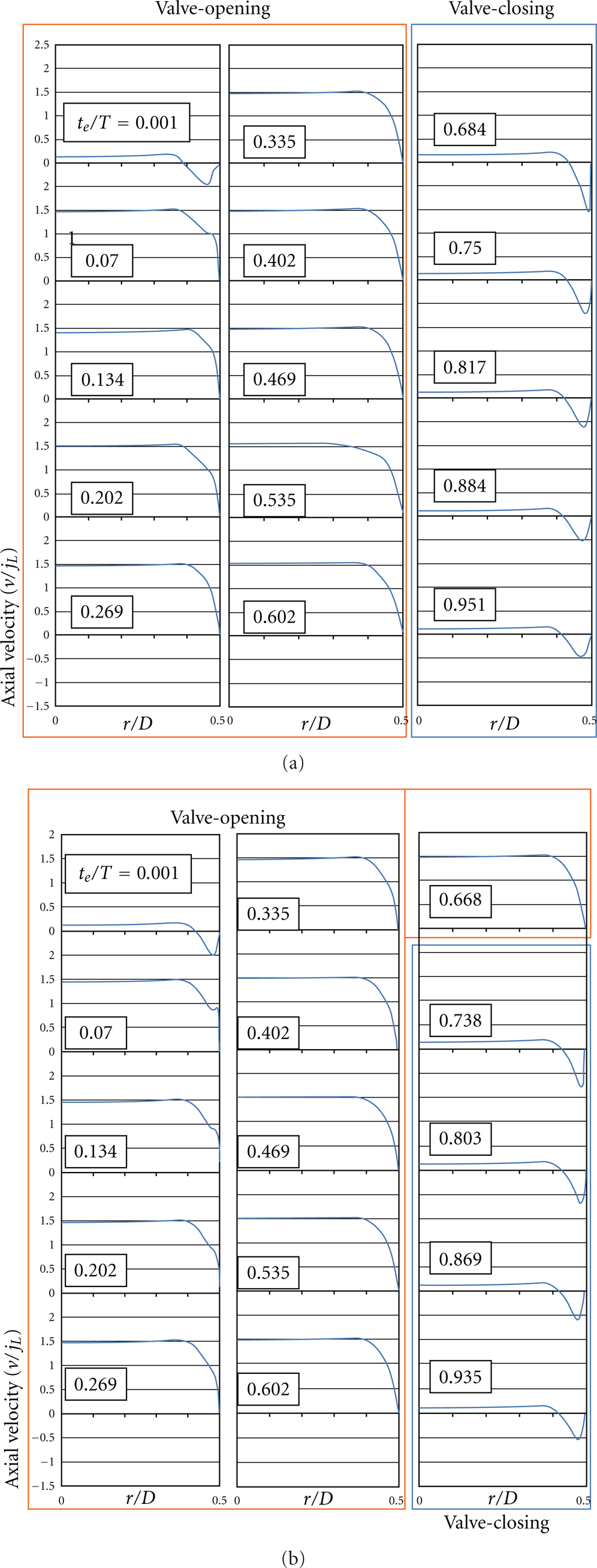
The simulations were conducted under the present experimental conditions. Figure 16 shows the time evolution of the dimensionless axial velocity distribution of water in the radial direction near the outlet of the pipe during one pulsation cycle in periodic motion. The flow conditions are (a) F = 3.33 Hz, V = 0.5, and j_L = 0.52 m/s and (b) F = 6.67 Hz, V = 0.363, and j_L = 0.43 m/s. In all cases, C_ratio = 0 and the pipe diameter is 18 mm. When the valve is activated and the inflow of liquid starts (t_e/T = 0.001), the axial velocity component is very small in the center region and negative velocity appears near the pipe wall. The velocity increases rapidly in the center region and soon reaches a constant value of v/j_L ∼ 1.5(t_e/T = 0.07–0.668). During the valve closing indicated by the blue line in the figure, the velocity becomes very small in the center region. Near the pipe wall, downward flow (reverse flow) arises. At any time, the calculated velocity profile is almost uniform in the center region.

Time evolution of axial velocity distribution in radial direction near outlet of pipe for (a) F = 3.33 Hz, V = 0.5, and j_L = 0.52 m/s and (b) F = 6.67 Hz, V = 0.363, and j_L = 0.43 m/s.

We carried out various numerical simulations by varying the pulsation patterns and found that the occurrence of reverse flows is a characteristic feature of pulsating pipe flows. An additional experiment was performed to confirm the presence of reverse flows. In the present study, the pulsating flow was introduced by using an electromagnetic valve, as previously explained. The pressure at the valve changes considerably at every valve activation, resulting in the formation of cavitation bubbles. Thus, a small number of air bubbles with a diameter of 0.2–0.5 mm were always present in the pipe flows. Since the motion of such small bubbles follows the local liquid velocity well, the bubble motion is observed instead of the local liquid velocity. Figure 17 shows the time variation of the axial position of a small bubble in the vicinity of the pipe wall. The experimental conditions are the same as those in Figure 16(b). It should be noted that the velocity of the bubbles is much higher than that of the particles and the displacement is much larger as well. Thus, the bubble could be tracked for at most one pulsation cycle in the videography. The bubble moves upward during the valve opening. It goes downward during the valve closing, suggesting that downward flow is present in the vicinity of a pipe wall.

Figure 17

Axial position of small bubble in vicinity of pipe wall for F = 6.67 Hz, V = 0.363, C_ratio = 0.0, and j_L = 0.43 m/s.

According to the experimental results in Figure 10, the particles near the pipe wall begin to move radially inward immediately after the valve-closing. Such particle motion can be explained by the occurrence of the reverse flow. The abrupt occurrence of the reverse flow gives rise to a large temporary drag force acting on the particles. The direction of the drag force is inward, opposite to that of the steady-flow case. As a consequence, in pulsatile flows the particles are pushed inward and frequently pass near the center axis.

In the previous section discussing the one-dimensional simulations for tracking particles (Figure 13), the predictions agree reasonably well with the experiments for C_ratio = 0.0 m/s, but an appreciable difference was seen for large C_ratio. This can be explained using the results of the numerical simulations. Figure 18 shows the mean velocity profiles of the liquid near the outlet of the pipe for F = 3.33 Hz, V = 0.5, and j_L = 0.52 m/s. The value of C_ratio was varied as a parameter. The predicted mean velocity profile was calculated as

\bar{v} (r) = \frac{1}{T} \int_{t_{i}}^{t_{i} + T} v (r, t) d t,

(23)

where t_i is 3.0 s, the time at which the calculated flow shows periodic motion. The mean velocity at the center axis decreases with decreasing C_ratio and the velocity profile becomes flat. For small C_ratio, the liquid velocity profile is almost uniform and the one-dimensional flow assumption is appropriate except near the pipe wall. In contrast, the assumptions are invalid for large C_ratio. Thus, the one-dimensional model failed to predict the particle motion.

Figure 18

Mean velocity profiles of liquid near outlet of pipe for F = 3.33 Hz, V = 0.5, and j_L = 0.52 m/s.

5.5. Critical Minimum Water Flux for Pulsating Pipe Flows

The critical water fluxes in pulsation flows are now discussed. Table 3 shows the critical water flux, j_L,min, for d = 5 mm, D = 22 mm, and V = 0.5. The frequency ranged from 3.33 Hz to 6.67 Hz and the water temperature was 20°C. The flux of the constant flow j_L,C associated with C_ratio was varied as a parameter. It was found that the critical water flux increases with increasing j_L,C. The mechanism can be explained as follows. The velocity change in the liquid during one pulsation cycle decreases with increasing j_L,C and the flows come close to the steady state for large j_L,C. For small j_L,C (or C_ratio), the particles can pass in the center region where the liquid velocity is large, as previously discussed. In contrast, for large j_L,C (or C_ratio) the particles move near the pipe wall where the local liquid velocity is small (see also Figure 12). As a result, the critical water fluxes for steady flows are larger than those for pulsating flows with small C_ratio. In addition, the effect of frequency on the critical flux is seen for small j_L,C.

Table 3:

Critical minimum water flux for alumina particle with diameter of 5 mm.

	j_LC = 0.10 m/s	j_LC = 0.30 m/s	j_LC = 0.50 m/s

F = 3.33 Hz	0.50 m/s	0.52 m/s	0.52 m/s
F = 4.16 Hz	0.47 m/s	0.52 mm	0.52 m/s
F = 6.67 Hz	0.42 m/s	0.47 mm	0.52 m/s

Figure 19 shows the critical minimum water fluxes j_L,min for (a) d = 3 mm and (b) d = 5 mm. The experimental conditions were C_ratio = 0, D = 18 mm, and a water temperature of 15°C. The critical fluxes decrease with increasing frequency. According to the experimental results in Figures 9(c) and 9(d), the chance of particles passing in the center region is higher for a larger frequency, because the reverse flow occurs more frequently. Since the liquid velocity is large in the center region and small in the vicinity of the pipe wall, the critical minimum water flux becomes small with increasing frequency of pulsation.

Critical minimum water fluxes under various pulsating flow conditions.

The critical fluxes also decrease with increases in the V values. This can be explained using the results of the numerical simulations. Figure 20 shows a comparison of the time variation of the axial velocity distribution in the radial direction near the outlet of the pipe. The flow conditions are (V, F, C_ratio,j_L) = (1.0, 3.33 Hz, 0, 0.52 m/s) and (0.15, 3.33 Hz, 0, 0.52 m/s). The reverse flow occurs for a longer period for a larger V value. The peak velocity of the reverse flow is also larger. Thus, the radially inward drag force acts on a particle near the pipe wall more appreciably for a larger V value, and the chance of particles being located in the center increases. The experimental data in Figures 9(a) and 9(b) are consistent with this explanation. Consequently, the critical minimum water flux becomes small with increasing V.

Figure 20

Effect of V value on calculated velocity profile for F = 3.33 Hz, C_ratio = 0.0, and j_L = 0.52 m/s.

6. Conclusions

The transport characteristics of single solid particles in pulsating pipe flows were investigated. The three-dimensional particle motion was observed using two digital video cameras. Further, two types of numerical simulations were carried out. The main results are summarized below.

The particle is lifted upward along the pipe wall in steady upward flows because of the vertical velocity profile of the liquid in the radial direction. In pulsating upward flows, the particle moves upward with an up-and-down motion. The particle was located near the pipe wall and then near the center axis, because of the occurrence of reverse flow near the pipe wall.

The numerical simulations revealed that the liquid velocity profile is almost flat near the center axis in the pulsating pipe flows at small C_ratio. In such a case, the one-dimensional simulations carried out for tracking the particle motion are valid. With increasing C_ratio and V values, the liquid mean velocity profile approaches the steady-state distribution.

The critical minimum flux for transporting single particles depends on the pulsating pattern. Under the present experimental conditions, the critical fluxes decrease with decreases in C_ratio, with increases in F, and with increases in V.

References

Fujimoto

Ogawa

Takuda

, and Hatta

, “Operation performance of a small air-lift pump for conveying solid particles,” Journal of Energy Resources Technology, vol. 125, no. 1, pp. 17–25, 2003.

Fujimoto

Murakami

Omura

, and Takuda

, “Effect of local pipe bends on pump performance of a small air-lift system in transporting solid particles,” International Journal of Heat and Fluid Flow, vol. 25, no. 6, pp. 996–1005, 2004.

Fujimoto

Nagatani

, and Takuda

, “Performance characteristics of a gas-liquid-solid airlift pump,” International Journal of Multiphase Flow, vol. 31, no. 10–11, pp. 1116–1133, 2005.

Hatta

Omodaka

Nakajima

Takatsu

Fujimoto

, and Takuda

, “Predictable model for characteristics of one-dimensional solid-gas-liquid three-phase mixtures flow along a vertical pipeline with an abrupt enlargement in diameter,” Journal of Fluids Engineering, vol. 121, no. 2, pp. 330–342, 1999.

Kato

Miyazawa

Timaya

, and Iwasaki

, “A study of an air-lift pump for solid particles,” Bulletin of the JSME, vol. 18, no. 117, pp. 286–294, 1975.

Weber

and Dedegil

M. Y.

, “Transport of solids according to the air-lift principle,” in Proceedings of the 4th International Conference on the Hydraulic Transport of Solids in Pipes, pp. H1-1-23–X93-94, Alberta, Canada, 1976.

Yoshinaga

and Sato

, “Performance of an air-lift pump for conveying coarse particles,” International Journal of Multiphase Flow, vol. 22, no. 2, pp. 223–238, 1996.

Kassab

S. Z.

Kandil

H. A.

Warda

H. A.

, and Ahmed

W. H.

, “Air-lift pumps characteristics under two-phase flow conditions,” International Journal of Heat and Fluid Flow, vol. 30, no. 1, pp. 88–98, 2009.

Ramaprian

B. R.

and Tu

S. W.

, “An experimental study of oscillatory pipe flow at transitional Reynolds numbers,” Journal of Fluid Mechanics, vol. 100, no. 3, pp. 513–544, 1980.

10.

S. W.

and Ramaprian

B. R.

, “Fully developed periodic turbulent pipe flow. Part 1. Main experimental results and comparison with predictions,” Journal of Fluid Mechanics, vol. 137, pp. 31–58, 1983.

11.

Ramaprian

B. R.

and Tu

S. W.

, “Fully developed periodic turbulent pipe flow. Part 2. The detailed structure of the flow,” Journal of Fluid Mechanics, vol. 137, pp. 59–81, 1983.

12.

Shemer

Wygnanski

, and Kit

, “Pulsating flow in a pipe,” Journal of Fluid Mechanics, vol. 153, pp. 313–337, 1985.

13.

Hwang

J. L.

and Brereton

G. J.

, “Turbulence in high-frequency periodic fully-developed pipe flow,” in Proceedings of the 8th International Symposium on Turbulent Shear Flows, pp. 11-3-1–11-3-6, Springer, Munich, Germany, September 1991.

14.

Brereton

G. J.

and Mankbadi

R. R.

, “Review of recent advances in the study of unsteady turbulent internal flows,” Applied Mechanics Reviews, vol. 48, no. 4, pp. 189–212, 1995.

15.

Eguchi

Watanabe

Takahara

, and Furukawa

, “Development of pulsatile flow experiment system and PIV measurement in an elastic tube,” Memoirs of the Faculty of Engineering, Kyushu University, vol. 63, no. 3, pp. 161–172, 2003.

16.

Ünsal

and Durst

, “Pulsating flows: experimental equipment and its application,” JSME International Journal, Series B, vol. 49, no. 4, pp. 980–987, 2007.

17.

and Jackson

J. D.

, “An experimental study of pulsating turbulent flow in a pipe,” European Journal of Mechanics, B/Fluids, vol. 28, no. 2, pp. 309–320, 2009.

18.

Ariyaratne

, and Vardy

A. E.

, “A computational study of wall friction and turbulence dynamics in accelerating pipe flows,” Computers & Fluids, vol. 37, no. 6, pp. 674–689, 2008.

19.

Blel

Le Gentil-Lelièvre

Bénézech

Legrand

, and Legentilhomme

, “Application of turbulent pulsating flows to the bacterial removal during a cleaning in place procedure. Part 1: experimental analysis of wall shear stress in a cylindrical pipe,” Journal of Food Engineering, vol. 90, no. 4, pp. 422–432, 2009.

20.

Akhremenko

A. I.

Belousov

V. L.

, and Marchenkov

V. P.

, “Theoretical studies of transport of solid particles in pulsating flows,” Journal of Engineering Physics and Thermophysics, vol. 68, no. 2, pp. 176–181, 1995.

21.

Suzuki

Hasegawa

, and Matsufuji

, “Motion of small particles due to a pulsatile flow in a chamber,” JSME International Journal, Series B, vol. 36, no. 1, pp. 57–65, 1993.

22.

Carvalho

J. A.

Jr. , “Behavior of solid particles in pulsating flows,” Journal of Sound and Vibration, vol. 185, no. 4, pp. 581–593, 1995.

23.

Saito

Kajishima

Kiyono

, and Usami

, “Particle velocity in the main stream direction of solid-liquid two-phase flows in a swaying pipe,” Transactions of the Japan Society of Mechanical Engineers. B, vol. 59, no. 563, pp. 29–34, 1993.

24.

Eesa

and Barigou

, “CFD investigation of the pipe transport of coarse solids in laminar power law fluids,” Chemical Engineering Science, vol. 64, no. 2, pp. 322–333, 2009.

25.

El Masry

O. A.

and El Shobaky

, “Pulsating slurry flow in pipelines,” Experiments in Fluids, vol. 7, no. 7, pp. 481–486, 1989.

26.

Clift

Grace

J. R.

, and Weber

M. E.

, Bubbles, Drops, and Particles, Academic Press, San Diego, Calif, USA, 1978.

27.

Takewaki

and Yabe

, “The cubic-interpolated pseudo particle (CIP) method: application to nonlinear and multidimensional hyperbolic equations,” Journal of Computational Physics, vol. 70, no. 2, pp. 355–372, 1987.

Transport Phenomena of Solid Particles in Pulsatile Pipe Flow

Abstract

1. Introduction

2. Literature Survey

3. Setup

3.1. Experimental Apparatus

3.2. Videography and Data Reduction for Particle Motion

4. Numerical Procedure

4.1. One-Dimensional Simulation of Particle Motion

4.2. Two-Dimensional Simulation for Analyzing Liquid Pipe Flows

5. Results and Discussion

5.1. Videographic Observation of Particle Motion in Steady Pipe Flows

5.2. Videographic Observation of Particle Motion in Pulsatile Pipe Flows

5.3. One-Dimensional Simulation for Tracking Particle Trajectory

5.4. Two-Dimensional Simulation for Pulsating Pipe Flows

5.5. Critical Minimum Water Flux for Pulsating Pipe Flows

6. Conclusions

References