Sage Journals: Discover world-class research

Abstract

This paper discusses a finite element analysis of the Bauschinger effect in the reverse cup drawing process, taken from the NUMISHEET′99 (Gelin and Picart, 1999) benchmark. In order to study the Bauschinger effect, several hardening models are considered such as isotropic, kinematic, and combined forms in the linear and nonlinear cases, including the well-known Yoshida and Chaboche's model. The obtained results have been compared with some experimental results reported in literature. The various factors, namely, normalized axial stress, von Mises stress, and the punch forces, for both first and second stages have been calculated for different materials and thicknesses. Results show that the combined model had acceptable agreement with the empirical data through both stages, while the bilinear models did not show this effectiveness. Generally, the nonlinear kinematic and combined models lead to more accurate results.

1. Introduction

During deformation of metals at room temperature, usually their resistance against deformation increases in a process known as work hardening. There are different theories for predicting this phenomenon in different materials, that is, isotropic hardening and kinematic hardening [1]. The isotropic hardening theory, as the simplest hardening theory, assumes that the size of yield surface during plastic deformation increases but it does not move in the space of stresses. The amount of increase in size depends on only one parameter which is controlled by plastic deformation [2] (Figure 1).

Figure 1:

The sketch of isotropic hardening in stress space.

On the other hand, the kinematic hardening rule assumes that during plastic deformation, the yield surface moves in the stress space as a rigid body but without any change in orientation. Therefore the size, shape, and orientation of the initial yield surface are fixed. This hardening rule provides a simple method to consider the Bauschinger effect and the yield surface transfers in the principal stresses space in the direction of plastic strain [3].

1.1. Reverse Plasticity Models

In the kinematic hardening rule, the initial yield surface is represented by equation f(σ_{i
j}) = k² where k is a constant. If the resultant displacement of yield surface at any stage is denoted by a symmetrical tensor α_{i
j}, the current yield surface is given by

f (σ_{i j} - α_{i j}) = k^{2} .

(1)

The incremental movement of the yield surface in the direction of plastic increment is a vector in the space. Then,

d α_{i j} = c d {ε_{i j}}^{p},

(2)

where c defines material behavior. If deformation is too small, the effect of element rotation on dα_{i
j} will be ignored. This hardening rule is shown in Figure 2 where O is the center of stress space and c is the current center of yield surface. The incremental translation of the yield surface during a stress increment pp^′ is represented by cc^′, which is parallel and equal to PQ. When c is constant, the total translation of the yield surface is a measurement of the total plastic strain. In addition, if the initial surface is that of von Mises, the yield criterion becomes

Figure 2:

The sketch of prager hardening in stress space.

(s_{i j} - c {ε^{p}}_{i j}) (s_{i j} - c {ε_{i j}}^{p}) = 2 k^{2},

(3)

where k is the initial yield stress in pure shear. A constant value of c represents a linear strain-hardening with a plastic modulus of $H = 3 c / 2$ .

In many cases the yield surface undergoes translation but in a direction different from the outward normal which is know as zeigler hardening [4, 5]:

d α {}_{i j} = (σ_{i j} - α_{i j}) d μ,

(4)

where dμ is a positive scalar. This equation states that the yield surface translates in the direction of a line connecting the center of the yield surface to the current stress point p (Figure 3). Moreover, the incremental translation of the yield surface is represented by the vector cc^′, equal to the vector PQ, where Q lies on CP extended. Thus,

Figure 3:

The sketch of ziegler hardening in stress space.

(d σ_{i j} - d α_{i j}) d {ε_{i j}}^{p} = 0 .

(5)

By substituting(5) into (4) we get,

d μ = \frac{d σ_{i j} d {ε_{i j}}^{p}}{(σ_{k l} - α_{k l}) d {ε_{k l}}^{p}} .

(6)

In recent years, various hardening models have been presented by some researchers. Armstrong and Fredrick proposed a nonlinear kinematic hardening [4]. In their model, the effect of strain path, the anisotropy property in compression-tension curve, and the movement of yield surface during loading and unloading in stress space were investigated.

Hu et al. (1992) [6] and Hu (1994) [7] have proposed a uniaxial constitutive model of large-strain plasticity that may describe the work hardening stagnation as well as the cyclic strain-range dependency of stress amplitude. Later on, Teodosiu et al. (1997) [8] generalized that model for multiaxial plasticity. Although their models can simulate the transient Bauschinger effect and the behavior of work hardening stagnation, they did not pay much attention to the accurate description of the stress-strain in the small-scale re-yielding region, which is essential for the springback prediction [9]. Yoshida proposed a constitutive model of plasticity within the framework of well-known two surface modeling, wherein the yield surface moves kinematically within a bounding surface [10, 11]; see Figure 4. As well as for the global cyclic hardening behavior, it is very important to simulate precisely the transient Bauschinger deformation, especially for the purpose of accurate prediction of springback in sheet metal forming. The stress-strain responses during the transient period calculated by Yoshida-Uemori and the IH + NLK (isotropic hardening + nonlinear kinematic) models are different as can be seen in Figure 5 [12].

Figure 4:

Schematic illustration of two-surface model.

Figure 5:

Stress-strain responses during the transient Bauschinger deformation calculated by Yoshida-Uemori and the IH + NLK model, together with experimental results.

Chun modified the changes of stress level by isotropic hardening [13, 14]. His model can predict the behavior of material better compared to the experimental results. Recently, other researchers have studied the reverse plasticity by different hardening models [15–19].

Reverse cup drawing is a remarkable process that may be investigated by using different theories. For this purpose, the recognition of these models may have a main role to help one to achieve an accurate simulation. In order to study the deep drawing process in thin sheets, using of a proper hardening model, as mentioned in the previous part, is essential. The purpose of this paper is to investigate the accuracy of various plasticity constitutive models in reverse forming of thin sheets. Thus, different sheets with a variety of thicknesses have been used in our simulations. To treat the nonlinear elastic-plastic problem the commercial finite element code, Ansys 6.1 (ANSYS 6.1 User Manual), is used.

2. Method of Simulation

The reverse cup drawing test (Figure 6) is composed of two stages, that is, forward drawing and reverse drawing, with fixed gaps between the die and blank holder. Two die gaps have to be chosen properly enabling the drawing process to be performed without any wrinkles or failure. In the current simulation, a fixed gap condition is applied instead of forces. For instance, a constant blank holder force has to be applied to keep the gap constant: approximately 1.22 and 1.32 mm for the first and second stages, respectively. The friction coefficient is assumed to be uniform and constant for all contacting surfaces and equal to 0.168 [13, 14]. The simulation may be performed in 2D because of its axial symmetry and a visco solid 106 element can be used for the sheet. Contact 172 element has been used for deformable surfaces and Target 169 element for rigid surfaces. Figure 7 illustrates the geometry, node location, and coordinate system for visco solid and contact elements. Figure 8 shows that the elements of different parts have acceptable conformity with each other to obtain best accuracy during reverse cup drawing test.

Figure 6:

Geometry and dimensions for reverse cup drawing test: (a) at the start of the first stage, and (b) at the start of the second stage.

Figure 7:

Different appliedelements: (a) visco solid element, (b) contact 171 element, and (c) target 169 element.

Figure 8:

Schematic of model optimum meshing: (a) first punch and sheet, and (b) second punch and matrix.

The punch force is applied using the displacement of the punches. At the end of the first stage, the first punch becomes stationary and plays the role of a holder, while the second punch moves upwards. The mesh grid is of “free” type and the grid lines have been placed so that the elements are as close to squares as possible. The mesh grid is of the highest importance because in the reverse process, the change in shape of the elements causes the process not to converge easily. To examine the legitimacy of the mesh grid, a sample point is considered at a distance of 64.5 mm from the axis of symmetry. Figure 9 shows sample point on model with the symmetry boundary conditions along x-and y-axis.

Figure 9:

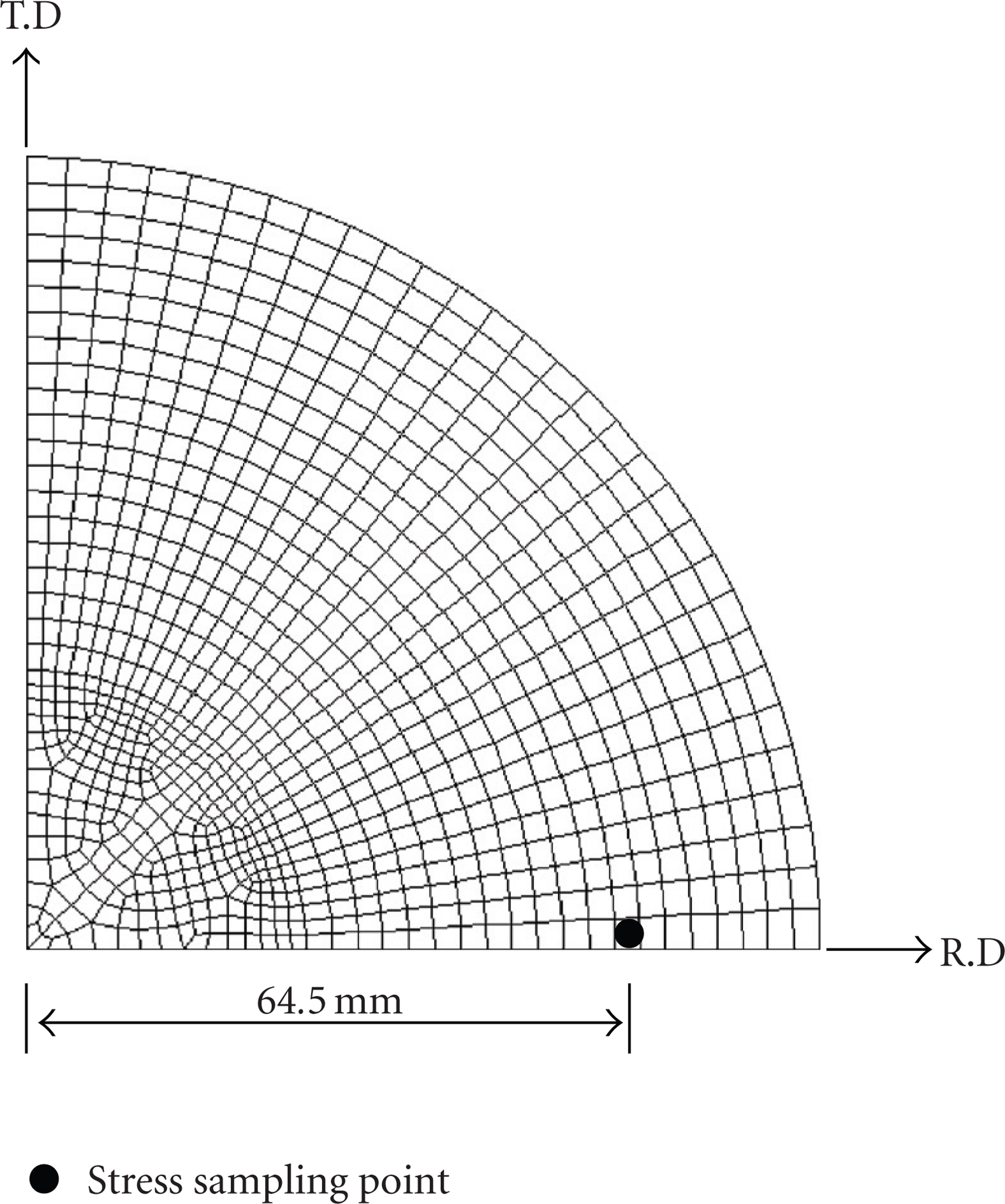
Finite element mesh and stress sampling point for the reverse cup drawing process simulation.

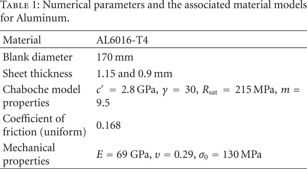
The entire parameters of the process, including stresses, have been investigated at this point in detail. In this simulation, various hardening models are used for large deflection problems so that the differences between these models can be observed. The utilized material is AL6016-T4 and its basic properties are shown in Table 1. The Ansys code is used for simulations with different hardening models such as Chaboche-nonlinear isotropic (Nonlinear Isotropic) combined model and isotropic hardening in both linear and nonlinear types (LIso, NIso).

Table 1:

Numerical parameters and the associated material models for Aluminum.

Material	AL6016-T4

Blank diameter	170 mm
Sheet thickness	1.15 and 0.9 mm
Chaboche model properties	c^′ = 2.8 GPa, γ=30, R_sat = 215 MPa, m = 9.5
Coefficient of friction (uniform)	0.168
Mechanical properties	E = 69 GPa, υ=0.29, σ₀ = 130 MPa

3. Results and Discussions

Figure 10 shows the deformed shapes of an experimental specimen at three different stages, and the comparison with the simulated results is shown in Figure 11.

Figure 10:

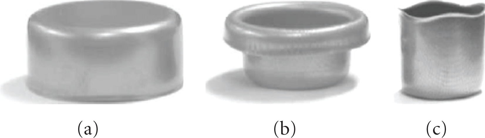
Predicted deformed shapes in the reverse cup drawing process for AL6016-T4: (a) after the first stage, (b) with 50 mm punch travel in the second stage, and (c) after the second stage.

Figure 11:

Simulated deformed shapes in the reverse cup drawing process for AL6016-T4: (a) after the first stage, (b) with 55 mm punch travel in the second stage, and (c) after the second stage

The obtained axial stresses from the Chaboche-nonlinear isotropic combined models and the nonlinear isotropic are different at both stages as shown in Figure 12. In order to demonstrate the normalized axial stress, the axial stress is divided by yield stress; the stresses in the rolling direction are taken at the sample point for seven steps of deformation stages. The obtained results show that the element is initially in tension (at the deformation steps 0–0.7) and is subsequently compressed as it passes over the die shoulder (steps 0.7–1.2). However, the axial stresses computed by the two hardening models show some differences from this stage (step 1.2). Slight retension and compression is repeated due to straightening at the side wall (steps 1.2–3). When this point passes over the die shoulder again, during the second stage, the load reversal is more pronounced (steps 3–7). The overall trend of the Chaboche-nonlinear isotropic combined model is to predict lower of axial stress due to the permanent softening characteristic at the reversal straining.

Figure 12:

Normalized axial stress at the selected point in the reverse cup drawing process with AL6016-T4.

Figure 13 shows a favorable comparison between an experimental punch force–displacement results and the prediction obtained from the Chaboche-nonlinear isotropic combined model [13, 14]. This model predicted slightly lower maximum of punch forces, compared to the experimental data in the both first and second stages; see Figure 13 and Table 2. The differences in the compared results may be due to the simulation of boundary conditions. For instance, the simulation is performed under a fixed gap condition, and the blank-holder force is applied to keep the gap approximately fixed in the test. Other obtained errors may be attributed to the yield criterion, friction effects, and contact treatment. Concerning the effect of material type modeling, it is important that different material models produce different resulting stress distributions with similar strain path, which leads to different force–displacement curves. Generally, the Chaboche-nonlinear isotropic combined model predicted the maximum punch forces more accurately for the reverse cup drawing process.

Table 2:

Maximum punch forces in reverse cup drawing process.

Different states	Maximum punch (kN) forces
Different states	First Stage	Second stage

Experimental	62	55
Chaboche and NLIso model	61	52
NLIso model	68	59
LIso model	70	62

Figure 13:

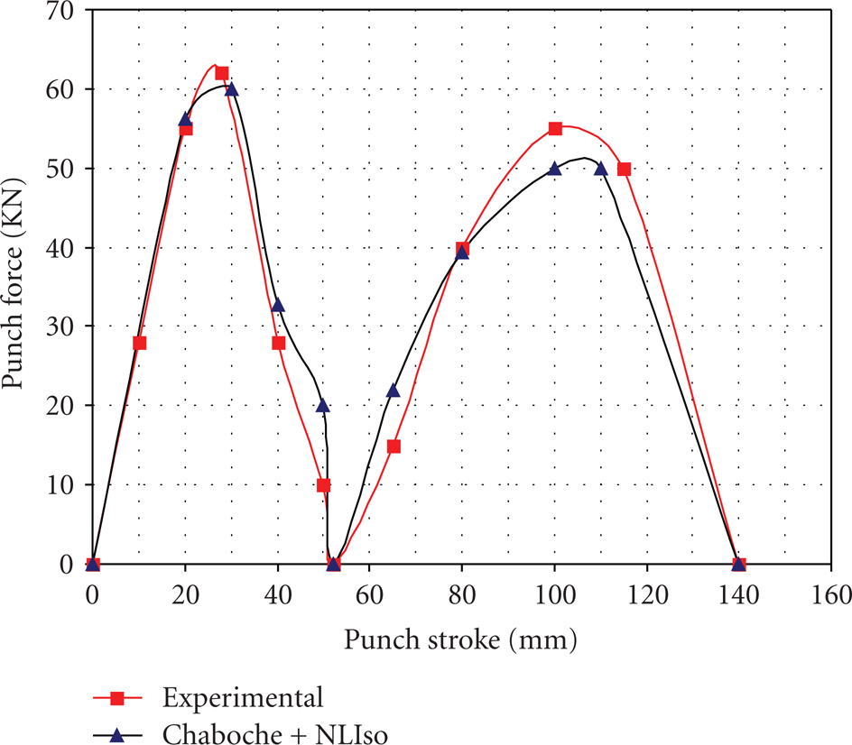
Comparison of force-displacement curves during the first and second stage in the reverse cup drawing process with AL6016-T4.

Figure 14 compares the computed thickness distributions with experimental results along the 45 degree line from the rolling direction at first stage (Figure 14(a)) and second stage (Figure 14(b)). Two hardening models predicted very similar thickness distribution because the stretching is a dominant made of deformation.

Figure 14:

Thickness distribution along 45 degree from the rolling direction: (a) first stage, (b) second stage.

Figure 15:

Von Mises stress at sample point for various hardening models.

Figure 15 shows the normalized von Mises stress, (divided by yield stress), for three hardening models during loading. The linear isotropic hardening cannot predict the behavior of materials precisely and effective stress in material exceeds the yield stress and material will fail during loading according to this model. The other two models almost show similar behavior. An investigation into the effect of sheet thickness has also been carried out and the results are demonstrated in Figure 16. Two different thicknesses (0.9 and 1.15 mm) with Chaboche-nonlinear isotropic combined model are used, and the difference between the required forces during the forming process is illustrated in this figure. The predicted punch forces by two models shows practically low difference.

Figure 16:

Comparison of force–displacement curves during the first and second stages in the reverse cup drawing process for two thicknesses (AL-Chaboche-Nliso model).

4. Conclusions

A forming process consisting of reverse bending was selected and examined through a series of studies and simulations. Three hardening models, that is, bilinear isotropic, nonlinear isotropic, and Chaboche-nonlinear isotropic combined were numerically evaluated through the reverse cup drawing test. The effectiveness of Chaboche-nonlinear isotropic model in predicting the behavior of materials with Bauschinger effect was considerable. In this simulation, the predicted thickness distribution by two models shows practically no difference. However the resulting stresses and punch forces are quite different. The combined model had acceptable agreement with measured date through two stages, while the bilinear models did not show this effectiveness. Generally, the nonlinear isotropic and combined models produced more accurate results.

References

Chakrabarty

, Theory of Plasticity, McGraw-Hill, New York, NY, USA, 1989.

Chen

W. F.

, Constitutive Equations for Engineering Materials, McGraw-Hill, New York, NY, USA, 1994.

Johnson

and Mellor

P. B.

, Engineering Plasticity, John Wiley & Sons, New York, NY, USA, 1983.

Armstrong

P. J.

and Frederick

C. O.

, “A mathematical representation of the multiaxial Bauschinger effect,” GEGB Report RD/B/N731, Berkeley Nuclear Laboratories.

Chaboche

J. L.

, On the Constitutive Equations of Materials under Monotonic or Cyclic Loading, Engineer, Head Research Section, ONERA Structures Department, 1983.

Rauch

E. F.

, and Teodosiu

, “Work-hardening behavior of mild steel under stress reversal at finite strains,” International Journal of Plasticity, vol. 8, pp. 839–856, 1992.

, “Work-hardening behavior of mild steel under cyclic deformation at finite strains,” Acta Metallurgica et Materialia, vol. 42, no. 10, pp. 3481–3491, 1994.

Teodosiu

Duval

J.-L.

, and Haddadi

, “Modelling the microstructural evolution during large plastic deformations,” in Proceedings of the IUTAM Symposium on Micro- and Macrostructural Aspects of Thermoplasticity, Bruhns

O. T.

and Stein

, Eds., pp. 479–488, Kluwer Academic Publishers, 1997.

Yoshida

, “A constitutive model of cyclic plasticity,” International Journal of Plasticity, vol. 16, no. 3–4, pp. 359–380, 2000.

10.

Yoshida

and Uemori

, “A model of large-strain cyclic plasticity describing the Bauschinger effect and workhardening stagnation,” International Journal of Plasticity, vol. 18, no. 5–6, pp. 661–686, 2002.

11.

Yoshida

Uemori

, and Fujiwara

, “Elastic-plastic behavior of steel sheets under in-plane cyclic tension-compression at large strain,” International Journal of Plasticity, vol. 18, no. 5–6, pp. 633–659, 2002.

12.

Yoshida

and Uemori

, “A model of large-strain cyclic plasticity and its application to springback simulation,” Key Engineering Materials, vol. 233–236, no. 1, pp. 47–58, 2002.

13.

Chun

B. K.

Jinn

J. T.

, and Lee

J. K.

, “Modeling the Bauschinger effect for sheet metals—part I: theory,” International Journal of Plasticity, vol. 18, no. 5–6, pp. 571–595, 2002.

14.

Chun

B. K.

Kim

H. Y.

, and Lee

J. K.

, “Modeling the Bauschinger effect for sheet metals—part II: applications,” International Journal of Plasticity, vol. 18, no. 5–6, pp. 597–616, 2002.

15.

Gau

J.-T.

and Kinzel

G. L.

, “An experimental investigation of the influence of the Bauschinger effect on springback predictions,” Journal of Materials Processing Technology, vol. 108, no. 3, pp. 369–375, 2001.

16.

Gau

J.-T.

and Kinzel

G. L.

, “A new model for springback prediction in which the Bauschinger effect is considered,” International Journal of Mechanical Sciences, vol. 43, no. 8, pp. 1813–1832, 2001.

17.

Tóth

L. S.

Molinari

, and Zouhal

, “Cyclic plasticity phenomena as predicted by polycrystal plasticity,” Mechanics of Materials, vol. 32, no. 2, pp. 99–113, 2000.

18.

Mahbadi

and Eslami

M. R.

, “Cyclic loading of beams based on the Prager and Frederick-Armstrong kinematic hardening models,” International Journal of Mechanical Sciences, vol. 44, no. 5, pp. 859–879, 2002.

19.

Yip

T.-H.

and Wang

, “Cyclic plasticity of precipitation-hardenable stainless steel,” Key Engineering Materials, vol. 233–236, pp. 275–280, 2003.

An Investigation into the Different Hardening Models in Reverse Forming of Thin Sheets

Abstract

1. Introduction

1.1. Reverse Plasticity Models

2. Method of Simulation

3. Results and Discussions

4. Conclusions

References