Sage Journals: Discover world-class research

Abstract

The elastic compensation method proposed by Mackenzie and Boyle is used to estimate the upper and lower bound limit (collapse) loads for one-piece aluminium aerosol cans, which are thin-walled pressure vessels subjected to internal pressure loading. Elastic-plastic finite element predictions for yield and collapse pressures are found using axisymmetric models. However, it is shown that predictions for the elastic-plastic buckling of the vessel base require the use of a full three-dimensional model with a small unsymmetrical imperfection introduced. The finite element predictions for the internal pressure to cause complete failure via collapse fall within the upper and lower bounds. Hence the method, which involves only elastic analyses, can be used in place of complex elastic-plastic finite element analyses when upper and lower bound estimates are adequate for design purposes. Similarly, the lower bound value underpredicts the pressure at which first yield occurs.

1. Introduction

The design of pressure vessels andrelated components is usually based on a combination of finite element analysis and rules contained within the appropriate codes of practice such as BS5500 [1] and ASME VIII [2] where yielding is generally considered to be the upper bound. Post-yield design is becoming more extensive, with techniques such as elastic-plastic finite element analysis being used in order to study shakedown and ratchetting regimes as well as collapse conditions. To avoid the added complexities of nonlinear analysis, a limit load approach has been suggested [3–6]. The lower limit is based on the lower-bound limit load theorem:

“If for a given loadP_L, a statically admissible stress field exists in which the stress nowhere exceeds the yield stress of the material, then P_L is a lower bound limit load.”

Correspondingly, the upper limit is based on the upper-bound limit-load theorem:

“If, for a given load set, the rate of dissipation of internal energy in a body is equal to the rate at which external forces do work in any postulated mechanism of deformation, the applied load set will be equal to or greater than the plastic collapse load.”

Direct calculation of limit loads using upper and lower bound theories is very difficult because it requires a statically admissible stress field and a kinematically admissible strain field. In order to determine the equilibrium equations between the external forces and internal stresses and the stress-strain relationships, a complicated collapse solution is required. To avoid this, several alternative approaches have been investigated; see review in [7]. The reduced modulus method (see, e.g., [8]) has been modified [9] such that

the elastic-plastic solution is replaced by a series of elastic solutions,

after each elastic computation, the modulus of elasticity is reduced until the conditions of admissible stress and strain fields, as lower and upper bound criteria, respectively, are satisfied.

This method has been further developed by Mackenzie and Boyle [10] and Mackenzie et al. [11], who have presented an elastic compensation method, where a series of elastic finite element analyses are used to predict a converged solution, which meets either the lower or upper bound criteria. Applications such as beams in bending and/or tension, nozzles in spheres, and torispherical heads are considered. Gowhari-Anaraki and Adibi-Asl have used the method to estimate upper and lower limit and shakedown loads for beam members and a thick sphere in [12].

Hardy et al. [13] have used the method to estimate upper and lower bounds for hollow tubes with axisymmetric internal projections under axial loading. They found that this method could be used successfully to determine upper andlower bounds for both limit and shakedown loading, when being compared with elastic-plastic finite element predictions. Pham [14] has re-examined the classical shakedown theorem due to Koiter [5] to include both shakedown and nonshakedown conditions. The use of more sophisticated material behavior models in shakedown analyses has also been investigated by Weichert and Hachemi [15].

Aerosol cans, which are thin-walled pressure vessels with a complex shape, are generally made of tin-plated steel or aluminium. In the former case, the cans are normally constructed from three components; the base, the cylinder, and the top, which are joined. Alternatively, aluminium cans are produced in one piece from a cylindrical slug, using the “back extrusion” process. Most cans have bases that curve inwards and this shape strengthens the structure of the can. The inverted base design is an inherent safety feature as it provides a natural pressure release mechanism in the event of a pressure overload, with “dome reversal” (which is a form of elastic-plastic buckling) of the base occurring. This sudden change in geometry (a) results in an immediate fall in pressure and (b) provides a visual indication, since the can is no longer stable. In order for this pressure release mechanism to be effective, the design must be such that “dome reversal” occurs at a pressure lower than the burst pressure.

In this paper, the elastic compensation method is used to estimate the upper and lower bound limit loads for aluminium aerosol cans subjected to internal pressure loading and the results are compared with elastic and elastic-plastic finite element predictions of yield and collapse pressures. This relatively straight-forward geometry has been used to further investigate the validity of the elastic compensation method. Seshadri and Kizhatil [16] have suggested that if the procedure cannot be verified for simple components, it is unsafe to use it for more complex design.

Initially, the wall of the can is assumed to be of constant thickness and results for six thickness values are presented using axisymmetric finite element models. A realistic thickness profile is also used in a seventh three-dimensional model. The results demonstrate the inability of the axisymmetric models to predict elastic-plastic buckling and the seventh three-dimensional model, with initial imperfection, is used in order to replicate this buckling mechanism.

2. Elastic Compensation Method

The aim of the method, as described in [10, 11], is to systematically redistribute the predicted stress field, while still remaining statically admissible, by carrying out an iterative elastic analysis and modifying the local elastic modulus at each stage. In the resulting linear elastic solution, the displacement and strain fields remain compatible and describe a geometrically possible deformation mode. Full details of the procedure are provided in [10, 11, 13] and a brief review of the method is given here.

An initial elastic finite element analysis is performed with an arbitrary load set (e.g., P_d), using the true modulus of elasticity for the material, E₀. This is taken to be the zeroth iteration in a series of linear elastic analyses. In each of the subsequent analyses, the elasticmodulus of each element is modified according to the equation

E_{i} = \frac{E_{i - 1} σ_{L}}{σ_{char}},

(1)

where subscript “i” is the current iteration number, σ_L is a limiting value of stress, and σ_char is some characteristic stress within the element. It is suggested that this limiting stress is related to the material yield stress, σ_y, by

σ_{L} = α σ_{y},

(2)

where αis an arbitrary constant between 0 and 1 (2/3 being found to provide suitable convergence). It is also suggested that the characteristic stress is the maximum (unaveraged) nodal equivalent stress associated with the element calculated in the previous iteration, defined as σ_i−1. Nodal values are selected, in preference to integration point values, because they are the direct output from the elastic analysis and can be easily extracted by the FORTRAN interface program that has been written, as discussed later. Hence the iteration on element modulus of elasticity becomes

E_{i} = \frac{2 E_{i - 1} σ_{y}}{3 σ_{i - 1}} .

(3)

The iterative procedure redistributes the stresses in the component and, over a number of iterations, the net effect is to decrease the maximum stress in the model to reach a converged constant value, σ_d.

2.1. Application to Lower Bound Limit Load

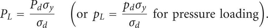
The lower bound limit load is calculated by applying the lower bound limit load theorem. The converged elastic compensation solution satisfies the first requirement of the lower bound theorem in that it is statically admissible. Because the solution is linear elastic, there is a linear relationship between stress and applied load. A lower bound load, P_L, can therefore be established as the load required to give a maximum (nodal equivalent) stress in the component/structure that is equal to the uniaxial yield strength of the material, σ_y. In a previous work (see [10]), it is argued that this lower bound load can be found from the proportionality relationship for the converged elastic solution (although other methods are possible), and hence for the worst point in the model and using this proportionality relationship:

\begin{array}{l} σ_{d} & = β P_{d}, \\ σ_{y} & = β P_{L} (where β is the constant of proportionality), \end{array}

(4)

hence

P_{L} = \frac{P_{d} σ_{y}}{σ_{d}} (or p_{L} = \frac{p_{d} σ_{y}}{σ_{d}} for pressure loading) .

(5)

The applied load set, P_d, is not restricted to single loads and may represent multiple forces, moments, pressure, and so forth, in the form of proportional loading.

2.2. Application to Upper Bound Limit Load

The upper bound limit load theorem for a complete plastic collapse solution can be expressed as (see [17])

\sum P \overset{\cdot}{u} = \int_{V} \overset{\cdot}{D} dV,

(6)

where $\overset{\cdot}{D}$ is the rate of dissipation of energy per unit volume, P is the set of equilibrium external loads, and $\overset{\cdot}{u}$ is the compatible set of displacement rates, which requires details of that complete plastic collapse solution.

Alternatively, an upper bound solution can be found when an incomplete or partial plastic collapse solution is available [11] and (6) can be rewritten in the form

\sum P \dot{u^{*}} \leq \int_{V} \overset{\cdot}{D^{*}} dV,

(7)

where the asterisk denotes an incomplete solution (i.e., a geometrically possible mode of deformation in which the stress field is not necessarily defined).

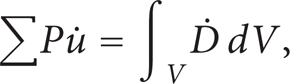
For this incomplete solution, compatible sets of displacements and strain increments are required and an iterative elastic finite element analysis, employing the elastic compensation method, will provide such information. However, the finite element predictions required to obtain the left-hand side of (7) are not always readily available. However, since the solutions are elastic, the elastic strain energy increment can be substituted, that is,

\int_{V} σ^{*} \dot{ε^{*}} dV \leq \int_{V} {\overset{\cdot}{D}}^{*} dV,

(8)

where σ* and $\overset{\cdot}{ε^{*}}$ are the elastically calculated stress and strain increment, respectively. Also, the increment of energy dissipation per unit volume for an elastic-perfectly plastic material, using the von-Mises yield criterion, can be expressed as [11]

\overset{\cdot}{D} = σ_{y} \sqrt{\frac{2}{3} ({\dot{ε}}_{1}^{2} + {\dot{ε}}_{2}^{2} + {\dot{ε}}_{3}^{2})},

(9)

where ${\dot{ε}}_{i}^{2} (i = 1, 2, 3)$ are the three principal strain rates.

Equation (8) can be rewritten in simple form as U≤D and, as shown in Figure 1, the dissipation energy, D, is linearly related to the applied load whereas the strain energy, U, varies with the square of the load. Furthermore, the intersection of the two lines represents the upper bound on the limit load.

Figure 1:

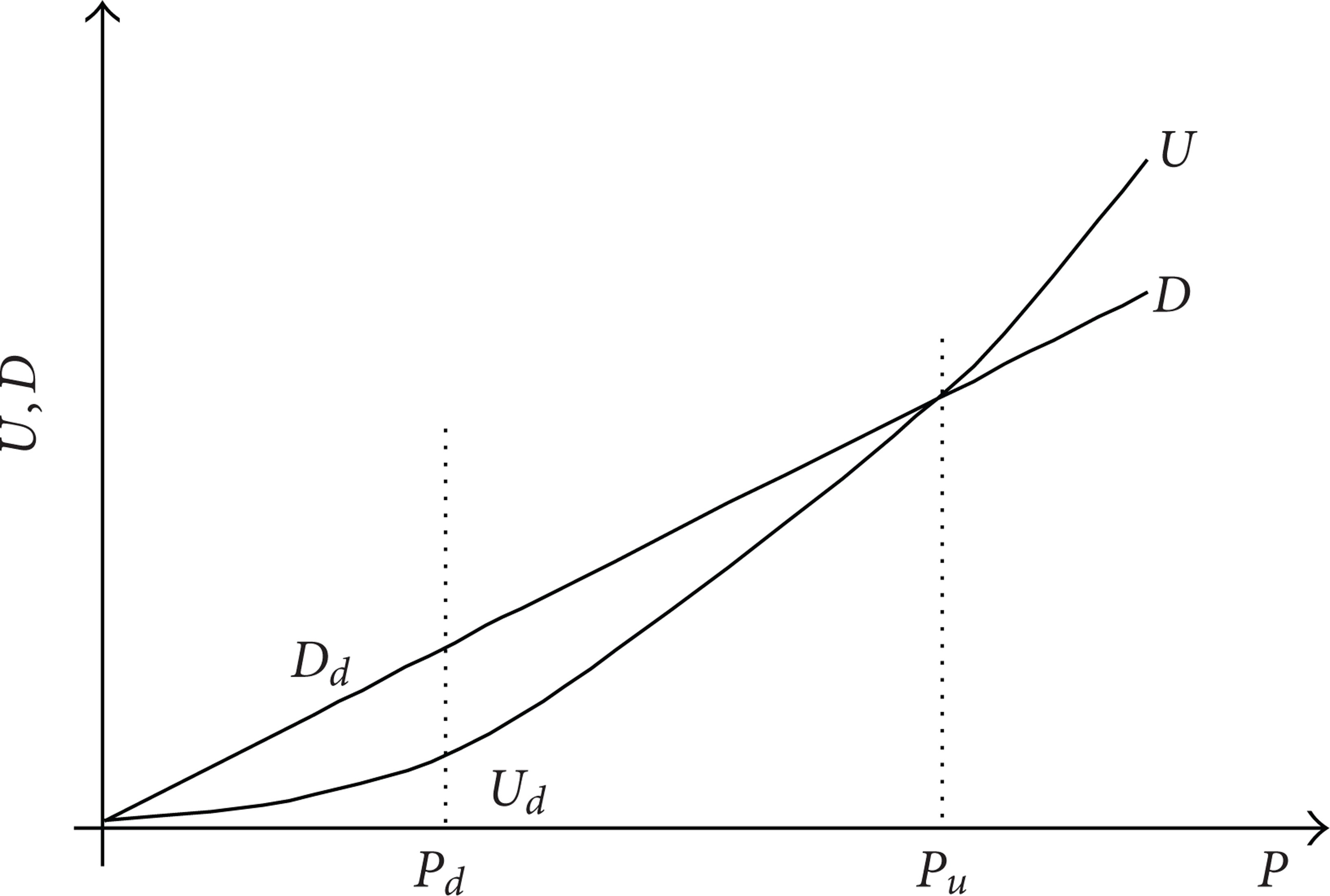
Variation in strain energy and dissipation energy with applied load, used in the calculation of the upper bound limit load.

The upper bound limit load is therefore obtained using predictions from the converged elastic compensation finite element solution with the arbitrary load set, P_d, that is,

\begin{array}{l} since U α P^{2}, D α P, \\ then U_{d} α P_{d}^{2}, D_{d} α P_{d} \end{array}

(10)

and because the solutions are elastic:

U = \frac{U_{d}}{P_{d}^{2}} P^{2}, D = \frac{D_{d}}{P_{d}} P for any load set, P .

(11)

Equating U and D at the upper bound limit load, P_u, gives

P_{U} = \frac{D_{d}}{U_{d}} P_{d},

(12)

where D_d and U_d are found from the converged elastic compensation finite element solution.

2.3. Method of Approach Using Finite Element Analysis

The procedure used in this approach is as follows [13].

Zeroth iteration. The initial elastic analysis is carried out with an arbitrary pressure, P_d, using E₀ throughout.

Store the elastic stress field, σ_e.

Identify the maximum stress in each element and use them to update elemental E values, using (3).

Identify the maximum stress in the model, σ_d.

Recreate the finite element program input data file, using the new E values.

ith iteration

(i)–(iv)

As above.

(v)

Compare σ_d with the value from the previous iteration (i.e., for convergence).

Converged solution. This occurs when σ_d becomes constant.

Calculate P_L using (5).

Obtain U_d and D_dfrom the finite element program output (see notes below).

Calculate P_U using (12).

2.4. Notes

(1) Strain energy values are obtained directly from the finite element program output file. The dissipation energy for each element is obtained from the three principal strain rates, the yield stress, and the element volume, using a version of (9) based on absolute values, not rates. A simple FORTRAN program was written to perform this calculation.

(2) The procedure in (i) to (iv) above is time consuming and prone to error, when performed manually. A FORTRAN program was written to perform these tasks automatically.

3. Finite Element Analysis (Constant Thickness Model)

A typicalbasic finite element model, made up of six “substructures”, for a can section that has a constant thickness of 1 mm is shown in Figure 2. Since the methodology involves an iterative finite element procedure, it was necessary to choose a mesh that meets both the condition of convergence and that of economy of the solution. A preliminary investigation, starting with a coarse mesh of 34 eight-noded axisymmetric elements (2 through-thickness), was undertaken in order to establish a suitable mesh for which mesh convergence had been reached. For the elastic compensation method analysis, 296 eight-noded, axisymmetric elements were generated manually from the basic mesh in Figure 2. On the basis of preliminary predictions, the cylindrical section was made long enough to ensure that a uniform stress was reached away from the discontinuities. The model is subjected to uniform internal pressure loading.

Figure 2:

Basic axisymmetric finite element model for can with constant thickness.

Finite element predictions have been obtained using the elastic (for compensation method) and large displacement elastic-plastic (for yield, elastic-plastic buckling and collapse) facilities of the ELFEN suite of programs [18]. Aluminium material property values for the true modulus of elasticity, E₀, yield stress, σ_y, and Poisson's ratio, ν, of 68.3 GPa, 100 MPa, and 0.3, respectively, were assumed. For the elastic-plastic analysis, an elastic-perfectly-plastic material model was assumed (for consistency with the plastic limit load theorem). In the elastic compensation analysis, an arbitrary pressure of 0.1 MPa has been used.

3.1. Elastic Analysis

Figure 3 shows the von-Mises equivalent stress contour plot for theinitial elastic solution (i.e., zeroth iteration in the elastic compensation method). Regions of above-average stress occur in the transition region between cylinder and base and at the base centre. By scaling up the results shown in Figure 3, where the maximum predicted stress is 13.25 MPa, an internal pressure at which first yield occurs was found to be 0.75 MPa.

Figure 3:

Equivalent stress contour plot for the zeroth iteration of the elastic compensation method with t=1 mm.

The iterative procedure described above has then been employed (with the aid of a FORTRAN program) and the modulus of elasticity in each element modified according to (3). The maximum equivalent stress at the end of each subsequent iteration is shown in Figure 4, from which it is clear that a converged solution occurs after 4 iterations with σ_d = 10.72 MPa. The elastic compensation method may, depending on the characteristic stress selected, cause the maximum stress to increase or decrease, but by careful selection, it is generally found that over a number of iterations there will be a net decrease in maximum stress with respect to the initial elastic solution.

Figure 4:

Maximum equivalent stress at the end of each iteration for t=1 mm.

The steady-state (converged) equivalent stress contour plot is shown in Figure 5. A redistribution of stress has occurred with an initial stress range of 0.22–13.25 MPa (seeFigure 3) reducing to 0.02–10.72 MPa. It is also apparent that the stress discontinuities at element boundaries have become more pronounced since the values of elastic modulus can now significantly vary from element to element. From (5), it follows that the predicted value of p_L is 0.93 MPa.

Figure 5:

Steady state equivalent stress contour plot for t=1 mm.

In order to obtain an upper bound estimate, values of dissipation energy and strain energy, for the converged solution, are required. A FORTRAN program was written to extract the stress and strain predictions from ELFEN and from which the dissipation energy was derived, using the method described earlier. Having done this and using (6) and (12), the predicted value of p_U is 2.20 MPa.

This whole process was repeated for constant thickness models of 0.4, 0.6, 0.8, 1.2, and 1.4 mm (which represents the variation in thickness seen in actual cans), using the same mesh in each case. The resulting upper and lower bound pressures are summarized in Table 1, together with the yield pressures.

Table 1:

Upper and lower bound pressures and elastic-plastic finite element predictions of yield and collapse pressures.

	Elastic compensation method		Elastic-plastic FEA
t (mm)	P_L (MPa)	P_U (MPa)	Yield (MPa)	E-P buckle (MPa)	Collapse (MPa)

0.4	0.41	1.16	0.08	*	0.68
0.6	0.53	1.39	0.25	*	0.78
0.8	0.65	1.71	0.47	*	1.03
1.0	0.93	2.20	0.75	*	1.59
1.2	1.53	2.85	1.16	*	2.51
1.4	2.44	4.13	1.53	*	3.39
Variable	0.81	2.59	1.20	1.53	2.02

*not predicted by axisymmetric model.

3.2. Elastic-Plastic Analysis

Since the internal pressure is a function of the volume, any large deformation (i.e., elastic-plastic buckling) will reduce the pressure inside the can. This cannot be easily modeled, therefore it is assumed that the pressure is increased very slowly and that, in practice, the pressurization pump will quickly restore the pressure at the point of buckling.

The basic mesh shown in Figure 1 was then used to develop a more refined mesh of eight-noded, axisymmetric elements and plastic collapse was predicted to occur at a pressure of 1.59 MPa, for which the equivalent stress distribution is shown in Figure 6. Figure 6 also shows the exaggerated displaced shape and it is clear that a plastic hinge has occurred close to the intersection between the cylindrical section and the start of the base. With further increasing pressure, convergence did not occur thus suggesting the onset of “collapse” of the model. It should also be noted that a maximum stress slightly higher than 100 MPa is predicted due to the tolerance on the convergence criteria within the iterative elastic-plastic procedure [18].

Figure 6:

Equivalent stress contour plot for p=1.59 MPa and t=1 mm.

This procedure was repeated for constant thickness values of 0.4, 0.6, 0.8, 1.2, and 1.4 mm, using the mesh design in Figure 6 and the predicted plastic collapse pressures are also summarized in Table 1 and the full set of results is presented in Figure 7. These results will be discussed later.

Figure 7:

Comparison between upper and lower bound pressure estimates and finite element predictions of yield and collapse pressure, as a function of can wall thickness for constant thickness models.

4. Finite Element Analysis (Variable Thickness Model)

The analyses discussed above, although useful in studying the mechanisms involved and the accuracy of the upper and lower bound estimates, are not truly representative in two respects:

the actual thickness profile is more complex (i.e., nonuniform);

in practice, there is a clear distinction between the elastic-plastic buckling and collapse pressures.

A realistic profile was determined by cutting several cans along their axes and using a micrometer to measure thickness. Based on these experimental measurements, the thickness profile varies from a minimum of ≾0.32 mm in the cylinder to between ≾0.70 and ≾1.31 mm in the base, with the maximum thickness being at the centre of the base. A typical basic finite element model, using eight “substructures”, is shown in Figure 8. The thickness profile of an actual can is determined by both the punch and die geometry and the pressure requirements for “dome reversal” and collapse. Current investigations are being undertaken to optimize this profile and work on the modeling of the extrusion process has been reported elsewhere [19].

Figure 8:

Basic axisymmetric finite element model for can with variable thickness.

The finite element program and material properties discussed earlier have also been used for this analysis.

4.1. Elastic Analysis

A finite element mesh containing 296 eight-noded, axisymmetric elements was generated manually from the basic geometry of Figure 8. The iterative procedure previously described for constant thickness models was repeated using this variable thickness model. A steady-state maximum equivalent stress of 12.4 MPa was predicted and from (5) the predicted value of p_L is 0.81 MPa.

Values for the steady state dissipation and strain energies were obtained using the procedure described above, and using (6) and (12) the predicted value of p_U is 2.59 MPa.

4.2. Elastic-Plastic Analysis

Experimental evidence suggests a slightly unsymmetrical buckling mode, due to minor radial variations in profile, which cannot be predicted using an axisymmetric model. Therefore a full three-dimensional model was developed and elastic-plastic buckling of the base replicated by the introduction of a small imperfection in a similar way to thatreported by Robotham et al. [20] for plain shafts in torsion. From a preliminary eigenvalue analysis (i.e., lowest mode) and supported by experimental evidence, nine surface nodes along a radial line out from the center were moved out axially by a distance equal to ≾5% of the wall thickness at that point. This provided a bifurcation point and enabled the buckling mode to be investigated. Robotham et al. [20] showed that imperfections in the range 1–10% produced similar results.

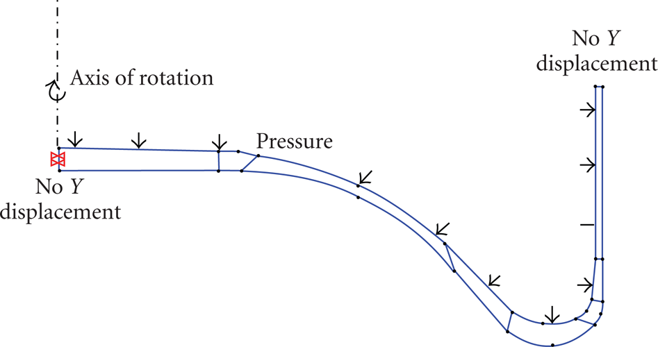
Using the finite element model shown in Figure 9, made up of 5165 six-noded three-dimensional wedge elements and generated automatically from the cross-section shown in Figure 8, finite element predictions of yield and elastic-plastic buckling pressures of 1.20 and 1.53 MPa, respectively, were predicted. Unlike the axisymmetric model, this model is able to resist a further increase in pressure, prior to collapse and the predicted collapse pressure (above which convergence was not achieved) is 2.02 MPa. The predicted elastic-plastic buckling mode, at a pressure of 1.53 MPa, is shown in Figure 10. Again, due to the tolerance on the convergence criteria, equivalent stresses of up to 7% higher than the yield stress are predicted. The predicted shape is very similar to that seen in experimental burst testing, for which a typical failure is shown in Figure 11. This will be reported in a later paper.

Figure 9:

Three-dimensional finite element model for can with variable thickness.

Figure 10:

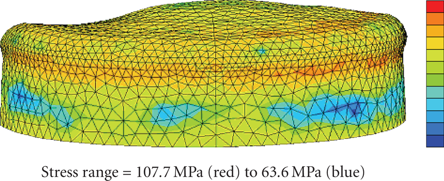
Elastic-plastic buckling equivalent stress contour plot for variable thickness model at p=1.53 MPa.

Figure 11:

Burst aerosol can showing the elastic-plastic buckling mode.

5. Discussion of Results

The application of the elastic compensation method to upper and lower bound calculations is relatively straight-forward. However, it is an iterative, time-consuming process and so a simple FORTRAN user interface with the finite element program has been developed in order to automatically modify the values of Young's modulus for each element after each iteration and to monitor convergence. The upper bound estimate is then easily evaluated from the converged solution. The lower bound estimate, however, also requires the strain energy and dissipation energy for the converged solution. Whereas some finite element programs provide details of strain energy, the dissipation energy may not be readily available and a further FORTRAN program to obtain this value from the finite element predictions of principal strains has been developed.

The paper presents an interesting deviation from the usual application of the elastic compensation method. It is recognized that elastic-plastic buckling problems of this type, involving large displacements, are not strictly suited to analysis via the elastic compensation method, which is based on small strain theory. This is particularly true for the geometrically nonlinear collapse mechanism associated with dome reversal. However, the results suggest that there is some merit in carrying out such an analysis to provide an approximate solution at the early design stage and provides additional confidence in the method.

5.1. Constant Thickness Axisymmetric Models

The results presented in Figure 7 show that the predicted collapse pressures lie between the upper and lower bound estimates and this provides a degree of confidence in these approximate methods. However, the range between the upper bound and lower bound is rather large (in the worst case, +71% to − 40% of the predicted collapse pressure). Furthermore, the lower bound is always greater than the yield stress. This limits the use of these approximate methods for this type of geometry and loading to collapse pressure estimates. Nevertheless, the elastic compensation method is useful since it only requires elastic analyses.

Although axisymmetric models can provide some useful information on the elastic and elastic-plastic behavior of such components under internal pressure, the practical issue of dome reversal cannot be investigated and a full three-dimensional analysis is necessary.

5.2. Variable Thickness Models

A variable thickness model, which reflects the true thickness profile of measured cans, has been used and it is clear that there is a significant difference between the thickness of the cylindrical section (0.32 mm minimum) and that of the base (1.31 mm maximum). In this case, although the axisymmetric model can be used in the elastic compensation method, a full three-dimensional model was used to predict elastic-plastic buckling and plastic collapse.

Again, the upper pressure bound estimate of 2.59 MPa is 28% higher than the predicted plastic collapse pressure of 2.02 MPa, which further demonstrates the usefulness of the elastic compensation method. However, the lower bound estimate of 0.81 MPa is 33% lower than the yield pressure of 1.20 MPa, in a similar way to the predictions for the constant thickness models.

By comparing variable thickness results with those for constant thickness models, it is apparent that the upper and lower bound estimates for the variable thickness model fall between the 0.8 to 1.2 mm constant thickness results, which might be considered to be reasonable since the region with the highest stress concentration and where buckling ultimately occurs (i.e., the discontinuity between cylinder and base) has a thickness varying between 0.7 and 1.3 mm.

6. Conclusions

(1) In all the cases considered, the elastic-plastic predictions of plastic collapse pressure fall within the upper and lower bound estimates and so the upper bound approach, which is far less time-consuming and has less computational complexity, provides a useful estimate of collapse pressure. On the other hand, the lower bound estimate cannot be used safely when “design to avoid yielding” is the criterion. It is suggested that this is due to the complexity of the profile and the resulting nonuniform stress distribution.

(2) The elastic compensation method provides a straight-forward and useful approach, without the need for complex elastic-plastic analysis, which requires knowledge and modeling of the post-yield nonlinear material behavior.

(3) Whereas the lower bound limit load can be obtained directly from the converged elastic solution, additional programming may be needed for the upper bound method in order to calculate dissipation energy from the finite element predictions.

(4) The true thickness profile of a can is far from constant and a direct function of the extrusion process and tooling geometry. Experimental measurements suggest a minimum thickness in the cylindrical section of ≾0.32 mm and a maximum base thickness of ≾1.31 mm. Although the constant thickness models have provided a useful insight into the mechanisms of failure and the usefulness of the elastic compensation method, accurate predictions can only be achieved using a variable thickness model.

(5) The axisymmetric models and three-dimensional models with rotational symmetry can be used to predict initial yield and plastic collapse pressures. However, they are unable to differentiate between elastic-plastic buckling (or dome reversal) and total collapse. For this reason, Robotham et al.'s method [20] of introducing slight geometric imperfections has been used successfully to identify dome reversal.

Footnotes

Notations

Subscripts

Superscripts

References

BS5500, “Specification for Unfired Fusion Welded Pressure Vessels,” British Standards Institution, London, UK, 1997.

ASME Boiler and Pressure Vessel Code, Section VIII, Division 1, “Pressure Vessels,” American Society of Mechanical Engineers, New York, NY, USA, 1995.

Drucker

D. C.

Prager

, and Greenberg

N. J.

, “Extended limit design theorems for continuous media,” Quarterly of Applied Mathematics, vol. 9, no. 4, pp. 381–389, 1952.

Hill

, “On the state of stress in a plastic-rigid body at the yield point,” Philosophical Magazine, vol. 42, no. 7, pp. 868–875, 1951.

Koiter

W. T.

, “General theorems for elastic-plastic solids,” in Progress in Solids Mechanics, Sneddon

I. N.

and Hill

, Eds., pp. 165–221, North-Holland, Amsterdam, The Netherlands, 1963.

Mendelson

, Plasticity: Theory and Application, Macmillan, London, UK, 1968.

Berak

E. G.

and Gerdeen

J. C.

, “A finite element technique for limit analysis of structures,” Journal of Pressure Vessel Technology, vol. 112, no. 2, pp. 138–144, 1990.

Dhalla

A. K.

, “Verification of an elastic procedure to estimate follow-up,” in Design of Elevated Temperature Piping, Mallet

R. H.

and Mello

R. M.

, Eds., pp. 81–96, American Society of Mechanical Engineers, New York, NY, USA, 1984.

Marriott

D. L.

, “Evaluation of deformation or load control of stresses under inelastic conditions using elastic finite element stress analysis,” in Proceedings of the ASME Pressure Vessel and Piping Conference (PVP ′88), vol. 136, pp. 3–9, Pittsburgh, Pa, USA, June 1988.

10.

Mackenzie

and Boyle

J. T.

, “A method of estimating limit loads by iterative elastic analysis—I: simple examples,” International Journal of Pressure Vessels and Piping, vol. 53, no. 1, pp. 77–95, 1992.

11.

Mackenzie

Nadarajah

Shi

, and Boyle

J. T.

, “Simple bounds on limit loads by elastic finite element analysis,” Journal of Pressure Vessel Technology, vol. 115, no. 1, pp. 27–31, 1993.

12.

Gowhari-Anaraki

A. R.

and Adibi-Asl

, “Estimation of upper and lower bound limit loads and shakedown load for structural frames based on reduced modulus approach,” in Proceedings of the 6th International Conference on Civil Engineering (ICCE ′03), pp. 399–406, Isfahan, Iran, May 2003.

13.

Hardy

S. J.

Gowhari-Anaraki

A. R.

, and Pipelzadeh

M. K.

, “Upper and lower bound limit and shakedown loads for hollow tubes with axisymmetric internal projections under axial loading,” Journal of Strain Analysis for Engineering Design, vol. 36, no. 6, pp. 595–604, 2001.

14.

Pham

D. C.

, “Shakedown kinematic theorem for elastic-perfectly plastic bodies,” International Journal of Plasticity, vol. 17, no. 5, pp. 773–780, 2001.

15.

Weichert

and Hachemi

, “Influence of geometrical nonlinearities on the shakedown of damaged structures,” International Journal of Plasticity, vol. 14, no. 9, pp. 891–907, 1998.

16.

Seshadri

and Kizhatil

R. K.

, “Inelastic analyses of pressure components using the ‘GLOSS’ diagram,” in Proceedings of the ASME Pressure Vessels and Piping Conference (PVP ′90), vol. 186, pp. 105–113, Nashville, Tenn, USA, June 1990.

17.

Calladine

C. R.

, Plasticity for Engineers, Ellis Horwood, Chichester, UK, 1985.

18.

“ELFEN User Manual Version 3.0,” Rockfield Software, Swansea, UK, 2001.

19.

Hardy

S. J.

and Abdusslam

, “Finite element modelling of the manufacturing process for aluminium aerosol cans,” Proceedings of the Institution of Mechanical Engineers, Part L: Journal of Materials: Design and Applications, vol. 221, no. 4, pp. 265–274, 2007.

20.

Robotham

W. S.

Hyde

T. H.

Williams

E. J.

, and Taylor

J. W.

, “Elastic-plastic buckling behaviour of shafts in torsion,” The Aeronautical Journal, vol. 104, no. 1031, pp. 1–7, 2000.