Optimal capacity sizing of park‐and‐ride lots with information‐aware commuters

Abstract

We study capacity sizing of park‐and‐ride lots that offer services to commuters sensitive to congestion and parking availability information. The goal is to determine parking lot capacities that maximize the total social welfare for commuters whose parking lot choices are predicted using the multinomial logit model. We formulate the problem as a nonconvex nonlinear program that involves a lower and an upper bound on each lot's capacity, and a fixed‐point constraint reflecting the effects of parking information and congestion on commuters' lot choices. We show that except for at most one lot, the optimal capacity of each lot takes one of three possible values. Based on analytical results, we develop a one‐variable search algorithm to solve the model. We learn from numerical results that the optimal capacity of a lot with a high intrinsic utility tends to be equal to the upper bound. By contrast, a lot with a low or moderate‐sized intrinsic utility tends to attain an optimal capacity on its effective lower bound. We evaluate the performance of the optimal solution under different choice scenarios of commuters who are shared with real‐time parking information. We learn that commuters are better off in an average choice scenario when both the effects of parking information and congestion are considered in the model than when either effect is ignored from the model.

INTRODUCTION

Park and ride has become an indispensable part of life for many people who commute between their homes in suburban areas and workplaces in central business districts (CBDs). A park‐and‐ride lot (or simply, a lot) is a key facility in a park‐and‐ride system where commuters can park their cars and get access to public transit. Park‐and‐ride lots are designed, maintained, and managed by state or local departments of transportation (DOTs) to serve communities in the satellite cities of a core urban area. For example, there are 134 park‐and‐ride lots with around 22,453 spaces scattered in the satellite cities surrounding the Seattle CBD (WSDOT, 2022). Table 1 shows example park‐and‐ride lots, their capacities, and average daily utilization in 2021 (PSRC, 2022).

TABLE 1

The spaces and utilization of example park‐and‐ride lots in the Greater Seattle Area in 2021.

Park and ride name	Address	Capacity	Utilization
Arlington P&R	SR 9 & SR 530	25	36%
Smokey Point Community Church	SmokeyPt Blvd/77th St NE	50	24%
All Saints Lutheran Church	27225 Military Rd S	75	46%

Park and ride in the United States can date back to the 1930s (Noel, 1988) and received great attention in the 1970s when the DOTs in different urban areas attempted to introduce an economical travel mode as an alternative to driving private cars all the way to office, in response to growing oil prices brought about by the Oil Crisis (Spillar, 1997). As green mobility attracts the growing attention of policymakers, recent years have witnessed an increasing interest in park and ride that is believed to reduce traffic jams and emissions (Holgúin‐Veras et al., 2012; Stieffenhofer et al., 2016).

This work investigates the optimal capacity sizing problem for a park‐and‐ride system, in which a DOT plans to design or redesign a set of park‐and‐ride lots in a specific service area, for example, a satellite city, and needs to determine the optimal capacity of each lot. The capacities of all the lots form a vector called a capacity plan. The ridership demand model that forecasts the demand at a lot plays a central role in the problem. The demand is interchangeably used with the traffic flow routed through the lot in this paper and measured as the number of commuter vehicles parked at the lot during a period of time (e.g., peak hours on weekday mornings) in practice. The number of park‐and‐ride commuters per parked vehicle is often estimated according to the experience of practitioners and historical data. For instance, the number is estimated to be 1.4 in Bullard and Christiansen (1983). Without loss of generality (w.l.o.g.), we assume that one parked vehicle is occupied by one commuter.

A ridership demand model is expected to possess several basic features. First, the demands at all lots within the same service area are interdependent, since they serve the same group of commuters. Second, the demands are influenced by the DOT's capacity sizing decision. To elaborate, the capacities of the lots will affect the parking utilization that will be shared with commuters (cf. Table 1), and therefore affect the attractiveness of each lot to the commuters who are aware of (and sensitive to) the information. As a result, the capacity sizing decision may affect the likelihood of commuters choosing to visit a particular lot, thus affecting the demands. Third, the congestion effect should be captured by the demand model. The congestion effect refers to the phenomenon that the utility of a service or facility erodes as it serves a higher demand. Given a capacity sizing decision, the utility of a lot perceived by commuters, which represents the preference of commuters toward the lot, drops as more commuters choose to use the lot due to the congestion effect and increasing parking utilization. Observe that the park‐and‐ride demands depend on the utilities of the lots, which are, in turn, affected by the demands. This relation may lead to the well‐known phenomenon called traffic equilibrium, which has been observed in queueing systems (Maglaras et al., 2018), seaport operation systems (Wang & Meng, 2019), and transportation systems (Cascetta, 2009). Discrete choice models, such as the multinomial logit (MNL) model, nested logit (NL) model, and mixed logit (ML) model (Ben‐Akiva & Lerman, 1985; Train, 2009), have been broadly used to model the choice behavior of travelers facing a set of transportation modes such as riding public transit and driving a private car (Holgúin‐Veras et al., 2012; Naumov et al., 2020).

We will model the ridership demand at a lot using an MNL‐based commuter choice model. The commuter choice model forecasts the probability of commuters choosing a lot based on the utilities of all the lots, thus reflecting the interdependence among the demands at all the lots. A lot's utility is first affected by a variety of physical attributes such as the lot's economic attraction, accessibility, and the transit fare. This part of the utility is called the intrinsic utility. Meanwhile, the utility is formulated to depend on the demand and (average) parking utilization to account for the effects of congestion and parking information on commuter choice. The commuter choice model developed in this work can be viewed as an extended version of the site‐level demand model, which has been applied to forecast the demands for individual park‐and‐ride lots (Abdus‐Samad & Grecco, 1972; Bullard & Christiansen, 1983; Niles & Pogodzinski, 2021; Spillar, 1997). Using the MNL‐based commuter choice model, we represent the demands at all lots at equilibrium (given a capacity sizing decision) as a solution to a (vector) fixed‐point equation.

Next, we explain the objective value and various constraints in the problem. As explained in Litman (2019), one of the primary goals of public transit is to achieve social welfare benefits. The total social welfare can be interpreted as the overall satisfaction received by all park‐and‐ride commuters, where the satisfaction of a commuter can be measured by the utility of the park‐and‐ride lot that the commuter chooses to use. As a policymaker, the DOT intends to maximize the total social welfare when sizing a set of park‐and‐ride lots. Meanwhile, the demand realized at each lot cannot exceed the lot's capacity, which is referred to as a capacity constraint. Also, the demands at all lots need to satisfy the fixed‐point equation, which is referred to as the fixed‐point constraint. Besides, as explained in Bullard and Christiansen (1983), there are often constraints on both the minimum and maximum lot sizes due to design and operational features of park‐and‐ride services. For example, a lot should be designed with a minimum size to ensure that it can at least accommodate the demand arriving between two consecutive buses during the morning commute, which we refer to as a lower bound constraint. Meanwhile, there is always an upper bound on the capacity due to limited space and budget, which is referred to as an upper bound constraint. Both the lower and upper bound constraints are called bound constraints.

The objective and contributions

This section describes our objective and contributions. Since we now live in the era of smartphones, it is easier than ever for commuters to access parking availability information through mobile apps or websites. However, the effect of parking information on the travel mode choice of commuters has not been well addressed in the literature on park‐and‐ride capacity sizing.

This work is aimed at bridging the gap by studying optimal capacity sizing of park‐and‐ride lots with consideration of information‐aware commuters. The problem will be formulated as an optimization model, in which we intend to determine an optimal capacity plan for a set of park‐and‐ride lots in a specific service area to maximize the total social welfare received by commuters while honoring the capacity constraints, lower and upper bound constraints, and the fixed‐point constraint.

The main objective of this work is threefold: (i) to characterize the optimal capacities of the lots, (ii) to develop effective algorithms to determine optimal capacities by leveraging the characterization results, and (iii) to provide managerial insights into the properties of optimal capacities and the value of modeling the effects of parking information and congestion in park‐and‐ride capacity sizing.

This work makes the following theoretical contributions:

• (a)

We formulate the optimal capacity sizing problem as a nonconvex nonlinear optimization model with capacity and bound constraints as well as the fixed‐point constraint reflecting the effect of parking information on commuter choice. The problem is challenging to solve due to these constraints. To resolve the challenge, we transform the model into an equivalent flow‐based model, in which the optimal traffic flow rather than capacity is determined for each lot and the fixed‐point constraint is dropped. To the best of our knowledge, this work is the first to model the effect of parking information in park‐and‐ride capacity sizing, which extends the existing literature by adding a novel model and opens doors for future studies on park and ride with information‐aware commuters.

(b)

We show that the flow‐based model is equivalent to a univariate optimization model with only one decision variable (i.e., the total traffic flow through all lots). The univariate model is built upon a subproblem in which the capacity, bound, and fixed‐point constraints are reformulated as constraints over intervals. The subproblem is tractable to analyze due to its simple form of constraints, which paves the way for obtaining analytical results for the capacity sizing problem.

(c)

We provide analytical results that characterize the structure of the optimal solution to the subproblem. Based on the structural results, we characterize the capacity plan that solves the optimal capacity sizing problem.

(d)

We develop a one‐variable search algorithm to determine a near‐optimal capacity plan by leveraging the characterization results. The algorithm involves an efficient solution procedure to determine the traffic flow pattern at equilibrium under any given capacity plan. The procedure is not only useful in sizing park‐and‐ride lots, but also provides traffic engineers with a method to forecast equilibrium traffic flows under the MNL model.

We provide numerical results by solving the optimal capacity sizing problem for the park‐and‐ride lots in the city of Bellevue in Washington State. The numerical analysis serves two purposes: to obtain insights into park‐and‐ride lot design in a satellite city such as Bellevue and to investigate the value of modeling the effects of congestion and parking information in sizing park‐and‐ride lots.

We obtain the following managerial insights from the theoretical and numerical results:

• (1)

The optimal capacity sizing model may be infeasible, which signals the need to adopt smaller lower bounds and/or larger upper bounds on the lots' capacities. When the problem is feasible, except for at most one lot whose optimal capacity is strictly between the lower and upper bounds, the optimal capacity of each lot is equal to one of three values: the lower bound, the upper bound, and the traffic flow through the lot.

(2)

We learn from numerical results that a lot with a high intrinsic utility tends to have its optimal capacity equal to the upper bound. A lot with a low intrinsic utility and a small lower bound tends to have the optimal capacity equal to the optimal traffic flow through the lot, leading to full utilization of the lot. However, when the lower bound is not small, the optimal capacity tends to be equal to the lower bound. We also observe that the parking availability at a lot with full utilization may not be improved by allowing for a smaller lower bound and/or a larger upper bound on the lot's capacity.

(3)

When a lot has a high initial utilization rate, its utilization seems to be nonincreasing as commuters become more sensitive to parking availability. However, if a lot attains low utilization with commuters weakly sensitive to parking availability, the utilization tends to be nondecreasing with possible jumps to lower levels as commuters care more about parking availability.

(4)

Opening a subset of the potential park‐and‐ride lots may yield a higher total social welfare than utilizing all of the available lots.

It is worth noting that the methods developed in this work are not only applicable when a DOT needs to size park‐and‐ride lots from the scratch, but also useful when the DOT needs to redesign or upgrade park‐and‐ride lots, for example, add parking spots with charging stations for electric cars.

The outline of the work

The remainder of the paper is organized as follows. Section 2 reviews the related literature. Section 3 formally defines the optimal capacity sizing problem. In Section 4, we formulate the problem as a nonconvex nonlinear program and transform it into an equivalent flow‐based model. We then pass on to Section 5 to reformulate the flow‐based model as a one‐variable optimization model. Section 6 presents a search algorithm to solve the problem. Numerical studies are provided in Section 7 and conclusions are drawn in Section 8. Supplement materials and all the proofs are provided in the Supporting Information.

LITERATURE REVIEW

There are two streams of research related to our work: park‐and‐ride capacity sizing and multiproduct price optimization under customer choice, which are discussed in Sections 2.1 and 2.2, respectively.

Capacity sizing for park‐and‐ride lots

This work follows the line of research on capacity sizing for park‐and‐ride lots. Early studies, such as Abdus‐Samad and Grecco (1972) and Spillar (1997), were mostly performed in collaboration with local DOTs and focused on developing site‐level demand models, in which regression analysis is applied to forecast the demand at an individual park‐and‐ride lot based on characteristics such as the location and accessibility. These studies treat demand forecasting and capacity sizing as two separate decision‐making processes: Demand is estimated first and a capacity size is then chosen to serve the anticipated demand. This two‐step method suffers from two drawbacks. First, the method results in an independent‐demand model (Talluri & van Ryzin, 2004): The demand at a lot is not influenced by capacity sizing decisions, which is not necessarily true in practice. Second, the demand is estimated for a single lot and does not depend on the demands at all other lots, which may be unrealistic when multiple lots serve the same area and are thus regarded as substitutable or interchangeable by commuters. Nordstrom and Christiansen (1981) and Bullard and Christiansen (1983) applied site‐level models to estimate park‐and‐ride demands in Texas based on nonlinear regression that uses parking capacity as one of the predictor variables. They use a presumed capacity size for demand forecasting, which may, however, result in a forecasted demand violating the capacity constraint. In a recent study, Niles and Pogodzinski (2021) developed ridership demand models for individual park‐and‐ride lots in San José, Seattle, and Los Angeles using regression.

Region‐level demand models have also been employed by researchers, such as Hendricks and Outwater (1998), Spillar (1997), and Holgúin‐Veras et al. (2012), to forecast park‐and‐ride demands. In these models, the flows routed through different paths/travel modes between each pair of origin and destination zones over a study area are estimated and the park‐and‐ride demands are then calculated based on the flows. Nonetheless, site‐level demand models have continued to receive attention from practitioners for two reasons. First, a site‐level demand model is often more effective in providing accurate site‐specific forecasts, while a region‐level model tends to overestimate park‐and‐ride demands, particularly when the travel characteristics incorporated into the model do not correspond to the realized design and construction conditions of the park‐and‐ride lots (Spillar, 1997). Second, a site‐level model often requires a smaller amount of data to estimate than a region‐level model, thus particularly favored by practitioners with limited data and computational resources. The commuter choice model developed in this work can be thought of as an improved site‐level demand model, by which the forecasted park‐and‐ride demands are interdependent across all the lots in the same service area and dependent on capacity sizing decisions.

The literature on addressing demand forecasting and capacity sizing for park‐and‐ride lots under a unified optimization model is limited. For instance, García and Marín (2002) formulated a joint capacity sizing and pricing problem for park‐and‐ride lots as a bilevel programming model, which involves an NL model to describe the travel mode choice of travelers. Song et al. (2017) solved the optimal location problem for park‐and‐ride lots by determining the optimal capacities and frequencies of transit services at the lots. The problem was formulated as a mathematical program with equilibrium constraints under an MNL model. Liu et al. (2018) studied optimal capacity sizing for the park‐and‐ride facilities in a suburban area and formulated the problem as a mathematical program with equilibrium constraints, where a crossed‐NL model is used to describe the choice behavior of travelers. Henry et al. (2022) investigated the park‐and‐ride facility location problem for an on‐demand transportation system and used an MNL model to forecast commuters' choice. Rezaei et al. (2022) studied the optimal park‐and‐ride facility location for Nashville, Tennessee, using a mixed‐integer linear program integrated with an MNL‐based demand model. Readers are referred to Haque et al. (2021) for more literature on park and ride.

Our work sets itself apart from these studies in two major aspects. First, these studies do not address the impact of parking availability information on commuter choice. Second, their studies are focused on developing numerical solutions to find a (local or global) optimal solution, while our work aims to obtain analytical results that characterize the global optimal solution and gain insights from the numerical results. There is another body of literature that discusses the impact of parking information provision on parking policies, such as Qian and Rajagopal (2014) and Jakob et al. (2020). However, these studies focus on a different topic, namely, optimal parking pricing without congestion.

Multiproduct price optimization under customer choice

This work is also related to the literature on multiproduct price optimization under customer choice, particularly on the methodological side. For the sake of comparison, loosely speaking, a park‐and‐ride lot in this work corresponds to a product in multiproduct pricing, the traffic flow routed through a lot resembles the sales of a product, and the capacity of a lot, like the price, serves as a decision lever to adjust demands.

In this literature, one of the inspiring results is that the objective value function, that is, the total profit of the products, under the MNL model is generally not concave with respect to the price vector, but it turns out to be concave with respect to the market share vector (there exists a one‐to‐one correspondence between the price and market share vectors; Li & Huh, 2011; Song & Xie, 2007). As a result, it has been shown that the optimal markup prices for different products are equal when the price sensitivity parameters are identical for the products under the MNL model (Hopp & Xu, 2005; Li & Huh, 2011).

Efforts have recently been invested in understanding whether or not the same or similar results hold under other choice models. To mention only a few, Gallego and Wang (2014) studied price optimization and competition for multiple products under the NL model with heterogeneous price sensitivity parameters within and across the nests. The authors maintained that the objective value function with respect to the market share vector is not necessarily concave under the NL model. Rayfield et al. (2015) developed approximation methods to solve the multiproduct price and assortment optimization problems under the NL model. A unique feature considered in this work is that there are lower and upper bounds on the prices. Zhang et al. (2018) studied multiproduct price optimization with convex constraints on purchase probabilities under the generalized extreme value models (which include the MNL and NL models as special cases). The authors showed that the optimal markup price is constant across products when the problem is unconstrained and price sensitivities are homogeneous. They also showed that the market‐share–based transformation with constraints is, in fact, a convex program. More examples include Dong et al. (2019) based on Markov choice models and Li (2020) with diffusion‐choice models. However, these works do not involve the fixed‐point constraint, which is critical in the park‐and‐ride capacity sizing problem considered in our work.

Du et al. (2016) are the first to study multiproduct price optimization under the network effect that a product becomes more appealing to consumers as it attracts a larger market share. The problem was formulated as a nonlinear program with a vector fixed‐point equation constraint based on the MNL model. The authors highlighted that the objective value function in the sales‐based (i.e., market‐share–based) transformation is not necessarily convex or concave. The authors obtained an interesting result that the optimal prices can take at most two distinct values even when the intrinsic utilities, network sensitivities, and price sensitivities are identical for different products. In their subsequent work, Du et al. (2018) solved the worst‐case pricing problem for a single product under the network effects. Nosrat et al. (2021) studied optimal pricing for a single product with multiple customer segments and the network effects under a mixture of MNL models. Our work distinguishes itself from this series of works by the following features. First, these studies do not consider bound constraints on sales or prices, while we consider that the traffic flow (corresponding to the sales) at each lot is limited by its capacity and the capacity (corresponding to the price) is bounded from below and above. Second, the utility function of a product is separable in the sales and price, while the utility of a park‐and‐ride lot is nonseparable in the traffic flow and capacity. Third, the utility of a park‐and‐ride lot is nonincreasing in the traffic flow due to the effects of congestion and parking information, while the utility of a product is nondecreasing in the sales due to the network effects in their studies. Fourth, the objective is to maximize the total profit of a firm in their works, while it is to maximize the total social welfare of commuters in our work. Due to all these different features, which are ultimately attributed to the fact that we consider a different application in transportation, the results and proof techniques in these works do not easily carry through. For instance, the first‐order optimality condition that is one of the key proof techniques in these and other existing studies on optimal pricing needs to be revisited with capacity and bound constraints. Therefore, new analysis techniques are needed to tackle the problem considered in our work.

PROBLEM DESCRIPTION

This section describes the optimal capacity sizing problem for park‐and‐ride lots with information‐aware commuters. More specifically, Section 3.1 introduces the notation adopted in this work. In Section 3.2, we develop the MNL‐based commuter choice model with the effects of congestion and parking information. In Section 3.3, we discuss the properties of the traffic flows at equilibrium. We formulate the total social welfare in Section 3.4.

Notation

We use

${\mathbb{R}}_{+}:=[0,\infty )$

to denote the set of nonnegative real numbers and

${\mathbb{R}}_{++}:=(0,\infty )$

to represent the set of positive real numbers. Let [n] denote the integer set

$[n]:=\{1,2,\text{…},n\}$

for any

$n\in \mathbb{N}$

. For any

$\mathbf{x}\in {\mathbb{R}}^n$

, where

$n\in \mathbb{N}$

, let

$\mathrm{diag}(\mathbf{x})$

denote the

$n\times n$

diagonal matrix generated from

$\mathbf{x}$

such that

$x_i$

is the i‐th diagonal entry for each

$i\in [n]$

and all other entries are zeros. Let

$\mathbf{e}\in {\mathbb{R}}^J$

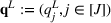
denote a J‐dimensional vector with all entries equal to one. All vectors are column vectors unless otherwise specified. However, for the economical use of space, we write

$\mathbf{x}=(x_1,x_2,\text{…},x_n)$

inside of the text to describe entries of vector

$\mathbf{x}\in {\mathbb{R}}^n$

. In addition, we conform to the convention that

$1/\infty =0$

,

$\log (0)=-\infty$

, and

$a+\infty =\infty$

for all

$a\in \mathbb{R}$

and that any set

$\{m,m+1,\text{…},n\}$

is empty if

$m>n$

for any

$m,n\in \mathbb{Z}$

. Let

$\mathbf{1}\{A\}$

denote the indicator function for any event A and

${\parallel ·\parallel }_1$

denote the 1‐norm. Define

$x\vee y:=\max \{x,y\}$

and

$x\wedge y:=\min \{x,y\}$

for all

$x,y\in \mathbb{R}$

. Let

$|A|$

denote the cardinality of any discrete set A.

Commuter choice model with congestion and parking information

In this section, we formulate the commuter choice model with congestion and parking effects.

Consider a population of commuters who travel on workdays from their homes within a service area (e.g., a satellite city) to their work sites in an urban CBD. There exists a set [J] of park‐and‐ride lots available to the commuters in the service area, where

$J\in \mathbb{N}$

. For each

$j\in [J]$

, let

$q_j\in {\mathbb{R}}_{+}$

denote the (average) traffic flow attracted by j during a given time period, for example, the morning commute between 7 a.m. and 9 a.m. on workdays. Define

$\mathbf{q}:=(q_j,j\in [J])$

as the vector of flows for all the lots, which is referred to as the flow pattern. Let

$C_j\in [0,\infty ]$

denote the capacity of the lot j and define

$\mathbf{C}:=(C_1,C_2,\text{…},C_J)$

as the vector of capacities, which is referred to as the capacity plan. Let

${\ell }_j\in {\mathbb{R}}_{++}$

denote the lower bound on the capacity

$C_j$

and

$u_j\in {\mathbb{R}}_{++}$

denote the upper bound on

$C_j$

, where

${\ell }_j<u_j$

. The lower bound represents the minimum design capacity to meet operations constraints, such as the minimum number of commuters to be served during the time headway between two consecutive transit services and the upper bound is due to constraints such as space and budget limits.

Let

$U_j(q_j,C_j)$

denote the utility of any

$j\in [J]$

perceived by commuters, which is expressed as a random variable consisting of two components as follows:

$$U_j(q_j,C_j)={\nu }_j(q_j,C_j)+{\epsilon }_j,$$

1

where

${\nu }_j(q_j,C_j)$

is the systematic utility and

${\epsilon }_j$

is the random error reflecting the variation in the preferences of commuters toward j. The systematic utility is a function of

$q_j$

and

$C_j$

defined as

$${\nu }_j(q_j,C_j)=b_j-\beta q_j^{\theta }+\phi \left(1-q_j/C_j\right).$$

2

The first term

$b_j\in \mathbb{R}$

represents the intrinsic utility of the park‐and‐ride lot j, which measures the attractiveness of j due to characteristics such as accessibility, location, reputation, and transit fares. The second term is similar in form to the widely used Bureau of Public Roads (BPR) function in urban transportation (Sheffi, 1985), which reflects the congestion effect. As in the BPR function,

$\theta \in {\mathbb{R}}_{+}$

is a parameter to be estimated from data and

$\beta \in {\mathbb{R}}_{+}$

is the congestion sensitivity parameter. The third term captures the effect of parking information, in which

$q_j/C_j$

is the utilization of the lot j shared with commuters such as those in Table 1,

$(1-q_j/C_j)$

is the corresponding parking availability at j, and

$\phi \in {\mathbb{R}}_{+}$

is the parking sensitivity parameter, which is assumed to be nonnegative to reflect that commuters appreciate a lot better if it has more availability. Define

$\mathit{\nu }(\mathbf{q},\mathbf{C}):=({\nu }_j(q_j,C_j),j\in [J])$

as the vector of utilities for all the park‐and‐ride lots.

Let

$Q\in {\mathbb{R}}_{++}$

denote the total travel demand originating from the service area during the given time period. Then, we have

$Q={\sum }_{j=0}^J{q}_j$

, where

$q_0\in [0,Q]$

denotes the number of commuters choosing not to park and ride, such as those driving private cars to office. Let

$j=0$

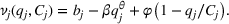
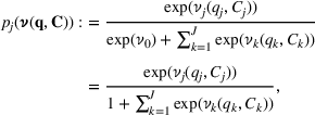
denote the no‐park‐and‐ride alternative representing the choice of commuters not to park and ride at any lot in [J]. Let ν₀ and ε₀ denote the systematic utility and random error of the no‐park‐and‐ride alternative, respectively.

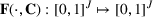
Define

$p_j:{\mathbb{R}}^J\mapsto [0,1]$

as a choice function mapping from

$\mathit{\nu }(\mathbf{q},\mathbf{C})$

to the probability of commuters choosing the park‐and‐ride lot j from the set [J]. We assume that each commuter is a utility maximizer who will choose the alternative with the largest utility among from [J]. We also assume that the random errors

${\{{\epsilon }_j\}}_{j=0}^J$

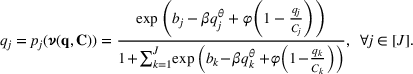
are independent and identically distributed Gumbel random variables with a location parameter 0 and scale parameter 1. Then, according to the random utility theory (Ben‐Akiva & Lerman, 1985), we have

3

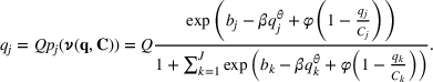
where ν₀ is normalized to zero. It follows from the traffic equilibrium principle (Cascetta, 2009) that the traffic flow through j at equilibrium satisfies

$$\begin{array}{c}\hfill q_j=Q{p}_j(\mathit{\nu }(\mathbf{q},\mathbf{C}))=Q\frac{\exp \left(b_j-\beta q_j^{\theta }+\phi \left(1-\frac{q_j}{C_j}\right)\right)}{1+{\sum }_{k=1}^J\exp \left(b_k-\beta q_k^{\theta }+\phi \left(1-\frac{q_k}{C_k}\right)\right)}.\end{array}$$

Note that we can assume, w.l.o.g., that

$Q=1$

; otherwise, by setting

${\beta }^{\prime }:=\beta Q^{\theta }$

and

$q_k^{\prime }:=q_k/Q$

and

$C_k^{\prime }:=C_k/Q$

for all

$k\in [J]$

, the above equation is equivalent to

$q_j^{\prime }=p_j(\mathit{\nu }({\mathbf{q}}^{\prime },{\mathbf{C}}^{\prime }))$

with β replaced by

${\beta }^{\prime }$

, where

${\mathbf{q}}^{\prime }:=(q_j^{\prime },j\in [J])$

and

${\mathbf{C}}^{\prime }:=(C_j^{\prime },j\in [J])$

. Thus, it follows that

$\mathbf{q}$

satisfies the following vector fixed‐point equation,

$$\begin{array}{c}\hfill q_j=p_j(\mathit{\nu }(\mathbf{q},\mathbf{C}))=\frac{\exp \left(b_j-\beta q_j^{\theta }+\phi \left(1-\frac{q_j}{C_j}\right)\right)}{1+{\sum }_{k=1}^J\exp \left(b_k-\beta q_k^{\theta }+\phi \left(1-\frac{q_k}{C_k}\right)\right)},\forall j\in [J].\end{array}$$

4

Note that

$\mathbf{q}\in {[0,1]}^J$

. Given any capacity plan

$\mathbf{C}\in {(0,\infty ]}^J$

, define a choice operator

$\mathbf{F}(·,\mathbf{C}):{[0,1]}^J\mapsto {[0,1]}^J$

such that

$\mathbf{F}(\mathbf{q},\mathbf{C}):=(p_j(\mathit{\nu }(\mathbf{q},\mathbf{C})),j\in [J])$

for any

$\mathbf{q}\in {[0,1]}^J$

. Then, (4) can be written in a vector form:

$$\mathbf{q}=\mathbf{F}(\mathbf{q},\mathbf{C}).$$

5

Properties of the equilibrium flow pattern

In this section, we discuss the properties of the solution to the fixed‐point equation (5), which will be useful in later sections.

Remark 1 shows the existence and uniqueness of the solution to (5) for any given capacity plan. Remark 1

Consider any

$\mathbf{C}\in {(0,\infty ]}^J$

. Since

$\mathbf{F}(·,\mathbf{C})$

is a continuous function defined in the set [0, 1] ^J , [0, 1] ^J is a nonempty compact and convex set, and the range

$\mathbf{F}({[0,1]}^J,\mathbf{C})\subset {[0,1]}^J$

, it follows from the Brouwer's fixed‐point theorem in section A.3.1 of Cascetta (2009) that there exists a solution to (5). Moreover, since

${\nu }_j$

is strictly decreasing in

$q_j$

for each

$j\in [J]$

, it follows from Cascetta (2009, pp. 311–312) that the solution to (5) is unique.

Define

$\mathcal{Q}:=\{\mathbf{q}\in {[0,1]}^J:q_j>0\forall j\in [J],\parallel \mathbf{q}{\parallel }_1<1\}$

. Remark 2 provides an alternative form of the fixed‐point equation and shows that any equilibrium flow pattern is in

$\mathcal{Q}$

. Remark 2

The fixed‐point equation (4) (and (5)) is equivalent to:

$\log (q_j)={\log (1-\parallel \mathbf{q}\parallel }_1)+b_j-\beta q_j^{\theta }+\phi (1-q_j/C_j)$

for all

$j\in [J]$

. For any

$\mathbf{C}\in {(0,\infty ]}^J$

, if

$\mathbf{q}=\mathbf{F}(\mathbf{q},\mathbf{C})$

, then

$\mathbf{q}\in \mathcal{Q}$

.

Proposition 1 characterizes the monotonicity of the total traffic flow served by all the lots with respect to

$\mathbf{C}$

at equilibrium. Proposition 1

Given capacity plans

${\mathbf{C}}^1,{\mathbf{C}}^2\in {(0,\infty ]}^J$

, let

${\mathbf{q}}^i:=(q_j^i,j\in [J])$

be the flow pattern such that

${\mathbf{q}}^i=\mathbf{F}({\mathbf{q}}^i,{\mathbf{C}}^i)$

for

$i\in \{1,2\}$

. If

${\mathbf{C}}^1\le {\mathbf{C}}^2$

(component‐wisely), then

$\parallel {\mathbf{q}}^1{\parallel }_1\le {\parallel {\mathbf{q}}^2\parallel }_1$

.

Proposition 1 states that if we increase or maintain the same capacity for each lot, then the total number of commuters choosing to park and ride will not decrease at equilibrium.

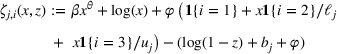
The total social welfare

In this section, we formulate the total social welfare and define the optimal capacity sizing problem.

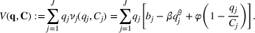
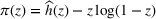
Let

$V(\mathbf{q},\mathbf{C})$

denote the total social welfare, which is the sum of the systematic utilities received by all commuters, namely,

$$\begin{array}{c}\hfill V(\mathbf{q},\mathbf{C}):=\sum _{j=1}^J{q}_j{\nu }_j(q_j,C_j)=\sum _{j=1}^J{q}_j\left[b_j-\beta q_j^{\theta }+\phi \left(1-\frac{q_j}{C_j}\right)\right].\end{array}$$

6

We hereby note that

$V(\mathbf{q},\mathbf{C})$

can be explained as the expected utility that an average commuter would receive upon her arrival at a lot, which is not the same as the

$\mathbb{E}[{\max }_{j\in [J]\cup \{0\}}{U}_j(q_j,C_j)]$

known as the satisfaction of commuters (Sheffi, 1985). The satisfaction can be thought of as the expected perceived utility of a commuter upon departure from home.

When the system reaches equilibrium under a given capacity plan

$\mathbf{C}$

, it follows from Remark 2 that

$b_j-\beta q_j^{\theta }+\phi (1-q_j/C_j)=\log (q_j){-\log (1-\parallel \mathbf{q}\parallel }_1)$

for each

$j\in [J]$

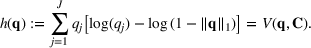
. Substituting it into (6) gives that the total social welfare can also be rewritten as a function

$h:\mathcal{Q}\mapsto \mathbb{R}$

:

$$\begin{array}{c}\hfill h(\mathbf{q}):=\sum _{j=1}^J{q}_j\left[\log (q_j)-\log \left(1-{\parallel \mathbf{q}\parallel }_1\right)\right]=V(\mathbf{q},\mathbf{C}).\end{array}$$

7

Let

$W:[-e^{-1},\infty )\mapsto [-1,\infty )$

denote the principal branch of the Lambert‐W function (Stewart, 2005). Proposition 2 shows that h is strictly convex over

$\mathcal{Q}$

. Proposition 2

h is strictly convex over

$\mathcal{Q}$

and attains a unique minimum over

$\mathcal{Q}$

at

${\mathbf{q}}^{†}=(q^{†},q^{†},\text{…},q^{†})$

, where

$q^{†}:=W(J/e)/[J(W(J/e)+1)]$

. Furthermore,

$h({\mathbf{q}}^{†})=-W(J/e)$

.

We close this section by formally stating the optimal capacity sizing problem for park‐and‐ride lots: The DOT needs to determine the capacity plan that maximizes the total social welfare subject to the capacity and bound constraints as well as the fixed‐point constraint (5).

THE MODELS

In this section, we formulate the optimal capacity sizing problem as optimization models.

The optimal capacity sizing problem can be formulated as the following basic model:

$$\begin{array}{c}\hfill (Basic)\underset{\mathbf{q},\mathbf{C}}{sup}V(\mathbf{q},\mathbf{C})\end{array}$$

8

9

10

11

12

where the objective function value (8) is the total social welfare to be maximized, Constraints (9) ensure that a feasible flow pattern satisfies the fixed‐point equation (5), Constraints (10) set the upper and lower bounds on the capacity of each lot, Constraints (11) ensure that the traffic flow through each lot does not exceed the lot's capacity, and Constraint (12) is the natural constraint. Throughout the remaining paper, let

$({\mathbf{q}}^{\ast },{\mathbf{C}}^{\ast })$

denote an optimal solution to the model (Basic), where

${\mathbf{C}}^{\ast }:=(C_j^{\ast },j\in [J])$

is the optimal capacity plan and

${\mathbf{q}}^{\ast }:=(q_j^{\ast },j\in [J])$

is the equilibrium flow pattern under

${\mathbf{C}}^{\ast }$

.

Next, we reformulate the model (Basic) as an optimization model that has

$q_1,q_2,\text{…},q_J$

rather than

$C_1,C_2,\text{…},C_J$

as decision variables. Define a function

$${\xi }_j(\mathbf{q}):=\frac{\phi q_j}{y_j(\mathbf{q})},$$

13

for all

$\mathbf{q}\in \mathcal{Q}$

, where

$y_j(\mathbf{q}):=b_j+\phi -\beta q_j^{\theta }{+\log (1-\parallel \mathbf{q}\parallel }_1)-\log (q_j)$

for all

$j\in [J]$

. Also define a vector‐valued function

$\mathit{\xi }:=({\xi }_1,{\xi }_2,\text{…}{\xi }_J)$

such that

$\mathit{\xi }(\mathbf{q}):=({\xi }_j(\mathbf{q}),j\in [J])$

for all

$\mathbf{q}\in \mathcal{Q}$

.

Let

$\mathcal{D}:=\{\mathbf{q}\in \mathcal{Q}:\mathit{\xi }(\mathbf{q})\in {\mathbb{R}}_{++}^J\}$

denote the domain of ξ mapping into positive vectors. Some discussions on the function

$\mathit{\xi }(\mathbf{q})$

are provided in Remark 3 and Lemma 1. Remark 3

For every

$\mathbf{q}\in \mathcal{D}$

,

$(\mathbf{q},\mathbf{C})$

satisfies

$\mathbf{q}=\mathbf{F}(\mathbf{q},\mathbf{C})$

if and only if

$\mathbf{C}=\mathit{\xi }(\mathbf{q})$

. Thus,

${\mathbf{C}}^{\ast }=\mathit{\xi }({\mathbf{q}}^{\ast })$

.

Lemma 1 claims that

$\mathit{\xi }:\mathcal{D}:\mapsto {\mathbb{R}}_{++}^J$

is bijective. Lemma 1

ξ is a continuous bijection in

$\mathcal{D}$

and

${\mathit{\xi }}^{-1}:{\mathbb{R}}_{++}^J\mapsto \mathcal{D}$

 exists.

It follows from

$h(\mathbf{q})$

defined in (7) and (9) that the model (Basic) is equivalent to the following flow‐based model, where the primary decision variables are in

$\mathbf{q}=(q_1,q_2,\text{…},q_J)$

:

14

15

16

where

${\xi }_j(\mathbf{q})$

is defined in (13).

Let

$\mathcal{S}:=\{\mathbf{q}\in \mathcal{Q}:\mathit{\xi }(\mathbf{q})\in {\prod }_{j=1}^J[{\ell }_j,u_j],\mathit{\xi }(\mathbf{q})\ge \mathbf{q}\}$

denote the feasible set of the model (Flow). Since

$\mathcal{Q}$

is open, it is not obvious that

$\mathcal{S}$

is open or closed. We need to examine the compactness of

$\mathcal{S}$

to conclude whether or not an optimal solution can be attained in

$\mathcal{S}$

. Proposition 3 guarantees the existence of an optimal solution in

$\mathcal{S}$

when the model (Flow) is feasible, which justifies the use of “max ” instead of “

$sup$

” in the model and is shown based on Lemma 1. Proposition 3

$\mathcal{S}$

is a compact set. If

$\mathcal{S}\ne ⌀$

, then there exists an optimal solution in

$\mathcal{S}$

that solves the model (Flow).

Figure 1 illustrates the feasible set and the objective function

$h(\mathbf{q})$

in the model (Flow) when

$J=2$

,

$\beta =18.929$

,

$\theta =0.923$

,

$\phi =3.301$

,

$b_1=-2.551$

,

$b_2=-3.281$

,

${\ell }_1=0.05$

,

$u_1=0.95$

,

${\ell }_2=0.15$

, and

$u_2=0.85$

. A circle in Figure 1a denotes a feasible flow pattern

$\mathbf{q}=(q_1,q_2)$

and a cube in Figure 1b represents

$h(\mathbf{q})$

at a feasible

$\mathbf{q}$

.

FIGURE 1

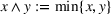
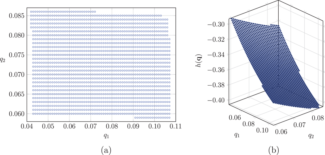
The illustration of the feasible set and objective function in the model (Flow). (a) The feasible set. (b) The objective function.

As illustrated in Figure 1, the feasible set in the model (Flow) is not necessarily convex, which makes the model challenging to solve or analyze. The model is further complicated by the following features. First, the objective function

$h(\mathbf{q})$

is strictly convex (cf. Proposition 2), and therefore, we are confronted with a nonconvex program. Second, the unconstrained first‐order optimality condition, which is one of the key analysis techniques used in the existing literature, may not hold due to the capacity and bound constraints. Third, the model may be infeasible due to these constraints. Thus, it requires a better understanding of the conditions under which the model is feasible.

CHARACTERIZING THE OPTIMAL CAPACITY PLAN

In this section, we characterize the structure of the optimal capacity plan. First, we build in Section 5.1 a univariate model that is equivalent to the model (Flow) but more amenable to analysis. Then, in Section 5.2, we characterize the optimal solution to the subproblem embedded in the univariate model, based on which we obtain characterizations of the optimal capacity plan.

An equivalent univariate model

The model (Flow) is challenging to analyze due to its nonconvexity and constraints. To resolve the challenge, we build in this section a univariate model and show its equivalence to the model (Flow).

Let

$z:={\parallel \mathbf{q}\parallel }_1$

denote the total traffic flow attracted by all lots, where

$q_j$

is the traffic flow through j for any

$j\in [J]$

. Note that

$z={\sum }_{k=1}^J\exp ({\nu }_k(q_k,C_k))/(1+{\sum }_{k=1}^J\exp ({\nu }_k(q_k,C_k)))$

according to the fixed‐point equation (4). By a change of variables, we will transform the model (Flow) with

$q_1,q_2,\text{…},q_J$

as decision variables into a univariate model with z as the only decision variable.

Reformulating Constraints (14)–(16)

First, we reformulate Constraints (14)–(16) as a function of variable z. It can be observed from (13)–(16) that given

$z={\parallel \mathbf{q}\parallel }_1$

, the feasible region of the traffic flow

$q_j$

for any lot

$j\in [J]$

is independent of the traffic flows for all other lots. Hence, these constraints can be represented as the intersection of individual feasible regions of

$q_1,q_2,\text{…},q_J$

.

For

$j\in [J]$

, let

${\mathcal{Q}}_j(z)$

denote the feasible region of

$q_j$

given the total traffic flow

$z\in (0,1)$

. To obtain an explicit expression of

${\mathcal{Q}}_j(z)$

, define a function

${\zeta }_{j,i}(·,z):[0,1]\mapsto [-\infty ,\infty )$

as:

17

for

$i\in \{1,2,3\}$

.

The functions

${\zeta }_{j,i}(x,z)$

for

$i\in \{1,2,3\}$

are used to reformulate the constraints

${\xi }_j(\mathbf{q})\ge q_j$

,

${\xi }_j(\mathbf{q})\ge {\ell }_j$

and

${\xi }_j(\mathbf{q})\le u_j$

in (14)–(16) as

${\zeta }_{j,1}(q_j,z)\ge 0$

,

${\zeta }_{j,2}(q_j,z)\ge 0$

, and

${\zeta }_{j,3}(q_j,z)\le 0$

, respectively, when z is the given total traffic flow. To explain, given z, it follows from (13) that

${\xi }_j(\mathbf{q})\ge q_j$

leads to

$\phi q_j/y_j(\mathbf{q})\ge q_j$

, which is equivalent to

$\phi -y_j(\mathbf{q})=\beta q_j^{\theta }+\log (q_j)-(\log (1-z)+b_j)={\zeta }_{j,1}(q_j,z)\ge 0$

since

$q_j>0$

due to

$\mathbf{q}\in \mathcal{Q}$

. Similarly,

${\xi }_j(\mathbf{q})\ge {\ell }_j$

and

${\xi }_j(\mathbf{q})\le u_j$

can be substituted by

${\zeta }_{j,2}(q_j,z)\ge 0$

and

${\zeta }_{j,3}(q_j,z)\le 0$

, respectively.

Remark 4 provides a description of

${\mathcal{Q}}_j(z)$

based on the explanations above. Remark 4

For any

$z\in (0,1)$

and

$j\in [J]$

, the feasible region

${\mathcal{Q}}_j(z)$

of

$q_j$

specified in (14)–(16) can be represented by

$${\mathcal{Q}}_j(z)=\left\{q_j\in [0,1]:{\zeta }_{j,1}(q_j,z)\ge 0,{\zeta }_{j,2}(q_j,z)\ge 0,{\zeta }_{j,3}(q_j,z)\le 0\right\}.$$

The univariate model

The univariate model is represented as:

where z is the only decision variable and

$\widehat{h}(z)$

is the optimal objective value of the subproblem:

Proposition 4 formally establishes the equivalence between the models (Flow) and (Univar). Proposition 4

Consider any optimal flow pattern

${\mathbf{q}}^{\ast }$

that solves the model (Flow). Define

$z^{\ast }:={\parallel {\mathbf{q}}^{\ast }\parallel }_1$

. Then,

$z^{\ast }$

is optimal to the model (Univar) and

${\mathbf{q}}^{\ast }$

is optimal to the model (Sub) with parameter

$z=z^{\ast }$

. Consider any

$\widehat{z}\in (0,1)$

optimal to the model (Univar) and

$\widehat{\mathbf{q}}$

optimal to the model (Sub) with parameter

$z=\widehat{z}$

. Then,

$\widehat{\mathbf{q}}$

is optimal to the model (Flow).

Proposition 4 have several implications. First, it implies that the model (Univar) is feasible if and only if the model (Flow) is feasible. Second, when both the models are feasible, one can retrieve an optimal solution to the model (Flow) from that to the model (Univar). Third, the structure of the optimal flow pattern that solves the model (Flow) can be understood by studying the optimal solution to the model (Sub).

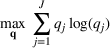
The subproblem

In this section, we characterize the optimal solution to the model (Sub).

Feasibility

First, we discuss the feasibility of the subproblem to gain insights into the feasibility of the model (Univar), which informs of the feasibility of the model (Flow) as indicated by Proposition 4. The feasibility conditions will also be used to develop solution algorithms in Section 6.

Corollary 1 provides a complete characterization of

${\mathcal{Q}}_j(z)$

(i.e., the feasible region of

$q_j$

) for any

$j\in J$

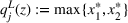
under any given z, which directly follows from Proposition EC.1 in the Supporting Information. Corollary 1

Consider any

$z\in (0,1)$

and

$j\in [J]$

. The following holds:

• (1)

  If

  $\log (1-z)+b_j+\phi >\beta +\phi \min \{1,1/{\ell }_j\}$
  , then
  ${\mathcal{Q}}_j(z)=⌀$
  .

• (2)

  If

  $\log (1-z)+b_j+\phi \le \beta +\phi \min \{1,1/{\ell }_j\}$
  , there exists a unique
  $x_i^{\ast }\in (0,1]$
  such that
  ${\zeta }_{j,i}(x_i^{\ast },z)=0$
  for
  $i\in \{1,2\}$
  . Define the lower bound flow
  $q_j^L(z):=\max \{x_1^{\ast },x_2^{\ast }\}$
  .

Corollary 1 provides conditions for

${\mathcal{Q}}_j(z)=⌀$

and represents

${\mathcal{Q}}_j(z)$

as a simple interval when it is nonempty. If the condition in (1) holds, either

${\zeta }_{j,1}(q_j,z)\ge 0$

or

${\zeta }_{j,2}(q_j,z)\ge 0$

fails to hold, resulting in

${\mathcal{Q}}_j(z)=⌀$

. If the condition in (2)(i) holds but

$x_3^{\ast }>u_j$

, either

${\zeta }_{j,1}(q_j,z)\ge 0$

or

${\zeta }_{j,3}(q_j,z)\le 0$

will be violated, causing

${\mathcal{Q}}_j(z)=⌀$

. Otherwise, there exist a lower bound flow

$q_j^L(z)$

and an upper bound traffic flow

$q_j^H(z)$

such that

${\mathcal{Q}}_j(z)$

can be represented as a nonempty interval

$[q_j^L(z),q_j^H(z)]$

.

Corollary 1 can be used to determine the feasibility of the model (Flow): If

${\mathcal{Q}}_j(z)=⌀$

for some j, then the model (Sub) is infeasible for the given z. Moreover, if the model (Sub) is infeasible for all

$z\in (0,1)$

, both the models (Univar) are (Flow) are infeasible. Also, representing

${\mathcal{Q}}_j(z)$

as intervals allows for obtaining characterization results in Theorem 1. Corollary 1 will also be applied to reduce the search space of z in Algorithm 2.

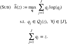
Characterizations of the optimal solution to the subproblem

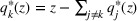
Next, we characterize in Theorem 1 the optimal solution to the model (Sub) using Corollary 1. Theorem 1

Consider any

$z\in (0,1)$

. Assume that

$\log (1-z)+b_j+\phi \le \beta +\phi \min \{1,1/{\ell }_j\}$

for all

$j\in [J]$

and that if there exists

$j\in [J]$

and

$x^{\ast }\in (0,1]$

such that

${\zeta }_{j,3}(x^{\ast },z)=0$

, it holds that

$x^{\ast }\le u_j$

. Let

$q_j^L(z)\in (0,1]$

and

$q_j^H(z)\in (0,1]$

be as in Corollary 1. Then, the model (Sub) is equivalent to

18

19

20

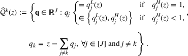
Let

${\mathbf{q}}^{\ast }(z):=(q_1^{\ast }(z),q_2^{\ast }(z),\text{…},q_J^{\ast }(z))$

denote an optimal solution to the model (18)–(20). Then, there exists at most one lot

$k\in [J]$

such that

${\mathbf{q}}^{\ast }(z)$

is given by,

21

for all

$j\in [J]$

, where

$q_j^L(z)<1$

for all

$j\in [J]$

.

Theorem 1 indicates that when the model (Sub) is feasible for the given z, there exists at most one lot k such that

$q_k^{\ast }(z)$

is strictly between the lower and upper bound flows, and for any other lot

$j\ne k$

,

$q_j^{\ast }(z)$

is equal to either the lower or upper bound flow.

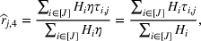
For each

$j\in [J]$

, define the effective lower bound

${\ell }_j^{\text{eff}}:=\max \{{\ell }_j,q_j^{\ast }\}$

. Theorem 2 characterizes the optimal capacity plan that solves the model (Basic), which is obtained based on Remark 3, Lemma EC.3 in the Supporting Information, Corollary 1, Theorem 1, and Proposition 4. Theorem 2 Characterization of the Optimal Capacity Plan

Either the model (Basic) is infeasible or there exists at most one lot

$k\in [J]$

such that

$C_k^{\ast }\in ({\ell }_k^{\text{eff}},u_k)$

and

$C_j^{\ast }\in \{{\ell }_j^{\text{eff}},u_j\}$

for all

$j\in [J]$

and

$j\ne k$

.

Theorem 2 implies that when the optimal capacity sizing model (Basic) is feasible, except for at most one lot k whose optimal capacity is strictly between the lower bound

${\ell }_j$

and upper bound

$u_j$

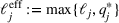
, the optimal capacity of each lot

$j\ne k$

is equal to one of the following three values:

${\ell }_j$

,

$u_j$

, and the optimal traffic flow

$q_j^{\ast }$

. The theorem also suggests that under an optimal capacity plan, one of the three constraints (14)–(16) is binding for each

$j\ne k$

in the model (Flow).

ALGORITHMS

In this section, we develop a one‐variable search algorithm to determine an optimal capacity plan. More specifically, first, we refine the feasible range of z in the model (Univar). Then, in Section 6.1, we propose an algorithm to determine the unique equilibrium flow pattern under any capacity plan, by which we can determine the refined feasible range of z. In Section 6.2, we present the one‐variable search algorithm.

Let

${\mathbf{q}}^L:=(q_j^L,j\in [J])$

denote the equilibrium flow pattern under the all‐lower‐bound capacity plan

${\mathbf{C}}^L:=({\ell }_1,{\ell }_2,\text{…},{\ell }_J)$

and

${\mathbf{q}}^H:=(q_j^H,j\in [J])$

denote the equilibrium flow pattern under the all‐upper‐bound capacity plan

${\mathbf{C}}^H:=(u_1,u_2,\text{…},u_J)$

. Proposition 5 provides a refined range of z that consists of all the feasible points of z to the model (Univar). Proposition 5

If

$z\in (0,1)$

is feasible to the model (Univar), then

$z\in [\parallel {\mathbf{q}}^L{\parallel }_1,\parallel {\mathbf{q}}^H{\parallel }_1]$

.

Proposition 5 indicates that the feasible region (0,1) of z can be replaced by

$[\parallel {\mathbf{q}}^L{\parallel }_1,\parallel {\mathbf{q}}^H{\parallel }_1]$

without excluding any feasible solutions in the model (Univar). The refined range will later be used in Algorithm 2 to speed up the solution procedure.

Solving the equilibrium flow pattern for a given capacity plan

We need to determine

${\mathbf{q}}^i$

under

${\mathbf{C}}^i$

for

$i\in \{L,H\}$

to obtain the refined range of z. To that end, in this section, we present in Algorithm 1 a solution procedure to solve the unique equilibrium flow pattern

$\mathbf{q}$

that satisfies

$\mathbf{q}=\mathbf{F}(\mathbf{q},\mathbf{C})$

under any given capacity plan

$\mathbf{C}\in {(0,\infty ]}^J$

.

ALGORITHM 1

Solving the equilibrium flows under a capacity plan

Input:J, $f_j$ in EC.17 for $j\in [J]$ , ${\delta }_1,{\delta }_2>0$ , $\text{ub}\leftarrow 1$ , $\text{lb}\leftarrow z^0$ , $z\leftarrow (\text{lb}+\text{ub})/2$ , and $\mathbf{C}$ .

Output: $\mathbf{q}$ such that $\mathbf{q}=\mathbf{F}(\mathbf{q},\mathbf{C})$ .

1:Find $q_j\in [0,1]$ such that $f_j(q_j)=\log (1-z)$ using Algorithm EC.1 for each $j\in [J]$ ;

2:Set $\mathrm{\Gamma }(z)\leftarrow {\sum }_{j=1}^J{q}_j-z$ ;

3:while $|\mathrm{\Gamma }(z)|>{\delta }_1$ and $\text{ub}-\text{lb}>{\delta }_2$ do

4:Set $\text{lb}\leftarrow z$ if $\mathrm{\Gamma }(z)>0$ ; set $\text{ub}\leftarrow z$ otherwise;

5:Set $z\leftarrow (\text{lb}+\text{ub})/2$ ;

6:Find $q_j\in [0,1]$ such that $f_j(q_j)=\log (1-z)$ using Algorithm EC.1 for each $j\in [J]$ ;

7:Set $\mathrm{\Gamma }(z)\leftarrow {\sum }_{j=1}^J{q}_j-z$ ;

8:end while

Algorithm 1 is developed based on Proposition EC.2 and the classical bisection search Algorithm EC.1 in the Supporting Information. The key idea is to treat the total traffic flow z under

$\mathbf{C}$

as a variable and show that the equilibrium z that satisfies the fixed‐point equation 

$\mathbf{q}=\mathbf{F}(\mathbf{q},\mathbf{C})$

is the unique root of a strictly decreasing and continuous function (cf. Proposition EC.2 in the Supporting Information). Then, the equilibrium z can be determined using the bisection search method (see Algorithm EC.1 in the Supporting Information) and the equilibrium flow pattern can be obtained using Proposition EC.2 in the Supporting Information. While Algorithm 1 will be used to determine

${\mathbf{q}}^L$

and

${\mathbf{q}}^H$

in Algorithm 2, it is useful in its own right in forecasting traffic flows under an MNL choice model.

A one‐variable search algorithm

In this section, we present in Algorithm 2 a solution procedure to determine an optimal capacity plan by solving the model (Univar) based on Corollary 1 and Theorem 1.

ALGORITHM 2

A one‐variable search method

Input:	φ, β, θ, J, $(b_j,j\in [J])$ , $({\ell }_j,j\in [J])$ , $(u_j,j\in [J])$ , ${\mathbf{C}}^L$ , ${\mathbf{C}}^H$ , $\mathrm{\Delta }z$ , $\mathcal{Z}\leftarrow ⌀$ .
Output:	${\mathbf{C}}^{\ast }$ .
Step 1.	Obtain ${\mathbf{q}}^i$ by solving ${\mathbf{q}}^i=\mathbf{F}({\mathbf{q}}^i,{\mathbf{C}}^i)$ for $i\in \{L,H\}$ using Algorithm 1. Set $z\leftarrow \parallel {\mathbf{q}}^L{\parallel }_1$ .
Step 2.	If $z>\parallel {\mathbf{q}}^H{\parallel }_1$ , go to Step 6; execute the following otherwise. Set $\stackrel{\sim }{\mathcal{Q}}\leftarrow ⌀$ , $k\leftarrow 1$ , and $n\leftarrow 1$ . If there exists $j\in [J]$ such that $\log (1-z)+b_j+\phi >\beta +\phi \min \{1,1/{\ell }_j\}$ , then set $z\to z+\mathrm{\Delta }z$ and go to Step 2; go to Step 3 otherwise.
Step 3.	For each $j\in [J]$ , solve $x_k^{\ast }\in (0,1]$ such that ${\zeta }_{j,k}(x_k^{\ast },z)=0$ for $k\in \{1,2\}$ using Algorithm EC.1 and set $q_j^L(z)\leftarrow \max \{x_1^{\ast },x_2^{\ast }\}$ .
Step 4.	For each $j\in [J]$ , if $\log (1-z)+b_j+\phi >\beta +\phi /u_j$ , set $q_j^H(z)\leftarrow 1$ ; Otherwise, solve $x_3^{\ast }\in (0,1]$ such that ${\zeta }_{j,3}(x_3^{\ast },z)=0$ using Algorithm EC.1, set $q_j^H(z)\leftarrow x_3^{\ast }$ if $x_3^{\ast }\le u_j$ , and set $z\to z+\mathrm{\Delta }z$ and go to Step 2 if $x_3^{\ast }>u_j$ .
Step 5.	Set $\mathbf{q}=(q_j,j\in [J])\leftarrow$ The n‐th element in ${\widehat{\mathcal{Q}}}^k(z)$ as defined in (22). If $q_k\in [q_k^L(z),q_k^H(z)]$ , set $\stackrel{\sim }{\mathcal{Q}}\leftarrow \stackrel{\sim }{\mathcal{Q}}\cup \{\mathbf{q}\}$ . Then, execute the following:
	(a) If $n<|{\widehat{\mathcal{Q}}}^k(z)|$ , set $n\leftarrow n+1$ and go to Step 5; (b) If $k<J$ and $n=|{\widehat{\mathcal{Q}}}^k(z)|$ , set $k\leftarrow k+1$ , $n\leftarrow 1$ , and go to Step 5; (c) If $k=J$ and $n=|{\widehat{\mathcal{Q}}}^k(z)|$ , find ${\mathbf{q}}^{\ast }(z):=(q_j^{\ast }(z),j\in [J])\in arg{\max }_{\mathbf{q}\in \stackrel{\sim }{\mathcal{Q}}}{\sum }_{j=1}^J{q}_j\log (q_j)$ , set $\widehat{h}(z)={\sum }_{j=1}^J{q}_j^{\ast }(z)\log (q_j^{\ast }(z))$ , calculate $\pi (z)=\widehat{h}(z)-z\log (1-z)$ , set $\mathcal{Z}\leftarrow \mathcal{Z}\cup \{z\}$ , set $z\to z+\mathrm{\Delta }z$ , and go to Step 2;
Step 6.	Find $z^{\ast }\in {\arg \max }_{z\in \mathcal{Z}}\pi (z)$ . Set ${\mathbf{C}}^{\ast }\leftarrow \mathit{\xi }({\mathbf{q}}^{\ast }(z^{\ast }))$ , where ξ is defined in (13).

Discretizing z

In Algorithm 2, we discretize the range

$[\parallel {\mathbf{q}}^L{\parallel }_1,\parallel {\mathbf{q}}^H{\parallel }_1]$

with a step size of

$\mathrm{\Delta }z>0$

. For each discretized value of z, we will calculate the objective value

$\pi (z)$

in the model (Univar). Then, an optimal solution

$z^{\ast }$

can be obtained by comparing

$\pi (z)$

at all discretized values (cf. Step 6).

Generating candidate optimal solutions to the model (Sub)

For each discretized z, we need to solve the model (Sub) to obtain

$\widehat{h}(z)$

, by which we can compute

$\pi (z)=\widehat{h}(z)-z\log (1-z)$

.

We can determine an optimal solution

${\mathbf{q}}^{\ast }(z)$

to the model (Sub) (if feasible) using Theorem 1, which suggests that there exists at most one lot k such that

$q_k^{\ast }(z)$

is between

$q_k^L(z)$

and

$q_k^H(z)$

and

$q_j^{\ast }(z)$

is equal to either

$q_j^L(z)$

or

$q_j^H(z)$

for any lot

$j\ne k$

.

For each such k, we can generate a candidate

${\mathbf{q}}^{\ast }(z)$

as follows. Assign

$q_j^L(z)$

or

$q_j^H(z)$

to

$q_j^{\ast }(z)$

for all

$j\ne k$

and calculate

$q_k^{\ast }(z)=z-{\sum }_{j\ne k}{q}_j^{\ast }(z)$

. If

$q_k^{\ast }(z)\in [q_k^L(z),q_k^H(z)]$

, the

${\mathbf{q}}^{\ast }(z)$

so generated is a valid candidate optimal solution; it is nonvalid and will be dropped otherwise. To facilitate the exposition of the generation of candidate

${\mathbf{q}}^{\ast }(z)$

in Algorithm 2, let

${\widehat{\mathcal{Q}}}^k(z)$

denote the set of (valid and nonvalid) candidate

${\mathbf{q}}^{\ast }(z)$

generated for any

$k\in [J]$

, which is represented by

22

Then, as in Step 5, we can obtain

$\widehat{h}(z)$

by comparing the objective values in the model (Sub) at all valid candidate

${\mathbf{q}}^{\ast }(z)$

in

${\widehat{\mathcal{Q}}}^k(z)$

for all

$k\in [J]$

. Note

$|{\widehat{\mathcal{Q}}}^k(z)|\le 2^{J-1}$

.

More discussions on

${\widehat{\mathcal{Q}}}^k(z)$

For each discretized z, we find a flow pattern

${\mathbf{q}}^{\ast }(z)$

that satisfies (21) for all

$j\ne k$

and is thus a candidate optimal solution to the model (Sub). It further requires that the total traffic flow

$\parallel {\mathbf{q}}^{\ast }{(z)\parallel }_1$

is equal to z. The set

${\widehat{\mathcal{Q}}}^k(z)$

consists of all such

${\mathbf{q}}^{\ast }(z)$

s.

Feasibility check and expedition

Algorithm 2 involves procedures skipping infeasible values of z in Step 2 and Step 4, by which the solution procedure is expedited. The feasibility of each discretized z is checked using the conditions provided in Corollary 1. More specifically, if

${\mathcal{Q}}_j(z)=[q_j^L(z),q_j^H(z)]=⌀$

for some j at z, then such z is infeasible. Note that

$q_j^L(z)$

and

$q_j^H(z)$

can be obtained as in Corollary 1 using Algorithm EC.1 in the Supporting Information.

NUMERICAL EXPERIMENTS

In this section, we provide numerical results to gain insights into the optimal capacity design for park‐and‐ride lots in a satellite city and to investigate the value of modeling the congestion and parking effects in optimal sizing of park‐and‐ride lots. In Section 7.1, we describe the data related to the park‐and‐ride lots in Bellevue of Washington State (WA). In Section 7.2, we apply our developed models and algorithms to solve the optimal capacities of Bellevue's park‐and‐ride lots. Section 7.3 provides sensitivity analysis. In Section 7.4, we evaluate the performance of the optimal capacity plan under different choice behavior of commuters.

The model (Univar) is solved using Algorithm 2 with

$\mathrm{\Delta }z={10}^{-7}$

and the numerical results are obtained using Matlab R2022a on a desktop computer with Intel i7 CPU@3.20 GHz and 16 GB RAM.

Bellevue's park‐and‐ride lots and data

In this section, we study the park‐and‐ride lots in the city of Bellevue in Washington State (WA), which is a satellite city of Seattle.

According to King County Metro (2022a), there are

$J=7$

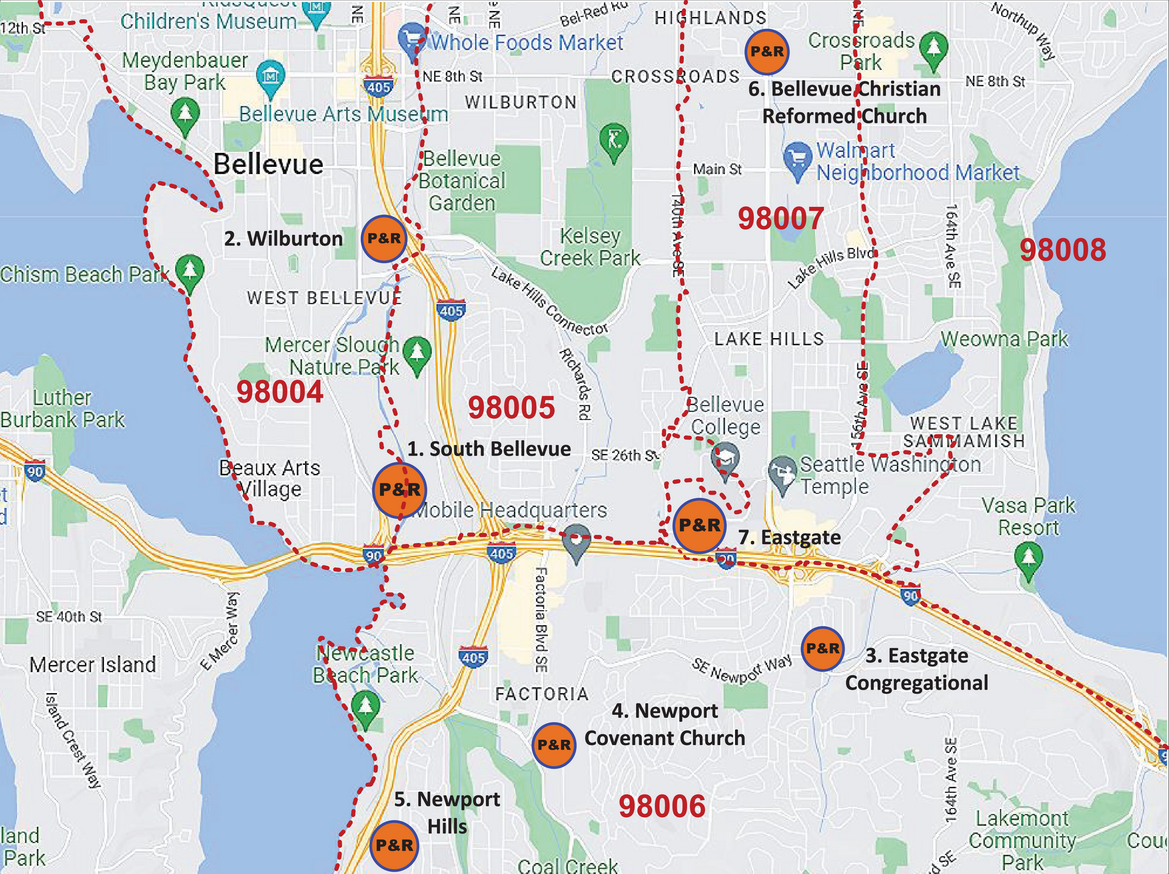
park‐and‐ride lots accessible to commuters in Bellevue. Figure 2 shows the names and locations of the lots on the map of Bellevue. Table EC.1 in the Supporting Information shows their addresses and current capacities.

FIGURE 2

The names and locations of the park‐and‐ride lots in Bellevue, WA (King County Metro, 2022a).

We will (re)design the capacities of these lots using our developed models and algorithms. The objective of this section is twofold: (i) to demonstrate that our models and algorithms can be applied to real‐world cases, where the DOT needs to design a set of new park‐and‐ride lots or redesign existing lots to accommodate the growing demand for parking electric vehicles, and (ii) to obtain insights into the optimal capacity design of park‐and‐ride lots in a satellite city such as Bellevue.

Determining catchment areas

We geographically partition Bellevue into seven catchment areas such that each catchment area contains a single park‐and‐ride lot, the entire Bellevue is the union of all the catchment areas, and the catchment areas of any two different lots do not overlap. The catchment area of any lot is an area where commuters would choose to visit that lot (rather than others) if they base their decisions solely on congestion‐free travel time. Let

$H_j\in {\mathbb{R}}_{+}$

denote the number of households in the catchment area of any lot

$j\in [J]$

, which is provided in Table EC.2 in the Supporting Information. The catchment areas and

$H_j$

s are determined in Section EC.5.2 in the Supporting Information.

Table EC.3 in the Supporting Information shows bidirectional time distances between different pairs

$(i,j)$

of lots in Bellevue, where

$i,j\in [J]$

, which are collected around 3 a.m. on October 8, 2022 (Saturday), using Google Map (2022). Since congestion seldom occurs around 3 a.m. on a Saturday morning, these data can be used to approximate the congestion‐free travel time from the catchment area of a lot

$i\in [J]$

to that of a lot

$j\in [J]$

, which is denoted by

${\tau }_{i,j}\in {\mathbb{R}}_{+}$

.

Next, we estimate the values of attributes such as the economic value, number of bus routes, bus frequency, and congestion‐free access time, which will be used to estimate the intrinsic utilities of Bellevue's park‐and‐ridelots.

Economic value

Let

${\widehat{r}}_{j,1}\in {\mathbb{R}}_{+}$

denote the economic value of any lot

$j\in [J]$

, which is represented by the median house/condo value for j as shown in Table EC.2 in the Supporting Information. The median house/condo value for each

$j\in [J]$

is the median value of the houses/condominiums in the area with the same zip code as j, which reflects the economic value of js location and is obtained from City‐Data (2016).

The number of bus routes

There is a bus stop next to each lot, through which commuters access transit services. Let

${\widehat{r}}_{j,2}\in {\mathbb{R}}_{+}$

denote the number of bus routes traversing (the bus stop next to) lot j, which is provided in Table EC.2 in the Supporting Information and obtained from King County Metro (2022a).

Bus frequency

Let

${\widehat{r}}_{j,3}\in {\mathbb{R}}_{+}$

denote the bus frequency that measures the frequency of bus arrivals at lot j, which is estimated as follows. For each bus route passing by j, we calculate the average interarrival time (in minutes) of the buses arriving at j between 7 a.m. and 9 a.m. on workdays using King County Metro (2022b) and Sound Transit (2022). Next, the average bus headway for j as shown in Table EC.2 in the Supporting Information is calculated as the mean of the average interarrival times for all the bus routes passing along j. Then,

${\widehat{r}}_{j,3}$

can be computed as the reciprocal of the average bus headway for j.

Congestion‐free access time

Let

${\widehat{r}}_{j,4}\in {\mathbb{R}}_{+}$

denote the congestion‐free access time to lot j as shown in Table EC.2 in the Supporting Information, which is the average travel time to j per trip (or vehicle) under no congestion. Let η denote the average number of park‐and‐ride trips per household on a workday morning. Hence,

$H_j\eta$

approximates the number of commuters' trips generated from the catchment area of j. Then,

${\widehat{r}}_{j,4}$

can be estimated by

$$\begin{array}{c}\hfill {\widehat{r}}_{j,4}=\frac{{\sum }_{i\in [J]}{H}_i\eta {\tau }_{i,j}}{{\sum }_{i\in [J]}{H}_i\eta }=\frac{{\sum }_{i\in [J]}{H}_i{\tau }_{i,j}}{{\sum }_{i\in [J]}{H}_i},\end{array}$$

where we assume that for the commuters generated from the catchment area of any lot, the congestion‐free travel time to that lot is zero.

Scaling

We will conduct sensitivity analysis in Section 7.3 to investigate and compare the impacts of the sensitivities of commuters to different attributes on optimal capacity sizing. Since the data in Table EC.2 in the Supporting Information are of different scales, it often requires scaling the data to facilitate the comparison (and make optimization used to estimate the choice model well conditioned; Lantz, 2013). To that end, we choose the South Bellevue (i.e.,

$j=1$

) as the reference lot. Then, we obtain

$r_{j,k}:={\widehat{r}}_{j,k}/{\widehat{r}}_{1,k}$

as the normalized attribute value for all

$j\in [J]$

and

$k\in \{1,2,3,4\}$

, which is provided in Table EC.4 in the Supporting Information.

Then, for each

$j\in [J]$

, the intrinsic utility

$b_j$

can be estimated by,

$$b_j={\alpha }_1{r}_{j,1}+{\alpha }_2{r}_{j,2}+{\alpha }_3{r}_{j,3}-{\alpha }_4{r}_{j,4},$$

23

where

${\alpha }_k\in {\mathbb{R}}_{+}$

is the sensitivity parameter for

$k\in \{1,2,3,4\}$

.

Optimal capacities and flows under different lower and upper bound capacities

In this section, we solve the optimal capacity sizing problem for Bellevue's park‐and‐ride lots.

We set

${\alpha }_k=2.5$

for all

$k\in \{1,2,3,4\}$

,

$\beta =2.5$

,

$\theta =0.5$

, and

$\phi =2.5$

throughout this section, where the parameters are arbitrarily chosen and we will explore the influence of the variations in these parameters on optimal solutions in Section 7.3.

We choose South Bellevue (i.e.,

$j=1$

) as the reference lot. First, we select values of ℓ₁ and u ₁. Then, for any lot

$j\in \{2,3,\text{…},7\}$

,

${\ell }_j$

(

$u_j$

) is computed as ℓ₁ (u ₁) multiplied by the ratio of the current capacity of lot j (cf. Table EC.1 in the Supporting Information) to that of South Bellevue, by which the relative sizes of the lower and upper bounds of all the lots are consistent with the relative sizes of their current capacities.

We obtain numerical results for a variety of cases specified by different values of ℓ₁ and u ₁ (as well as different lower and upper bounds for

$j\in \{2,3,\text{…},7\}$

determined as previously mentioned). Define

${\rho }_j^{\ast }:=q_j^{\ast }/C_j^{\ast }$

as the optimal utilization at lot

$j\in [J]$

. Tables 2 and 3 show the intrinsic utilities, optimal capacities, traffic flows, and utilizations under different cases of ℓ₁ and u ₁. Table EC.5 in the Supporting Information shows the same content as Tables 2 and 3 except that different ℓ₁ and u ₁ are considered to provide results under a broader range of lower and upper bounds.

TABLE 2

The optimal capacities, traffic flows, and utilizations under

${\ell }_1\in \{0.05,0.25,0.5,0.7\}$

and

$u_1\in \{0.75,0.85\}$

.

		${\ell }_1=0.05$ , $u_1=0.75$					${\ell }_1=0.05$ , $u_1=0.85$
j	$b_j$	${\ell }_j$	$u_j$	$C_j^{\ast }$	$q_j^{\ast }$	${\rho }_j^{\ast }$	${\ell }_j$	$u_j$	$C_j^{\ast }$	$q_j^{\ast }$	${\rho }_j^{\ast }$
1	5.0000	0.0500	0.7500	0.7500	0.2612	34.82%	0.0500	0.8500	0.8500	0.2538	29.85%
2	2.4119	0.0062	0.0930	0.0930	0.0376	40.48%	0.0062	0.1054	0.1054	0.0367	34.85%
3	1.6794	0.0007	0.0100	0.0055	0.0055	100.00%	0.0007	0.0113	0.0048	0.0048	100.00%
4	2.5824	0.0025	0.0375	0.0375	0.0251	67.02%	0.0025	0.0425	0.0425	0.0254	59.70%
5	1.3456	0.0092	0.1375	0.1369	0.0248	18.13%	0.0092	0.1558	0.1558	0.0231	14.80%
6	‐0.4637	0.0007	0.0100	0.0007	0.0007	100.00%	0.0007	0.0113	0.0007	0.0007	97.72%
7	7.7539	0.0538	0.8070	0.8070	0.6437	79.77%	0.0538	0.9146	0.9146	0.6546	71.57%

		${\ell }_1=0.25$ , $u_1=0.75$					${\ell }_1=0.25$ , $u_1=0.85$
j	$b_j$	${\ell }_j$	$u_j$	$C_j^{\ast }$	$q_j^{\ast }$	${\rho }_j^{\ast }$	${\ell }_j$	$u_j$	$C_j^{\ast }$	$q_j^{\ast }$	${\rho }_j^{\ast }$
1	5.0000	0.2500	0.7500	0.7500	0.2607	34.76%	0.2500	0.8500	0.8500	0.2534	29.81%
2	2.4119	0.0310	0.0930	0.0930	0.0376	40.40%	0.0310	0.1054	0.1054	0.0367	34.79%
3	1.6794	0.0033	0.0100	0.0056	0.0056	99.18%	0.0033	0.0113	0.0047	0.0047	100.00%
4	2.5824	0.0125	0.0375	0.0375	0.0251	66.91%	0.0125	0.0425	0.0425	0.0253	59.63%
5	1.3456	0.0458	0.1375	0.1375	0.0248	18.03%	0.0458	0.1558	0.1552	0.0230	14.81%
6	‐0.4637	0.0033	0.0100	0.0033	0.0020	58.61%	0.0033	0.0113	0.0033	0.0018	54.70%
7	7.7539	0.2690	0.8070	0.8070	0.6430	79.68%	0.2690	0.9146	0.9146	0.6540	71.51%

		${\ell }_1=0.5$ , $u_1=0.75$					${\ell }_1=0.5$ , $u_1=0.85$
j	$b_j$	${\ell }_j$	$u_j$	$C_j^{\ast }$	$q_j^{\ast }$	${\rho }_j^{\ast }$	${\ell }_j$	$u_j$	$C_j^{\ast }$	$q_j^{\ast }$	${\rho }_j^{\ast }$
1	5.0000	0.5000	0.7500	0.7500	0.2602	34.69%	0.5000	0.8500	0.8500	0.2527	29.73%
2	2.4119	0.0620	0.0930	0.0930	0.0375	40.30%	0.0620	0.1054	0.1054	0.0366	34.69%
3	1.6794	0.0067	0.0100	0.0069	0.0064	93.06%	0.0067	0.0113	0.0067	0.0060	89.17%
4	2.5824	0.0250	0.0375	0.0375	0.0250	66.79%	0.0250	0.0425	0.0425	0.0253	59.48%
5	1.3456	0.0917	0.1375	0.1375	0.0247	17.97%	0.0917	0.1558	0.1558	0.0229	14.70%
6	‐0.4637	0.0067	0.0100	0.0067	0.0028	42.56%	0.0067	0.0113	0.0067	0.0026	39.20%
7	7.7539	0.5380	0.8070	0.8070	0.6422	79.57%	0.5380	0.9146	0.9146	0.6529	71.39%

		${\ell }_1=0.7$ , $u_1=0.75$					${\ell }_1=0.7$ , $u_1=0.85$
j	$b_j$	${\ell }_j$	$u_j$	$C_j^{\ast }$	$q_j^{\ast }$	${\rho }_j^{\ast }$	${\ell }_j$	$u_j$	$C_j^{\ast }$	$q_j^{\ast }$	${\rho }_j^{\ast }$
1	5.0000	0.7000	0.7500	0.7500	0.2595	34.60%	0.7000	0.8500	0.8500	0.2521	29.66%
2	2.4119	0.0868	0.0930	0.0930	0.0374	40.19%	0.0868	0.1054	0.1054	0.0365	34.59%
3	1.6794	0.0093	0.0100	0.0095	0.0079	83.50%	0.0093	0.0113	0.0093	0.0074	79.47%
4	2.5824	0.0350	0.0375	0.0375	0.0250	66.64%	0.0350	0.0425	0.0425	0.0252	59.36%
5	1.3456	0.1283	0.1375	0.1375	0.0246	17.90%	0.1283	0.1558	0.1554	0.0228	14.68%
6	‐0.4637	0.0093	0.0100	0.0093	0.0033	35.57%	0.0093	0.0113	0.0093	0.0030	32.55%
7	7.7539	0.7532	0.8070	0.8070	0.6411	79.44%	0.7532	0.9146	0.9146	0.6519	71.28%

TABLE 3

The optimal capacities, traffic flows, and utilizations under

${\ell }_1\in \{0.05,0.25,0.5,0.7\}$

and

$u_1\in \{0.95,1\}$

.

		${\ell }_1=0.05$ , $u_1=0.95$					${\ell }_1=0.05$ , $u_1=1$
j	$b_j$	${\ell }_j$	$u_j$	$C_j^{\ast }$	$q_j^{\ast }$	${\rho }_j^{\ast }$	${\ell }_j$	$u_j$	$C_j^{\ast }$	$q_j^{\ast }$	${\rho }_j^{\ast }$
1	5.0000	0.0500	0.9500	0.9500	0.2525	26.58%	0.0500	1.0000	1.0000	0.2493	24.93%
2	2.4119	0.0062	0.1178	0.1178	0.0368	31.20%	0.0062	0.1240	0.1240	0.0363	29.30%
3	1.6794	0.0007	0.0127	0.0043	0.0043	100.00%	0.0007	0.0133	0.0041	0.0041	100.00%
4	2.5824	0.0025	0.0475	0.0473	0.0260	54.92%	0.0025	0.0500	0.0500	0.0261	52.23%
5	1.3456	0.0092	0.1742	0.0092	0.0064	69.71%	0.0092	0.1833	0.0093	0.0063	67.78%
6	‐0.4637	0.0007	0.0127	0.0007	0.0006	95.19%	0.0007	0.0133	0.0007	0.0006	93.48%
7	7.7539	0.0538	1.0222	1.0222	0.6725	65.79%	0.0538	1.0760	1.0760	0.6763	62.86%

		${\ell }_1=0.25$ , $u_1=0.95$					${\ell }_1=0.25$ , $u_1=1$
j	$b_j$	${\ell }_j$	$u_j$	$C_j^{\ast }$	$q_j^{\ast }$	${\rho }_j^{\ast }$	${\ell }_j$	$u_j$	$C_j^{\ast }$	$q_j^{\ast }$	${\rho }_j^{\ast }$
1	5.0000	0.2500	0.9500	0.9500	0.2470	26.00%	0.2500	1.0000	1.0000	0.2441	24.41%
2	2.4119	0.0310	0.1178	0.1178	0.0359	30.44%	0.0310	0.1240	0.1240	0.0355	28.61%
3	1.6794	0.0033	0.0127	0.0041	0.0041	100.00%	0.0033	0.0133	0.0039	0.0039	100.00%
4	2.5824	0.0125	0.0475	0.0475	0.0255	53.77%	0.0125	0.0500	0.0500	0.0256	51.25%
5	1.3456	0.0458	0.1742	0.1712	0.0215	12.55%	0.0458	0.1833	0.1822	0.0209	11.48%
6	‐0.4637	0.0033	0.0127	0.0033	0.0017	51.65%	0.0033	0.0133	0.0033	0.0017	50.35%
7	7.7539	0.2690	1.0222	1.0222	0.6633	64.89%	0.2690	1.0760	1.0760	0.6675	62.03%

		${\ell }_1=0.5$ , $u_1=0.95$					${\ell }_1=0.5$ , $u_1=1$
j	$b_j$	${\ell }_j$	$u_j$	$C_j^{\ast }$	$q_j^{\ast }$	${\rho }_j^{\ast }$	${\ell }_j$	$u_j$	$C_j^{\ast }$	$q_j^{\ast }$	${\rho }_j^{\ast }$
1	5.0000	0.5000	0.9500	0.9500	0.2463	25.93%	0.5000	1.0000	1.0000	0.2433	24.33%
2	2.4119	0.0620	0.1178	0.1178	0.0357	30.34%	0.0620	0.1240	0.1240	0.0353	28.51%
3	1.6794	0.0067	0.0127	0.0067	0.0057	85.72%	0.0067	0.0133	0.0067	0.0056	84.15%
4	2.5824	0.0250	0.0475	0.0475	0.0255	53.64%	0.0250	0.0500	0.0500	0.0256	51.11%
5	1.3456	0.0917	0.1742	0.1652	0.0212	12.86%	0.0917	0.1833	0.1787	0.0207	11.60%
6	‐0.4637	0.0067	0.0127	0.0067	0.0024	36.62%	0.0067	0.0133	0.0067	0.0024	35.53%
7	7.7539	0.5380	1.0222	1.0222	0.6622	64.78%	0.5380	1.0760	1.0760	0.6662	61.91%

		${\ell }_1=0.7$ , $u_1=0.95$					${\ell }_1=0.7$ , $u_1=1$
j	$b_j$	${\ell }_j$	$u_j$	$C_j^{\ast }$	$q_j^{\ast }$	${\rho }_j^{\ast }$	${\ell }_j$	$u_j$	$C_j^{\ast }$	$q_j^{\ast }$	${\rho }_j^{\ast }$
1	5.0000	0.7000	0.9500	0.9500	0.2457	25.86%	0.7000	1.0000	1.0000	0.2428	24.28%
2	2.4119	0.0868	0.1178	0.1178	0.0356	30.26%	0.0868	0.1240	0.1240	0.0353	28.44%
3	1.6794	0.0093	0.0127	0.0093	0.0071	75.99%	0.0093	0.0133	0.0093	0.0070	74.52%
4	2.5824	0.0350	0.0475	0.0475	0.0254	53.52%	0.0350	0.0500	0.0500	0.0255	51.02%
5	1.3456	0.1283	0.1742	0.1675	0.0212	12.67%	0.1283	0.1833	0.1726	0.0205	11.89%
6	‐0.4637	0.0093	0.0127	0.0093	0.0028	30.24%	0.0093	0.0133	0.0093	0.0027	29.28%
7	7.7539	0.7532	1.0222	1.0222	0.6612	64.68%	0.7532	1.0760	1.0760	0.6653	61.83%

We observe the following from Tables 2, 3, and EC.5 in the Supporting Information.

• (1)

A lot with a high intrinsic utility tends to attain the optimal capacity on the upper bound. If a lot has a low/moderate‐sized intrinsic utility and a small lower bound, its optimal capacity tends to be equal to the optimal traffic flow through the lot, yielding high utilization at the lot. However, a lot with a low/moderate‐sized intrinsic utility and a lower bound that is not small tends to attain the optimal capacity on the lower bound. For example, Lot 6 attains its optimal capacity on the lower bound when ℓ₁ exceeds a threshold value (e.g., when

${\ell }_1>0.05$

). Since

$b_6=-0.4637<0$

, Lot 6 is potentially less attractive to commuters than other lots and the no‐park‐and‐ride alternative. Therefore, it tends to be optimal to set the optimal capacity

$C_6^{\ast }={\ell }_6$

to accommodate the limited demand it attracts, provided that ℓ₆ is not smaller than the demand (which happens when ℓ₁ is not small). However, when ℓ₆ is smaller than the demand (which happens when ℓ₁ is small, e.g., when

${\ell }_1=0.05$

), it is optimal to set

$C_6^{\ast }=q_6^{\ast }$

to accommodate the demand, resulting in the utilization of 100% of the lot.

(2)

In general, a lot with a large (small) intrinsic utility tends to attract a high (low) traffic flow. However, this is not always true: A lot with a high intrinsic utility and high parking utilization may attract fewer commuters than that with a low intrinsic utility and low utilization. For example, if commuters base their decisions only on intrinsic utilities,

$q_2^{\ast }\le q_4^{\ast }$

holds under all cases since

$b_2<b_4$

. When commuters are additionally information aware, we have

$q_2^{\ast }=0.0376>q_4^{\ast }=0.0251$

under the case of

${\ell }_1=0.25$

and

$u_1=0.75$

, since Lot 2 has higher parking availability than Lot 4. Thus, under an optimal capacity plan, it tends to reallocate information‐aware commuters from high‐utilization lots to low‐utilization lots. This finding highlights the impact of parking information on capacity sizing with information‐aware commuters.

(3)

The parking availability at a high‐utilization lot may not be improved by allowing for a smaller lower or a larger upper bound for the lot. For example, although Lot 3 has high utilization, the utilization may not drop and commuters may not be better off if the DOT allows for a different lower or upper bound for the lot. When

${\ell }_1=0.5,u_1=0.75$

,

$C_3^{\ast }$

is strictly between ℓ₃ and u ₃, indicating nonbinding lower and upper bound constraints. Hence, the utilization will not drop even when ℓ₃ decreases or u ₃ increases.

(4)

It is possibly both inevitable and beneficial to deploy lots around the peripheral area of a satellite city, and a peripheral lot may gain full or nearly full utilization. Examples include Lots 3 and 6 in Bellevue. On the one hand, practically, these lots are needed to provide nearby households with points of access to public transit, as the transit center is usually distant from the peripheral area (e.g., Bellevue Transit Center is located in the downtown). Analytically, even though a peripheral lot is initially used by very few commuters, it will gain more visits when the system reaches equilibrium due to the effects of congestion and parking information. Meanwhile, it seems reasonable not to set large upper bounds for the lots in the peripheral area. After all, a peripheral lot attracts a limited number of commuters due to its long access time and limited bus services near the lot, the optimal capacity tends to be equal to the effective lower bound.

(5)

It seems desirable to have a large‐sized lot close to the downtown area as long as the budget and space allow. However, the lot may not gain a good utilization rate, possibly due to the long bus waiting time caused by congestion. An example is Lot 2, which is close to downtown Bellevue. As Table EC.2 in the Supporting Information shows, Lot 2 has the longest average bus headway, that is, the average interarrival time between two consecutive buses, which jeopardizes its attractiveness to morning commuters who are eager to arrive at their office as early as possible, and thus, results in a low utilization rate.

Optimal capacities with unused lots

We have thus far considered that all the seven candidate lots are opened with positive lower bounds on their capacities. Our model and algorithms are also applicable when the DOT is allowed to use only a subset of the lots. Let

$\overline{J}\in \{1,2,\text{…},7\}$

denote the number of used lots. Figure EC.1 in the Supporting Information shows the optimal total social welfare as a function of

$\overline{J}$

under different upper bounds (indicated by different u ₁) but no lower bounds. We observe the following: (i) Opening only one lot may be unable to accommodate the need of all commuters, particularly when the upper bound is not large enough, for example, when

$u_1\in \{0.75,0.85\}$

; (ii) Opting to open only a portion of the lots may lead to a higher overall social welfare compared to utilizing all available lots. For example, the maximum total social welfare when

$\overline{J}=3$

is greater than that when

$\overline{J}=7$

.

Sensitivity analysis

In this section, we investigate how the changes in the sensitivity parameters

${\alpha }_k$

for

$k\in \{1,2,3,4\}$

, β, and φ affect optimal capacities.

We choose

${\ell }_1=0.25$

and

$u_1=0.75$

. Then, the lower and upper bounds for all lots are shown in Table 2. Figures EC.2–EC.7 in the Supporting Information show the optimal capacity and traffic flow of each Bellevue's park‐and‐ride lot as functions of α₁, α₂, α₃, α₄, β, and φ, respectively, and Figure 3 shows the optimal utilization of each lot as a function of φ. In each figure, the optimal capacities, traffic flows, or utilizations are obtained under different values of a particular sensitivity parameter, while the values of all other sensitivity parameters are fixed and as specified in Section 7.2.

FIGURE 3

The optimal utilization

${\rho }_j^{\ast }$

as a function of φ for all

$j\in \{1,2,\text{…},7\}$

.

We make the following observations from Figures EC.2–EC.7 in the Supporting Information and 3.

• (1)

As commuters become more sensitive to a particular attribute, such as economic value, the number of bus routes, bus frequency, or congestion‐free access time, the optimal traffic flows through the lots with large values of the attribute tends to be increasing, while those through the lots with small values of the attribute appear to be nonincreasing. For example, as α₂ increases, the optimal traffic flow through Lot 7 is increasing, while that through any other lot is decreasing. With a larger α₂, commuters are more sensitive to the number of bus routes passing by a lot. Since there are 14 bus routes serving Lot 7, which exceeds the number of bus routes passing through all other lots by at least nine, Lot 7 is likely to attract commuters from other lots as α₂ increases.

(2)

As commuters become more sensitive to congestion, it tends to reallocate commuters from lots with high traffic flows to those with low traffic flows under the optimal capacity plan. For example, Lot 7 has the largest traffic flow among all lots when commuters are congestion insensitive, that is, when

$\beta =0$

. As β increases, the optimal traffic flow through Lot 7 decreases, while that through any other lot increases.

(3)

As commuters become more sensitive to parking information, the utilization of a lot with high initial utilization tends to be nonincreasing, while that of a lot with low initial utilization tends to be nondecreasing with possible jumps to lower values. For example, the former result applies to Lots 3, 4, and 7, while the latter result applies to Lots 1, 2, 5, and 6.

(4)

For any lot, the optimal capacity seems to be nondecreasing in the optimal traffic flow. This is likely due to the capacity constraint

$q_j\le C_j$

for all

$j\in [J]$

in the model (Basic).

The performance of the optimal capacity plan under real‐time parking information

In this section, we use simulation to evaluate the performance of the optimal capacity plan for Bellevue's park‐and‐ride lots when commuters are provided with (and sensitive to) real‐time parking information. To that end, we first introduce three capacity plans to be compared as follows:

${\mathbf{C}}^{\ast }$

:

The DOT considers that commuters are information‐, congestion‐, and intrinsic‐utility aware, solves the model (Basic), and obtains the optimal capacity plan

${\mathbf{C}}^{\ast }$

.

${\mathbf{C}}^1$

:

(The congestion effect is ignored) The DOT considers that commuters are information‐ and intrinsic‐utility aware but congestion unaware, which is equivalent to treating β as zero, solves the model (Basic) (with

$\beta =0$

), and obtains the optimal solution as

${\mathbf{C}}^1$

.

${\mathbf{C}}^2$

:

(The parking effect is ignored) The DOT considers that commuters are congestion‐ and intrinsic‐utility aware but information unaware, which is equivalent to presuming

$\phi =0$

. Then, the DOT solves the fixed‐point equation (5) (with

$\phi =0$

) using Algorithm 1 and obtains the equilibrium flow pattern

$\stackrel{\sim }{\mathbf{q}}=({\stackrel{\sim }{q}}_1,{\stackrel{\sim }{q}}_2,\text{…},{\stackrel{\sim }{q}}_J)$

. The DOT sets

${\stackrel{\sim }{C}}_j:=\min \{\max \{{\ell }_j,{\stackrel{\sim }{q}}_j\},u_j\}$

for all

$j\in [J]$

and obtains the capacity plan

${\mathbf{C}}^2:=({\stackrel{\sim }{C}}_j,j\in [J])$

.

Then, in Section EC.5.1 in the Supporting Information, we define nine choice scenarios, describe the departure process of commuters, and build commuter choice models under real‐time parking information and different choice scenarios. To evaluate the performance of the optimal capacity plan

${\mathbf{C}}^{\ast }$

, we will compare the expected total social welfare generated by

${\mathbf{C}}^{\ast }$

,

${\mathbf{C}}^1$

, and

${\mathbf{C}}^2$

under the nine choice scenarios.

Next, we generate the departures and choices of commuters using simulation, and then calculate the expected total social welfare (i.e.,

${\mathrm{\Pi }}^m(\mathbf{C})$

in (EC.21)) using sample average approximations.

We set

$T=7,200$

s to account for commuters departing within 7–9 a.m. on Mondays and

$\kappa =1$

. Hence,

$Q=\lfloor 7200\kappa \rfloor$

. The values of

$r_{j,k}$

s are as in Table EC.4 in the Supporting Information and those of

${\alpha }_k$

for

$k\in \{1,2,3,4\}$

, θ, β, and φ are as specified in Section 7.2. Similar to Section 7.2, the comparison results are obtained under different lower and upper bounds.

For each choice scenario

$m\in \{1,2,\text{…},9\}$

and capacity plan

$\mathbf{C}\in \{{\mathbf{C}}^{\ast },{\mathbf{C}}^1,{\mathbf{C}}^2\}$

, let

${\overline{\mathrm{\Pi }}}^m(\mathbf{C})$

denote the sample average approximation of

${\mathrm{\Pi }}^m(\mathbf{C})$

computed using 1,000 sample paths of the joint departure and choice processes of commuters. Define the relative gap

$$\begin{array}{c}\hfill {\text{Gap}}_i^m:=\frac{{\overline{\mathrm{\Pi }}}^m({\mathbf{C}}^{\ast })-{\overline{\mathrm{\Pi }}}^m({\mathbf{C}}^i)}{|{\overline{\mathrm{\Pi }}}^m({\mathbf{C}}^{\ast })|}\times 100,\end{array}$$

for each m and the total relative gap TG

${}_i:={\sum }_{m=1}^9{\text{Gap}}_i^m$

, where

$i\in \{1,2\}$

. The total relative gap

${\text{TG}}_i$

measures the performance of

${\mathbf{C}}^{\ast }$

versus

${\mathbf{C}}^i$

under an average choice scenario of commuters.

Table 4 shows

${\overline{\mathrm{\Pi }}}^m(\mathbf{C})$

, Gap

${}_i^m$

, and TG _i for

$i\in \{1,2\}$

,

$m\in \{1,2,\text{…},9\}$

, and

$\mathbf{C}\in \{{\mathbf{C}}^{\ast },{\mathbf{C}}^1,{\mathbf{C}}^2\}$

when

${\ell }_1\in \{0.05,0.25,0.5,0.7\}$

and

$u_1\in \{0.75,0.85\}$

. Table EC.5 in the Supporting Information shows the same content as Table 4 except for

$u_1\in \{0.95,1\}$

.

TABLE 4

${\overline{\mathrm{\Pi }}}^m(\mathbf{C})$

, Gap

${}_i^m$

, and TG _i for

$i\in \{1,2\}$

,

$m\in \{1,2,\text{…},9\}$

, and

$\mathbf{C}\in \{{\mathbf{C}}^{\ast },{\mathbf{C}}^1,{\mathbf{C}}^2\}$

when

${\ell }_1\in \{0.05,0.25,0.5,0.7\}$

and

$u_1\in \{0.75,0.85\}$

.

	${\ell }_1=0.05$ , $u_1=0.75$					${\ell }_1=0.05$ , $u_1=0.85$
m	${\overline{\mathrm{\Pi }}}^m({\mathbf{C}}^{\ast })$	${\overline{\mathrm{\Pi }}}^m({\mathbf{C}}^1)$	${\overline{\mathrm{\Pi }}}^m({\mathbf{C}}^2)$	Gap ${}_1^m$	Gap ${}_2^m$	${\overline{\mathrm{\Pi }}}^m({\mathbf{C}}^{\ast })$	${\overline{\mathrm{\Pi }}}^m({\mathbf{C}}^1)$	${\overline{\mathrm{\Pi }}}^m({\mathbf{C}}^2)$	Gap ${}_1^m$	Gap ${}_2^m$
1	61307	61662	58281	−0.58	4.94	62377	62770	58304	−0.63	6.53
2	61334	61671	58284	−0.55	4.97	62414	62799	58310	−0.62	6.57
3	55796	55643	52974	0.27	5.06	62680	62509	52975	0.27	15.48
4	46738	53124	49486	−13.66	−5.88	46743	54067	49453	−15.67	−5.80
5	9756	7241	8275	25.78	15.19	9802	7222	8304	26.32	15.28
6	55152	54882	52390	0.49	5.01	62087	61795	52391	0.47	15.62
7	55669	55528	52860	0.25	5.05	62568	62413	52861	0.25	15.51
8	9741	7215	8270	25.93	15.10	9786	7196	8299	26.47	15.19
9	21652	16119	16605	25.56	23.31	22263	16133	16634	27.53	25.29
TG i	–	–	–	63.49	72.75	–	–	–	64.39	109.67

	${\ell }_1=0.25$ , $u_1=0.75$					${\ell }_1=0.25$ , $u_1=0.85$
m	${\overline{\mathrm{\Pi }}}^m({\mathbf{C}}^{\ast })$	${\overline{\mathrm{\Pi }}}^m({\mathbf{C}}^1)$	${\overline{\mathrm{\Pi }}}^m({\mathbf{C}}^2)$	Gap ${}_1^m$	Gap ${}_2^m$	${\overline{\mathrm{\Pi }}}^m({\mathbf{C}}^{\ast })$	${\overline{\mathrm{\Pi }}}^m({\mathbf{C}}^1)$	${\overline{\mathrm{\Pi }}}^m({\mathbf{C}}^2)$	Gap ${}_1^m$	Gap ${}_2^m$
1	61296	61425	59492	−0.21	2.94	62367	62500	59489	−0.21	4.61
2	61325	61450	59485	−0.20	3.00	62404	62536	59482	−0.21	4.68
3	55797	55765	53055	0.06	4.91	62681	62656	53056	0.04	15.36
4	46626	51293	49021	−10.01	−5.14	46631	52061	48991	−11.64	−5.06
5	9771	8545	8941	12.55	8.50	9817	8551	8970	12.90	8.63
6	55157	55098	52444	0.11	4.92	62093	62037	52445	0.09	15.54
7	55670	55640	52935	0.05	4.91	62569	62549	52935	0.03	15.40
8	9756	8519	8931	12.68	8.46	9802	8524	8959	13.03	8.59
9	21670	17753	17840	18.08	17.67	22279	17794	17869	20.13	19.80
TG i	–	–	–	33.11	50.17	–	–	–	34.16	87.55

	${\ell }_1=0.5$ , $u_1=0.75$					${\ell }_1=0.5$ , $u_1=0.85$
m	${\overline{\mathrm{\Pi }}}^m({\mathbf{C}}^{\ast })$	${\overline{\mathrm{\Pi }}}^m({\mathbf{C}}^1)$	${\overline{\mathrm{\Pi }}}^m({\mathbf{C}}^2)$	Gap ${}_1^m$	Gap ${}_2^m$	${\overline{\mathrm{\Pi }}}^m({\mathbf{C}}^{\ast })$	${\overline{\mathrm{\Pi }}}^m({\mathbf{C}}^1)$	${\overline{\mathrm{\Pi }}}^m({\mathbf{C}}^2)$	Gap ${}_1^m$	Gap ${}_2^m$
1	61286	61322	60349	−0.06	1.53	62352	62396	60345	−0.07	3.22
2	61314	61353	60340	−0.06	1.59	62390	62435	60336	−0.07	3.29
3	55799	55786	53126	0.02	4.79	62684	62677	53126	0.01	15.25
4	46458	48797	48002	−5.04	−3.32	46442	49407	47967	−6.39	−3.28
5	9816	9510	9562	3.12	2.59	9879	9518	9590	3.65	2.92
6	55162	55147	52487	0.03	4.85	62101	62085	52488	0.02	15.48
7	55671	55659	53001	0.02	4.80	62571	62568	53001	0.00	15.29
8	9800	9478	9549	3.29	2.56	9863	9487	9578	3.81	2.89
9	21711	19854	19808	8.55	8.77	22337	19892	19836	10.95	11.19
TG i	–	–	–	9.87	28.16	–	–	–	11.91	66.25

	${\ell }_1=0.7$ , $u_1=0.75$					${\ell }_1=0.7$ , $u_1=0.85$
m	${\overline{\mathrm{\Pi }}}^m({\mathbf{C}}^{\ast })$	${\overline{\mathrm{\Pi }}}^m({\mathbf{C}}^1)$	${\overline{\mathrm{\Pi }}}^m({\mathbf{C}}^2)$	Gap ${}_1^m$	Gap ${}_2^m$	${\overline{\mathrm{\Pi }}}^m({\mathbf{C}}^{\ast })$	${\overline{\mathrm{\Pi }}}^m({\mathbf{C}}^1)$	${\overline{\mathrm{\Pi }}}^m({\mathbf{C}}^2)$	Gap ${}_1^m$	Gap ${}_2^m$
1	61273	61279	60599	−0.01	1.10	62340	62353	60595	−0.02	2.80
2	61302	61312	60588	−0.02	1.16	62378	62394	60584	−0.03	2.87
3	55800	55792	53149	0.02	4.75	62686	62683	53149	0.01	15.21
4	46271	46694	46437	−0.91	−0.36	46255	47179	46398	−2.00	−0.31
5	9886	9884	9871	0.02	0.15	9949	9896	9900	0.53	0.50
6	55167	55159	52505	0.01	4.82	62106	62098	52506	0.01	15.46
7	55673	55665	53022	0.01	4.76	62573	62574	53023	0.00	15.26
8	9871	9851	9855	0.20	0.16	9934	9863	9883	0.71	0.51
9	21783	21489	21446	1.35	1.55	22407	21575	21474	3.72	4.16
TG i	–	–	–	0.67	18.09	–	–	–	2.93	56.46

The following observations are obtained from Tables 4 and EC.5 in the Supporting Information:

• (1)

The optimal capacity plan performs the best under an average choice scenario of commuters compared with

${\mathbf{C}}^1$

and

${\mathbf{C}}^2$

. This is justified by

${\text{TG}}_i>0$

for

$i\in \{1,2\}$

.

(2)

The information‐aware commuters may be better off if commuters are treated as congestion unaware regardless of whether or not they are congestion aware in reality. Since

${\text{Gap}}_1^m<0$

for

$m\in \{1,2,4\}$

,

${\mathbf{C}}^1$

outperforms

${\mathbf{C}}^{\ast }$

under these scenarios where commuters are information aware but may be congestion aware or not.

(3)

The optimal capacity plan may perform the best even when commuters are information unaware. This is justified by

${\text{Gap}}_i^m>0$

for

$i\in \{1,2\}$

and

$m\in \{5,6,7,8,9\}$

where commuters are information unaware.

(4)

The two capacity plans

${\mathbf{C}}^{\ast }$

and

${\mathbf{C}}^1$

perform closely with a negligible gap (

$\le 1\%$

) when commuters base their decisions on attributes such as economic value, the number of buses, and bus frequency. This observation is due to

$|{\text{Gap}}_i^m|<1\%$

for

$m\in \{1,2,3,6,7\}$

, where commuters are sensitive to the economic value, number of buses, and bus frequency for a lot.

(5)

The optimal capacity plan outperforms

${\mathbf{C}}^2$

under all but one choice scenarios.

CONCLUSIONS

This work is concerned with optimal sizing of park‐and‐ride lots from the perspective of a public transit policymaker that attempts to determine the optimal capacities of a set of lots. The problem is formulated as a nonconvex nonlinear optimization model with a fixed‐point equation constraint reflecting the effects of congestion and parking information on commuter choice. A novel feature of the model is to involve information‐aware commuters who make lot selections based on the published parking availability information.

We transform the model into a univariate optimization model with a single decision variable and a subproblem involving only interval constraints, allowing for tractable analysis to obtain insights into the structure of the optimal capacities. We show that except for at most one lot whose optimal capacity is strictly between the lower and upper bounds on the capacity, the optimal capacity of each lot is equal to one of the three values: the lower bound, the upper bound, and the optimal traffic flow through the lot. We develop a one‐variable search algorithm to solve the model by leveraging the structural results.

We learn from the numerical results that the optimal capacity of a lot with a low or moderate‐sized intrinsic utility and a small lower bound tends to be equal to its optimal traffic flow. However, when the lower bound is not small, the optimal capacity tends to equal its lower bound. The optimal capacity of a lot with a high intrinsic utility tends to be equal to the upper bound. We observe that if a lot has high utilization when commuters are weakly sensitive to parking information, as commuters become more sensitive, the utilization is nonincreasing. If a lot has low utilization when customers are weakly sensitive to parking information, its utilization is nondecreasing, with possible jumps to lower levels as commuters care more about parking availability. We also learn that under real‐time parking information, the optimal capacity plan obtained when both congestion and parking effects are considered in the model outperforms that obtained when either effect is ignored from the model.

Footnotes

ACKNOWLEDGMENTS

We are indebted to Dr. Michael Pinedo (the DE), the SE, and the anonymous reviewer for their thoughtful comments, which have substantially improved the paper. The first author is supported by funding provided by the National Science Foundation (NSF) under award number CMMI‐2127779.

Supplementary Material

Please find the following supplemental material available below.

For Open Access articles published under a Creative Commons License, all supplemental material carries the same license as the article it is associated with.

For non-Open Access articles published, all supplemental material carries a non-exclusive license, and permission requests for re-use of supplemental material or any part of supplemental material shall be sent directly to the copyright owner as specified in the copyright notice associated with the article.

0.00 MB

1.01 MB