Dynamics between warehouse operations and vehicle routing

Abstract

When scheduling the distribution of ordered items from a warehouse to customers, the transportation planning is generally done first and serves as input for planning warehouse operations. Such a sequential approach can lead to substantial inefficiencies when the customer deliveries are restricted by time windows, and the warehouse has limited resources available (both order pickers and space in the staging area). This paper studies the trade‐offs between warehouse operations and transportation planning. The goal is to understand the impact of three specific managerial interventions: adopting an integrated planning approach, expanding the available staging space, and expanding the delivery time windows. To this end, we propose a mathematical model for a general vehicle routing problem that incorporates order batching, order picker scheduling, staging, and vehicle loading. We introduce a novel idea to express the picking time of an order batch as a function of the batch size and develop a metaheuristic to solve this integrated problem. Furthermore, we develop exact algorithms to provide optimal solutions for the individual warehouse and transportation problems in a sequential planning approach. Managerial insights are distilled from case studies in two warehouses, one for ambient products and the other for refrigerated products, of a leading grocery retailer in the Netherlands. Our results show that integrated planning outperforms the other managerial interventions and generates cost savings between 9% and 11%. Savings are generally realized by executing larger order batch sizes to be picked in the warehouses at the expense of additional routing cost (around 2–3%). The second intervention in the form of time window expansions of only 15 minutes for customer deliveries can lead to cost savings between 4% and 6%, which results from a reduction in both transportation and warehousing cost. Expanding the capacity of the staging area is only meaningful when the staging space is highly utilized and only results in cost savings for the warehouse operations.

INTRODUCTION

The vehicle routing problem (VRP) consists of finding delivery routes from a depot to a set of geographically dispersed customers such that the total fleet operating cost is minimized subject to various constraints. This problem needs to be solved on a daily basis by tens of thousands of carriers worldwide. The VRP has received significant attention in the literature over the last 60 years. Dantzig and Ramser (1959) first introduced the capacitated VRP, and Clarke and Wright (1964) proposed one of the most widely known heuristics. In the last two decades, the classical VRP has been extended by integrating it with closely related operational problems (See Schmid et al., 2013; Darvish and Coelho, 2018.) Several successful applications include the integrated facility location and routing problem between a fresh produce distributor and a pest‐control irradiation services provider (Geismar et al., 2020) as well as the implementation of an integrated production and routing system by Kellogg (Brown et al., 2001), by Frito‐Lay (Çetinkaya et al., 2009), and by the paper manufacturing industry (Geismar & Murthy, 2015). The integration of warehousing and transportation decisions has attracted limited attention in the literature as the two highly challenging combinatorial optimization problems are mostly NP‐hard. However, sequentially solving these interrelated problems has economic and logistical implications. The main focus of this paper is to study the trade‐offs when integrating the decision‐making regarding warehouse operations and transportation planning and to provide insights into the benefits of such an integrated approach compared to a sequential one. Our study is motivated and illustrated by our collaborations with a leading grocery retailer in the Netherlands.

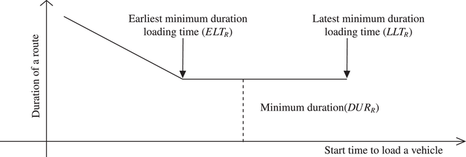
A common service requirement in modern supply chains is to provide a rapid and consolidated delivery of products to customers. Consequently, transportation planning and route creation are given priority over warehouse planning as a timely delivery directly impacts customer experience. Another motivation to prioritize distribution management is that transportation accounts for a large part of a company's logistics costs. According to Rodrigue (2020), these costs account for up to 58% whereas the cost of operating and maintaining warehouses and inventory constitutes around 34%. Such a sequential approach of imposing transportation plans on the operational planning in warehouses relies on warehouse managers being able to process and prepare orders such that vehicles can be loaded and dispatched from the warehouse at their scheduled time. When order delivery due times are longterm (e.g., multiple days), the traditional approach of decomposing the transportation planning from the warehouse operations is sufficient. However, short lead times, often in combination with tight delivery time windows, are common service requirements in modern supply chains such as e‐commerce deliveries (Dayarian & Savelsbergh, 2020), retail store deliveries (Akyol & De Koster, 2013), and shipment consolidations in cross‐dock facilities (Dellaert et al., 2018). The strict vehicle routing schedules and short lead times prevent warehouse managers from efficiently executing the order picking process. In particular, the batch sizes for order picking become smaller, which requires more order pickers and increases the labor cost of manual order picking. Another reason why warehouse managers struggle to easily absorb and accommodate varying routing needs without additional financial burden is that they do not have sufficient capacity at their disposal. A recent survey of warehouse managers found that warehouse space availability is the greatest concern for 43% of the respondents (Turner & Townsend, 2021). In particular, warehouse space is severely scarce in Western Europe, parts of Asia, and coastal regions in North America. The size of the staging space, which serves as a consolidation point for orders before they are loaded onto vehicles, can be a fraction of the daily warehouse output. In grocery retail warehouses, this ratio is usually less than 30%. As a result, the vehicle routing plans result in time periods during which the staging space is fully occupied. This leads to planning disruptions as order picking operations have to be halted and vehicles have to be loaded and dispatched before additional items can be sent to the staging area (Ostermeier et al., 2022). The interactions between the warehouse processes and transportation planning are visualized in Figure 1.

FIGURE 1

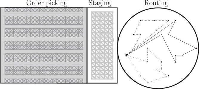
Warehousing and transportation processes considered in this paper.

Most studies in the literature follow the sequential planning paradigm from practice, where the scheduling of vehicle routes ignores any internal warehouse constraints and only focuses on the (timely) distribution of products between the warehouse and delivery locations either computationally (Laporte, 2009) or empirically (Akyol & De Koster, 2013). In contrast, we develop an integrated planning approach where vehicle routes are constructed while considering the most important operational warehouse processes (i.e., batching orders and scheduling order pickers) and satisfying any staging space constraints. Only a few papers use a similar approach. Schubert et al. (2018) are the first to integrate VRP and order picking. The authors minimize the total tardiness of all customer orders where vehicles can only depart from the warehouse once all items of the orders to be delivered by the vehicle have been picked. Orders can only be picked one by one, and a fixed number of order pickers start at the beginning of the planning horizon. Around the same time, Moons et al. (2018, 2019) developed another integrated problem formulation with hard delivery time windows (instead of only a soft delivery due date) and a more general objective function, where they minimize the sum of the travel cost (i.e., number of vehicles), vehicle employment cost (i.e., travel distance), and order picking cost (i.e., number of order pickers). Schubert et al. (2021) extend a similar formulation with a heterogeneous fleet. All aforementioned papers assume a single‐order picking policy, that is, orders are picked one by one, and no staging space limitations. Kuhn et al. (2021) extend the original problem formulation of Schubert et al. (2018) by including a fixed set of possible order batches that can be assigned to the order pickers. Note that this formulation has no cost associated with the ordering picking or vehicle routing decisions. The only paper that includes restrictions on the number of items that can be stored between the order picking and routing processes is by Ostermeier et al. (2022). In their problem formulation, the items of each order need to be picked from different zones in the warehouse (i.e., as suborders) and the space required for the full order is reserved from the moment the first items from a suborder have been picked until the full order has been loaded in the vehicle. This means that the picking of any suborder can only start if sufficient capacity is available at the staging space for the full order (not just the suborder). Similar to other papers, suborders are picked one at a time (i.e., no batching is allowed). Furthermore, the number of order pickers is predetermined instead of a decision variable. We extend all these integrated problem formulations in three ways: (i) order batching is allowed, (ii) multiple shifts of order pickers can start at different points in time over the planning horizon and the number of order pickers in each shift is a decision variable, (iii) the available staging space is restricted but does not prevent the order pickers from starting the picking process (they might have to wait until sufficient space is available at the staging area to drop off the order batch that is picked). We include hard time window constraints for the deliveries and a homogeneous fleet. However, the solution technique developed in this paper can also handle problem formulations where these two assumptions are relaxed.

Our integrated problem formulation is inspired by the operational characteristics as observed by a leading grocery retailer in the Netherlands (see Section 6 for more details). We aim to compare the performance and costs of our integrated approach to other intervention mechanisms that logistics managers can employ when the staging space becomes overwhelmed. The staging process is at the heart of the warehouse operations and connects the order picking process to transport routing. Ultimately, the size of the staging area as well as the speed and time epochs at which the staging space can be filled (through order picking) and vacated (through loading vehicles) determine whether the warehouse can feasibly execute the vehicle routing schedule. In our discussions with managers, two distinct interventions were mentioned. First, warehouse managers can add additional staging space, allowing the order picking process to continue without any interruptions and leading to a more efficient execution of order batches and lower order picking cost. However, a staging space expansion can be costly, as the staging space is a valuable piece of real estate in any warehouse as it is located in front of the dock doors and all warehouse flows pass through the staging space. Second, warehouse managers can request transport planners to negotiate different order delivery time windows at the retail locations such that the dispatch time of vehicles is more favorable for the warehouse operations. The impact of these managerial interventions will be analyzed in our case studies at the partner retailer.

The contributions of this study can be classified as methodological and managerial. Methodologically, we contribute to the literature by formulating a general VRP that incorporates order batching, order picker scheduling, staging, and vehicle loading processes at the warehouse. The integration of warehouse processes with vehicle routing is not new to the literature. However, the models in the literature do not capture the key decision‐making aspects in warehouses that truly drive the order picking cost (that includes order batching and scheduling order pickers). Specifically, batching orders significantly adds to the computational complexity of the integrated problem and is therefore not considered in most papers that combine warehouse operations with transportation planning. In particular, we develop a novel expression that accurately approximates batch processing times as a direct function of the batch size. We validate our closed‐form expression with empirical data. This new (and simple) expression allows us to introduce the new problem formulations and solution algorithms that rely on this new expression. We develop exact algorithms to solve these problems with a sequential approach. For the integrated approach, we provide a solution methodology that is based on an adaptive large neighborhood search (ALNS) algorithm that relies on structural results of the order batching expression.

From a managerial perspective, we perform case studies of the operations in two warehouses operated by our partner retailer, one for ambient products and the other for refrigerated products. The case studies not only focus on evaluating the integrated approach but also investigate common managerial interventions when using a sequential planning approach. Our numerical results show that implementing an integrated planning approach outperforms the alternative interventions. With the current staging capacity, an integrated approach can generate around 9% and 11% of cost savings for the ambient and refrigerated warehouse, respectively. These savings can be made by generating vehicle routing plans that accommodate more efficient order batches, which reduces the number of required order pickers. A time window expansion of only 15 minutes can lead to 4–6% cost savings. However, this expansion is challenging as delivery time windows are governed by contracts, for example, with franchisees. In contrast to the expectations of the industry partner, under high utilization of the staging area, we find that (i) a staging space expansion (equivalent to five FTLs) is a better solution compared to 15‐minutes time window expansions under a sequential planning approach and (ii) the reverse holds under an integrated approach. Under medium‐to‐low utilization of the staging area, we find that (i) adopting delivery time windows that are 15 minutes wider is more beneficial than adding additional staging space under a sequential planning approach and (ii) expanding either the staging space or the time windows can add limited benefits under an integrated approach.

The outline of our paper is as follows. Section 2 reviews the relevant literature. Section 3 introduces the description of the problem and notations. Section 4 formulates the VRP and warehouse planning problem as individual problems. Section 5 presents the formulation of the integrated planning problem and an overview of our ALNS algorithm to solve the integrated problem. We describe the warehouse operations and delivery network of the two case studies in Section 6, and we present the results in Section 7. The paper concludes in Section 8 with our managerial insights.

LITERATURE REVIEW

In this section, we provide an overview of three streams in the literature that are relevant to our study: warehouse planning with order picking in batches, VRPs with constraints on the loading capacity, and integrated warehousing and transportation problems.

Warehouse planning with batch order picking

The main functions of a warehouse are receiving, storage, order picking, and shipping items. Warehouse managers focus most of their efforts on optimizing order picking processes as this contributes to the majority of warehousing costs (Richards, 2021). Order picking involves retrieving items from their storage locations and ensuring that the items are ready to be delivered to customers who ordered them. One of the most prominent strategies to improve the order picking performance is order batching (i.e., combining customer orders into picking orders or batches) (Gademann et al., 2001). This section focuses on papers that consider order batching for warehouses with multiple order pickers.

The joint order batching, assignment, and sequencing problem (JOBASP) describes how a set of customer orders is retrieved from the warehouse as efficiently as possible by combining customers orders into single pick routes (order batching), deciding which order picker is assigned to each batch, and in which sequence the batches are picked to ensure that all orders are picked before their due time. Henn (2015) formulates the problem to minimize the total tardiness of all orders and proposes a variable neighborhood search (VNS) algorithm to solve the optimization problem. Matusiak et al. (2017) minimize the total batch execution time (including pick, travel, and setup time), which depends on the skill set of the order picker assigned to the batch. Due times are not included, and therefore, sequencing decisions are not made. The authors develop an ALNS algorithm to find good solutions. Muter and Öncan (2022) do not include any due times for the order picking either. They propose a column generation and VNS algorithm for the problem to minimize the makespan as primary objective and the total travel time as secondary objective. In these papers, the possible order batches are predetermined. As a result, the order picking time of a batch (or travel time within the warehouse) is calculated offline and is an input parameter for the JOBASP.

Zhang et al. (2017) study the creation of batches in the JOBASP. They assume an S‐shaped picking strategy and a random storage assignment, such that the distance of the picking tour of a batch is based on the number of aisles included in the tour. Simple batching and assignment rules are defined to find a solution. When the storage locations of the individual items are included, and the sequence in which items of a pick route are picked is part of the decision‐making, this is referred to as the picker routing problem. Consequently, the order pickers know an exact path through the warehouse to pick all items in the batch and the distance (and processing time) of the corresponding pick route can be determined. The extension of the JOBASP with such routing decisions for the order pickers in the warehouse is called the joint order batching, assignment, sequencing, and routing problem . Ardjmand et al. (2018) include distances between items and develop a hybrid simulated annealing and ant colony optimization algorithm to solve the problem where the makespan is minimized. In contrast, Scholz et al. (2017) use a graph network to represent the pick locations of items and design a variable neighborhood descent (VND) algorithm to minimize the total tardiness. Van Gils et al. (2019) also use a graph network and propose an iterated local search algorithm to minimize the total order picking time subject to due time constraints.

Interestingly, all the above‐mentioned papers assume that the number of order pickers is given and all order pickers are readily available at the start of the planning horizon (and can thus immediately start with their first picking tour). Rijal et al. (2021) extend the JOBASP with an order picker scheduling problem that generates workforce schedules for multiple shifts by assigning and sequencing (predetermined) batches to order pickers while ensuring that the due time windows of orders are respected. In the individual warehouse planner's problem that we develop in Section 4.2, a similar problem is solved with the exception that the possible batches are not predetermined. Instead, we determine the batch sizes that need to be picked by individual order pickers, where the time of a tour to pick the items of a particular batch depends solely on the number of items in the batch (i.e., the batch size) instead of the individual items. Using data analytics, we find a closed‐form expression that accurately approximates the picking time for a batch. Consequently, we only have to keep track of the number of picked items to verify whether all items of an order have been picked. As a result, we can develop an exact algorithm to solve this new formulation of the JOBASP.

VRP with loading capacity

The vehicle routing literature is vast and varied. For a recent overview of VRP with hard time window constraints , we refer to Pecin et al. (2017) and Zhang et al. (2021). Only very few studies have examined VRPs that are constrained by a loading capacity such that a limited number of vehicles can be loaded at the same time. Hempsch and Irnich (2008) consider routing problems where multiple vehicle routes compete for limited resources. This class of problems is called routing problems with inter‐tour resource constraints. For a variety of such problems, Irnich (2008) presents a unified local search procedure based on resource extensions along a giant route representation of a solution, where a giant route represents a sequence of individual routes based on relevant time and space information. For example, the sequence in which vehicles depart from the warehouse can be the order in which routes are represented in the giant route. El Hachemi et al. (2015) formulate an integer programming problem for the transportation of wood, where special machines are required to load wood onto vehicles. Dabia et al. (2019) and Van der Zon (2017) study the same VRP where the number of available dock doors varies over the day, and the capacity to load items in the vehicles depends on the number of employees at the loading docks. Dabia et al. (2019) use column generation to find an optimal solution, whereas Van der Zon (2017) proposes an ALNS to solve larger‐size problem instances where the loading capacities can be exceeded with some penalty. In the same nomenclature, our integrated warehousing and transportation problem can also be classified as a routing problem with inter‐tour resource constraints. However, instead of the limited availability of the resources being given, order picking and staging are separate resources that interact with each other as well as with the vehicle routes.

Integrated warehouse and transportation planning

This section discusses studies that integrate order picking operations with vehicle routing. For a more general overview of the literature on combining decision‐making problems from a warehouse planning perspective, we refer to Van Gils et al. (2018).

Schmid et al. (2013) are the first to propose extending the VRP with order picking as an interesting research opportunity. Since then, a number of publications have addressed this integrated problem. Two types of objective formulations are considered in the literature: minimizing the tardiness or makespan with soft (or no) delivery time window constraints or minimizing the order picking and delivery cost with hard time window constraints. Schubert et al. (2018) and Kuhn et al. (2021) minimize the total tardiness of all customer orders. The orders are picked one by one (i.e., no batching) in Schubert et al. (2018), who develop an iterated local search algorithm where the initial solution is generated by solving the VRP first with simple rules and then the order picking is determined, and a VND procedure is used for solution improvements. Kuhn et al. (2021) extend the problem formulation with order batches that can be assigned to order pickers and use an ALNS algorithm to solve the problem. Zhang et al. (2018) minimize the makespan and number of vehicle routes since the route planning is simplified with a fixed cost and time duration per route. Consequently, there are no due times or delivery time windows, no sequencing decisions, and the transportation problem is not a VRP. The authors mainly focus on the order picking process where order batching is allowed.

A more general objective function expresses the minimization of the total costs, which consist of travel cost (i.e., number of vehicles), vehicle employment cost (i.e., travel distance and/or time), and order picking cost (i.e., number of order pickers). Such a problem setting was first studied by Moons et al. (2018, 2019). In their work, a fixed number of permanent order pickers are available over the entire planning horizon and temporary order pickers can be hired. Since orders can only be picked one at a time (i.e., order batching is not allowed) and order pickers are paid per minute, the assignment decision of orders to order pickers tries to use permanent order pickers as much as possible since their wage rate is lower. The number of temporary order pickers is not minimized as they are not paid per shift or for a minimum duration. Schubert et al. (2021) set a fixed cost per order picker and consider heterogeneous vehicles that need to satisfy customer requirements (i.e., the assigned vehicle is customer dependent). The authors propose a VNS metaheuristic with a VND algorithm as the local search procedure. Chen et al. (2022) minimize the completion time of picking order batches and travel cost, but they do not include order pickers in their problem formulation. The time to pick items in a batch is determined as in Zhang et al. (2017). The only paper that includes a limited intermediate storage area is by Ostermeier et al. (2022). However, the authors make simplified assumptions about how to use the staging area, which restricts an efficient utilization of the space (see Section 1). Furthermore, a fixed number of order pickers are available. Their solution approach is based on the same techniques as those developed by Schubert et al. (2021). As discussed in Section 1, we extend these references by including decisions regarding order batches, the number of order pickers assigned to shifts, and utilizing a limited staging space while solving the VRP with time windows.

PROBLEM DESCRIPTION AND NOTATIONS

In this section, we discuss the details of the problem and we present a model formulation of the problem.

Topology

The network of a warehouse and all customer locations is represented by graph

$G=(\mathcal{V},A)$

, where

$\mathcal{V}$

indicates the set of vertices and A the set of arcs. A set of n customer locations is indicated by the vertices

${\mathcal{V}}_c:=\{1,2,\cdots ,n\}$

. The warehouse is represented by node 0 to indicate vehicle departures from the facility and by node

$n+1$

to indicate vehicle returns to the warehouse. The complete set of locations is represented by the set

$\mathcal{V}:=\{0\}\cup {\mathcal{V}}_c\cup \{n+1\}$

.

Delivery resources and process

At the start of the planning horizon, customer

$i\in {\mathcal{V}}_c$

demands a total of

$q_i$

units of products. A unit refers to a standardized unit load shipment equipment such as a pallet or roll cage. Identical delivery vehicles are represented by a set

$\mathcal{K}$

, and each vehicle has a capacity of Q units. The time window to deliver the units to customer

$i\in {\mathcal{V}}_c$

is denoted by

$[a_i,b_i]$

, where the service (unloading) at that customer must start within this time window. The service time required at location i is indicated by

${\sigma }_i$

. The travel time and travel distance between location i and j are given by

${\tau }_{ij}$

and

$d_{ij}$

, respectively.

Order fulfillment resources and order processing times

In a manual picker‐to‐parts system, human order pickers travel to product locations to pick items. The number of units picked in a single picking route is called the batch size and is denoted by

$b\in \mathcal{B}$

, where

$\mathcal{B}=\{1,\cdots ,B\}$

is the set of possible batch sizes and B is the maximum batch size. The picking time (or processing time) of a batch with b units is indicated as

${\mu }_b^{-1}$

, where

${\mu }_b$

is the picking rate. The set of order pickers is indicated by

$\mathcal{P}=\{1,\text{…},P\}$

, and at most P pickers can be used in the warehouse.

Order staging and dispatching

The staging space is a buffer between the order picking and vehicle dispatching processes (see Figure 1). In many warehouses, the size of the staging area is significantly smaller than the total number of units picked and shipped from the warehouse on a daily basis. If the staging area is completely filled with unit loads, two operational remedies are available. Managers can either postpone the completion of subsequent batches to be picked by temporarily stopping any order picking activities or by assigning larger batch sizes to pickers, or they can start the loading process of vehicles at an earlier time so that units are cleared from the staging area. Both strategies are inefficient but allow for flexible use of the limited staging space. Using order pickers with a nonoptimal efficiency increases warehouse costs. Vacating the staging area earlier increases the duration during which vehicles are used and consequently raises transportation costs. In our paper, the warehouse has a limited staging capacity of Z units at any time.

Order batching

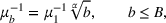
Picking orders in batches is common practice in B2C warehouses. However, customer orders can consist of hundreds of products in B2B retail settings and multiple order pickers need to pick units in parallel to complete one customer's order in time. In such environments, particularly in retail, order batches consist of multiple load carriers (e.g., pick pallets, roll cages) to be picked simultaneously by one order picker. For example, in our case company, order pickers typically use up to five roll cages in the same pick route, where each roll cage can be associated with a different store order. Therefore, it is prohibitively difficult to determine order batch processing times (Gademann et al., 2001). It is more reasonable to use approximate order picking times. Such an approach is taken by Çeven and Gue (2015). They propose a processing rate that is linear in the number of units to pick, that is,

${\mu }_b^{-1}=b{\mu }_1^{-1}$

. This allows for splitting the order (and even a unit) over multiple order pickers, which requires consolidation after picking. However, their expression fails to capture the benefit of batch picking. In practice, the batch processing time per unit decreases with an increase in batch size, that is,

${\mu }_{b+1}^{-1}/(b+1)<{\mu }_b^{-1}/b$

. Therefore, we propose an alternative expression to define the order picking time of a batch, which relies on nondivisible unit picking. This is introduced in Claim 1. Claim 1

The processing time to pick a batch with a size of b units is given by

1

where

$\alpha >1$

is the batch processing time factor.

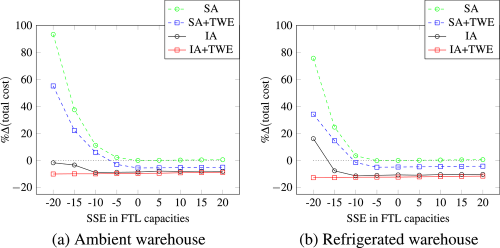
Claim 1 is supported with empirical data from a large retailer in the Netherlands (see Section 6 for more details). The data comprise 4 weeks of information on the orders from individual retail stores, the composition of order batches, the number of units in each batch (i.e., batch size), and the realized processing time of each order batch. A total of 1,086,275 units were picked in 232,000 batches at five warehouses that keep a wide range of products over 54 order picking zones. We performed an ordinary least square regression analysis for each zone to find the best value of the batch processing time factor α (i.e., the value that minimizes the squared error).

Figure 2 shows the distribution of the different α values. A larger value of α indicates that more economies of scale can be obtained with batch picking, whereas a value close to one indicates that there are hardly any efficiencies with batch picking. The average value of R ² associated with the regression analysis is 0.95 with a standard deviation of 0.04. As a result, we conclude that Equation (1) accurately predicts the processing time of a batch with b units.

FIGURE 2

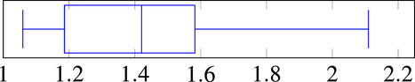
Values of the batch processing time factor α over the 54 picking zones.

Order picker schedule

Order pickers are scheduled in shifts. A shift of type

$h\in H$

(or shift h in short) starts at time

$T_{begin}^h$

and ends at time

$T_{end}^h$

. The binary variable

$u_p^h$

indicates if order picker p is assigned to shift h. The actual schedule of an order picker consists of a sequence of batches assigned to the order picker with positions that specify the order in which the batches have to be picked. In other words, the entire batch in position s is picked before any items of the batch in position

$s+1$

are picked by the same order picker. The binary variable

$y_{pb}^s$

indicates if a batch of b units is assigned to picker p in the

$s\text{th}$

position of the schedule. The Gantt chart in Figure 3 shows an example of the schedule for two order pickers, where three batches are assigned to each order picker. The first order picker is assigned a batch with three units in the first position (i.e.,

$y_{13}^1=1$

). The second order picker is assigned a batch with one unit in the first position (i.e.,

$y_{21}^1=1$

). The later start of the second picker indicates a separate shift.

FIGURE 3

A Gantt chart to illustrate order picker schedules (i.e., variable

$y_{pb}^s$

).

Objective

From a transport planner's perspective, the aim is to minimize the cost associated with the travel distance and the duration that vehicles are used. This usage duration starts when units are loaded into the vehicle, and it ends when the vehicle returns to the warehouse after completing the delivery route. From a warehouse manager's perspective, the aim is to minimize the number of order pickers required to pick the units and place them in the staging area so that vehicles can be loaded on time. The cost of a vehicle (with driver) is c ₁ per unit of time, and the travel cost is c ₂ per unit of distance. The cost of scheduling an order picker in the planning horizon is c ₃.

A summary of the notations for all input parameters and decision variables (including simplifying notations) is presented in Tables 1 and 2, respectively.

TABLE 1

Notations for the input parameters of the integrated warehousing and transportation problem.

Vehicle routing parameters
${\mathcal{V}}_c$	set of customer locations
$\mathcal{V}$	set of customer locations and the warehouse
$\mathcal{A}$	set of arcs
$\mathcal{K}$	set of vehicles
${\sigma }_i$	service time at customer location $i\in {\mathcal{V}}_c$
${\tau }_{ij}$	travel time between locations $i\text{and}j\in \mathcal{V}$
$d_{ij}$	travel distance between locations $i\text{and}j\in \mathcal{V}$
$a_i$	earliest start of the service time at customer location $i\in {\mathcal{V}}_c$
$b_i$	latest start of the service time window at customer location $i\in {\mathcal{V}}_c$
$q_i$	number of units ordered by customer location $i\in {\mathcal{V}}_c$
Q	capacity of a vehicle
c 1	cost of using a vehicle per unit time
c 2	cost of using a vehicle per unit distance

Warehouse parameters
$\mathcal{P}$	set of order pickers that can be used, $\mathcal{P}=\{1,\cdots ,P\}$
$\mathcal{B}$	set of possible batch sizes in the number of units that can be picked in a single batch, $\mathcal{B}=\{1,\cdots ,B\}$
$\mathcal{S}$	set of picking positions
$\mathcal{H}$	set of order picker shift types
$T_{begin}^h$	starting time of shift $h\in H$
$T_{end}^h$	ending time of shift $h\in H$
${\mu }_b^{-1}$	time needed to pick a batch with b units, where ${\mu }_b^{-1}:={\mu }_1^{-1}\sqrt[\alpha ]{b}$
Z	maximum number of units that can be physically located in the staging area at any time
c 3	cost of using an order picker in the planning horizon

TABLE 2

Notations for the decision variables of the integrated warehousing and transportation problem (including simplifying notations).

Decision variables
$x_{ij}^k$	1 if vehicle k travels along arc $(i,j)\in \mathcal{A}$ , 0 otherwise
$l^k$	start time to load vehicle $k\in \mathcal{K}$
$t_i^k$	start time of order delivery at node $i\in {\mathcal{V}}_c$ by vehicle $k\in \mathcal{K}$
$w^k$	number of units available at the staging area when the loading of vehicle $k\in \mathcal{K}$ starts
$y_{pb}^s$	1 if order picker p picks a batch of b units in the $s\text{th}$ position of its schedule, 0 otherwise
$z_{pk}^s$	1 if the batch in the $s\text{th}$ position of the schedule for order picker p is picked before the loading of vehicle k starts, 0 otherwise
$o_p^s$	completion time of the batch in the $s\text{th}$ position of the schedule for order picker p
$u_p^h$	1 if order picker p is assigned to shift type $h\in H$ , 0 otherwise

Simplifying notations
${\delta }^{+}(i)$	set of arcs emerging from node i
${\delta }^{-}(i)$	set of arcs incoming to node i
$x{({\delta }^{+}(i))}^k$	:= $\sum _{j\in \mathcal{V}}{x}_{ij}^k$
$x{({\delta }^{-}(i))}^k$	:= $\sum _{j\in \mathcal{V}}{x}_{ji}^k$
$q(k)$	:= $\sum _{i\in {\mathcal{V}}_c}{q}_{i}x{({\delta }^{+}(i))}^k$

SEQUENTIAL PLANNING

In the literature and in practice, it is common to solve the warehousing and transportation problems sequentially (see Section 1). When the transportation problem is solved first, the times that the units have to be loaded in the vehicle specify the due times for the order picking process in the warehousing problem (see Section 2.1). When the warehousing problem is solved first, the times that the picking of an order is complete specify the earliest time a vehicle can load and dispatch the units in the transportation problem. This is called the release date or ready time of a customer order in vehicle routing. (See Cattaruzza et al., 2016, Reyes et al., 2018, Shelbourne et al., 2017, and Wölck and Meisel, 2022, for recent references.) This section presents the individual subproblems in a sequential approach, where the transport planner's problem is solved first and the warehouse planner's problem second. This is consistent with most observations in practice, including our case studies.

Transport planner's problem

The transport planner's problem is formulated as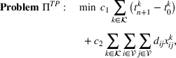

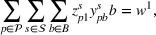
$$\begin{array}{c}\hfill \mathbf{Problem}{\mathrm{\Pi }}^{TP}:\min c_1\sum _{k\in \mathcal{K}}\left(t_{n+1}^k-t_0^k\right)\\ \hfill +c_2\sum _{k\in \mathcal{K}}\sum _{i\in \mathcal{V}}\sum _{j\in \mathcal{V}}{d}_{ij}{x}_{ij}^k,\end{array}$$

2

subject to

$$\begin{array}{c}\hfill \sum _{k\in K}x{({\delta }^{+}(i))}^k=1\forall i\in {\mathcal{V}}_c,\end{array}$$

3

$$\begin{array}{c}\hfill x{({\delta }^{+}(0))}^k=x{({\delta }^{-}(n+1))}^k=1\forall k\in \mathcal{K},\end{array}$$

4

$$\begin{array}{c}\hfill x{({\delta }^{+}(i))}^k=x{({\delta }^{-}(i))}^k\forall i\in {\mathcal{V}}_c,k\in \mathcal{K},\end{array}$$

5

$$\begin{array}{c}\hfill t_i^k+{\sigma }_i+{\tau }_{ij}\le t_j^k+M(1-x_{ij}^k)\forall (i,j)\in \mathcal{A},k\in \mathcal{K},\end{array}$$

6

$$\begin{array}{c}\hfill a_i\le t_i^k\le b_i\forall i\in {\mathcal{V}}_c,k\in \mathcal{K},\end{array}$$

7

$$\begin{array}{c}\hfill q(k)\le Q\forall k\in \mathcal{K},\end{array}$$

8

$$\begin{array}{c}\hfill x_{i,j}^k\in \{0,1\}\forall (i,j)\in \mathcal{A},k\in \mathcal{K},\end{array}$$

9

$$\begin{array}{c}\hfill 0\le t_i^k\forall i\in \mathcal{V},k\in \mathcal{K}.\end{array}$$

10

The objective in Equation (2) is to minimize the cost of the travel distance and duration that vehicles are occupied for loading and transporting customer orders. These periods include any potential wait times before a vehicle can unload and deliver the units within the designated time window specified by the customer order. Constraints (3) ensure that each customer node i is visited exactly once. Constraints (4) and (5) serve as flow conservation constraints: each vehicle k has to leave and return to the warehouse, and if a vehicle k arrives at node i, it also has to leave node i, respectively. Units can only be delivered at node j after the delivery at node i is completed by the same vehicle k (i.e., the previous customer in the delivery route) plus the travel time between the two customer locations by constraints (6), and the delivery should occur within the specified time window according to constraints (7). The number of units delivered in a route cannot exceed the loading capacity of a vehicle k based on constraints (8). Constraints (9) and (10) indicate the domain of the decision variables for the routing problem. The transport planner's problem

${\mathrm{\Pi }}^{TP}$

can be reformulated as a set covering problem and solved using a branch‐and‐price algorithm. (See Appendix EC.1 in the Supporting Information for the details.)

Warehouse planner's problem

The solution to problem

${\mathrm{\Pi }}^{TP}$

specifies the time

$l_k$

when vehicle

$k\in \mathcal{K}$

is loaded, and the number of unit loads

$q(k)$

dispatched by vehicle

$k\in \mathcal{K}$

. The objective of the warehouse manager is to schedule a minimum number of order pickers to have

$q(k)$

units picked at time

$l_k$

for each vehicle

$k\in \mathcal{K}$

while satisfying the operational constraints of the warehouse. The warehouse planner's problem is formulated as

$$\begin{array}{c}\hfill \mathbf{Problem}{\mathrm{\Pi }}^{WP}:\min c_3\sum _{h\in \mathcal{H}}\sum _{p\in P}{u}_p^h,\end{array}$$

11

subject to

$$\begin{array}{c}\hfill \sum _{b\in \mathcal{B}}{y}_{pb}^s\le 1\forall p\in \mathcal{P},s\in \mathcal{S},\end{array}$$

12

$$\begin{array}{c}\hfill o_p^1\ge \sum _{h\in \mathcal{H}}{T}_{begin}^h{u}_p^h+\sum _{b\in \mathcal{B}}{y}_{pb}^1{\mu }_b^{-1}\forall p\in \mathcal{P},\end{array}$$

13

$$\begin{array}{c}\hfill o_p^s\ge o_p^{s-1}+\sum _{b\in B}{y}_{pb}^s{\mu }_b^{-1}\forall p\in \mathcal{P},s\in \mathcal{S}\setminus \{1\},\end{array}$$

14

$$\begin{array}{c}\hfill o_p^{|\mathcal{S}|}\le \sum _{h\in \mathcal{H}}{T}_{end}^h{u}_p^h\forall p\in \mathcal{P},\end{array}$$

15

$$\begin{array}{c}\hfill l^k-o_p^s\le M{z}_{pk}^s\forall k\in \mathcal{K},p\in \mathcal{P},s\in \mathcal{S},\end{array}$$

16

$$\begin{array}{c}\hfill l^k-o_p^s\ge M(z_{pk}^s-1)\forall k\in \mathcal{K},p\in \mathcal{P},s\in \mathcal{S},\end{array}$$

17

18

$$\begin{array}{c}\hfill \sum _{p\in \mathcal{P}}\sum _{s\in \mathcal{S}}\sum _{b\in \mathcal{B}}{z}_{pk}^s{y}_{pb}^{s}b-\sum _{k^{\prime }=1}^{k-1}q(k^{\prime })=w^k\forall k\in \mathcal{K}\setminus \{1\},\end{array}$$

19

$$\begin{array}{c}\hfill q(k)\le w^k\forall k\in \mathcal{K},\end{array}$$

20

$$\begin{array}{c}\hfill w^k\le Z\forall k\in \mathcal{K},\end{array}$$

21

$$\begin{array}{c}\hfill M\sum _{h\in \mathcal{H}}{u}_p^h\ge \sum _{b\in \mathcal{B}}{y}_{pb}^1\forall p\in \mathcal{P},\end{array}$$

22

$$\begin{array}{c}\hfill w^k,l^k\ge 0\forall k\in \mathcal{K},\end{array}$$

23

$$\begin{array}{c}\hfill z_{pk}^s\in \{0,1\}\forall p\in \mathcal{P},k\in \mathcal{K},s\in \mathcal{S},\end{array}$$

24

$$\begin{array}{c}\hfill u_p^h\in \{0,1\}\forall p\in \mathcal{P},h\in \mathcal{H},\end{array}$$

25

$$\begin{array}{c}\hfill y_{pb}^s\in \{0,1\}\forall p\in \mathcal{P},b\in \mathcal{B},s\in \mathcal{S},\end{array}$$

26

$$\begin{array}{c}\hfill o_p^s\ge 0\forall p\in \mathcal{P},s\in \mathcal{S}.\end{array}$$

27

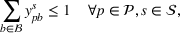
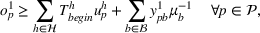
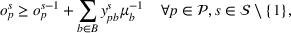
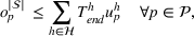
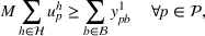
The objective in Equation (11) minimizes the total order picking cost. Constraints (12) allow each picking position to be used at most once for each order picker. Constraints (13) and (14) determine the time when the picking of the order batch at a specific picking position assigned to an individual order picker is completed. Constraints (13) and (15) ensure that the ordering picking is performed during the shift assigned to the order picker. Constraints (16) and (17) track which picking positions and the associated batches are completed before the loading of a vehicle starts. Note that the variables

$z_{pk}^s$

indicate whether order picker p completes picking the units for the

$s\text{th}$

‐order batch before the loading process starts for vehicle k, regardless of whether these units have to be loaded into vehicle k. Constraints (18) and (19) determine the number of unit loads available at the staging area when vehicle k is loaded. Constraints (20) ensure that vehicles can only start loading after all units requested by the customers for the delivery route of that vehicle are available at the staging area. Constraints (21) impose the capacity limitation of the staging area on the number of items that can be picked and staged at any time. Constraints (22) identify which order pickers are used. Constraints (23)–(27) define the domain of the decision variables associated with the order picking and staging processes.

It can be argued that constraints (20) are somewhat restrictive as we could also consider loading units in a vehicle once parts of these units are available at the staging area for a delivery route. We do not allow for such flexibility for three main reasons. First, it would significantly increase the number of alternatives in any solution procedure, which increases the computational complexity to find a good solution within a reasonable computational effort. Second, vehicles would be located at the loading dock longer, which raises the cost associated with transportation (i.e., the cost for truck drivers as well as occupying trailers). Third, in many warehouses, all pallets or roll cages destined for a single customer need additional checking for completeness before being loaded in a vehicle. However, we do allow for early departures of vehicles, which can be seen as a similar trade‐off as the early loading of units in vehicles. Both alternatives provide more flexibility for order picking and the use of the available staging space at the expense of using the vehicles longer. Furthermore, the problem formulation already allows for shorter routes to load units earlier in vehicles, which comes at the expense of additional routes to the transportation planning. Please note that constraints (18) and (19) are nonlinear. As the nonlinear term contains one binary variable, it can be easily made linear following the linearization procedure in Glover (1975).

Structural properties of warehouse planner's problem

We present the following proposition for the complexity of the warehouse planner's problem. Proposition 1

Even with fixed routes and departure times (i.e., for given values of

$x_{ij}^k$

,

$l^k$

, and

$q_k$

) and a fixed number of order pickers, the problem of finding a feasible batch schedule is NP‐hard.

Proof 1

See Appendix EC.2 in the Supporting Information.

$\square$

Lemma 1

The maximum order picking throughput of an individual picker within a duration of t time units is given by

$$\begin{array}{c}\hfill f(t)=\sum _{b\in \mathcal{B}}{n}_b(t)b,\end{array}$$

28

where the number of batches of size b equals

29

Note that

$n_b(t)\in \{0,1\}$

for

$b\in \mathcal{B}\setminus \{B\}$

and

${\sum }_{b\in \mathcal{B}\setminus \{B\}}{n}_b(t)\le 1$

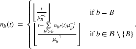
. Lemma 1 follows directly from the fact that batch processing times in Equation (1) are concave decreasing (i.e., the first‐order derivative is positive and the second‐order derivative is negative). Theorem 1

The maximum order picking throughput for the batch picking time in Equation (1) is superadditive, that is,

$$\begin{array}{c}\hfill f(t_1+t_2)\ge f(t_1)+f(t_2).\end{array}$$

30

Proof 2

Consider the order picking throughput during two separate time segments with a duration of t ₁ and t ₂ time units as

$f(t_1)={\sum }_{b\in \mathcal{B}}{n}_b(t_1)b$

and

$f(t_2)={\sum }_{b\in \mathcal{B}}{n}_b(t_2)b$

, respectively. As mentioned above, there exists at most one

$b^{\prime }\in \{1,\cdots ,B-1\}$

such that

$n_{b^{\prime }}(t_1)=1$

and at most one

$b^{\prime \prime }\in \{1,\cdots ,B-1\}$

such that

$n_{b^{\prime \prime }}(t_2)=1$

. If the two separate time segments are combined into one time segment with a duration of

$t_1+t_2$

time units, the first

$n_B(t_1)+n_B(t_2)$

batches of B units are picked in the same amount of time. The time to pick the remaining

$b^{\prime }+b^{\prime \prime }$

units is shorter than if the units were picked separately, because the batch processing time in Equation (1) is concave decreasing.

$\square$

The warehouse planner's problem can be reformulated as a set covering problem (see Appendix EC.3 in the Supporting Information) and solved using a branch‐and‐price framework. The pricing problem for this problem is new to the literature. (See Appendix EC.4 for more details in the Supporting Information.)

INTEGRATED PLANNING

In the integrated problem formulation, the sum of the transportation and warehousing cost is minimized under the same constraints as defined in the previous section: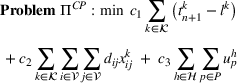

$$\begin{array}{c}\hfill \mathbf{Problem}{\mathrm{\Pi }}^{CP}:\min c_1\sum _{k\in \mathcal{K}}\left(t_{n+1}^k-l^k\right)\\ \hfill +c_2\sum _{k\in \mathcal{K}}\sum _{i\in \mathcal{V}}\sum _{j\in \mathcal{V}}{d}_{ij}{x}_{ij}^k+c_3\sum _{h\in \mathcal{H}}\sum _{p\in P}{u}_p^h\end{array}$$

31

subject to constraints (3)–(10) and (12)–(27).

We develop an ALNS algorithm to solve the integrated optimization problem. The proposed procedure is a decomposition algorithm consisting of three subroutines that are executed iteratively. Routes and a vehicle loading sequence are generated in the first subroutine, the actual start times when vehicles are loaded in the second, and the order picker schedule in the third. The complete pseudo‐code and parameter settings for the ALNS procedure (including how to generate an initial solution and an appropriate stopping criterion) are presented in Appendix EC.5 in the Supporting Information. In the remainder of this section, we only present the salient features of the subroutines that are unique to the problem under study. In particular, the second subroutine GLT is described in more detail as it captures a new approach to include order batching that relies on Theorem 1.

Generation of routes and loading sequence (subroutine GR_LS)

We use the giant route representation proposed by Irnich (2008) to show the sequence of routes arranged in ascending order when the associated vehicles start their loading process at the warehouse. An example of a giant route representation for a solution of eight customer locations and three routes is presented in Figure 4. Zero indicates a vehicle departure from the warehouse, 9 is a vehicle returning to the warehouse, and

$\stackrel{\sim }{0}$

separates individual routes. The route that is loaded first at the warehouse visits the customers at nodes 3‐7‐6, etc. Subroutine GR_LS uses destroy and repair operators to alter the composition of routes and their sequences in the giant route. Details about the individual operators are presented in Appendix EC.5 in the Supporting Information.

FIGURE 4

A giant route representation of eight customer locations visited in three routes.

Generation of loading times (subroutine GLT)

The output of subroutine GR_LS provides a giant route

$\mathcal{R}$

. Let

$R(n)$

indicate the nth route in the giant route

$\mathcal{R}$

. The second subroutine sets the start times of loading units in a vehicle for each route

$R(n)\in \mathcal{R}$

, denoted by

$T_{R(n)}^{Loading}$

. This is done based on backward propagation and the results from Theorem 1. In particular, two mechanisms play a major role in setting these loading times.

The first mechanism is creating and scheduling order batches to be picked. Remember that Theorem 1 specifies that combining order picking of two smaller time segments into one larger time segment is more efficient. Consequently, we introduce the concept of full batches, which are batches that consist of B units to pick. These are the most efficient batch sizes. Any batches of size

$b<B$

are referred to as less‐than‐full batches. Subroutine GLT starts by planning the picking of full batches for route

$R(n)$

as long as sufficient time is available. These are scheduled to be picked at the end of the picking sequence for an order picker. Smaller‐sized batches are scheduled to be picked at the beginning of an order picker's shift because these less efficient batches can potentially be combined with units that are necessary for a route that is loaded earlier (note that these routes are scheduled later with backward propagation).

The second mechanism is identifying the time interval during which the loading of a vehicle for route

$R(n)$

has to start in order for that route to incur the lowest cost. In particular, every route R has a minimum duration denoted by

$DU{R}_R$

, which is the shortest possible duration required for the vehicle to be loaded, serve all the customers in the route, and return to the warehouse. The route can be completed in

$DU{R}_R$

time units if and only if the loading of the vehicle starts within a time interval between the earliest minimum duration loading time (

$EL{T}_R$

) and the latest minimum duration loading time (

$LL{T}_R$

). If loading starts after

$LL{T}_R$

, the vehicle cannot execute route R without violating the delivery time window at one or more customer locations visited in route R. The loading process can also start before

$EL{T}_R$

, but this incurs additional cost as the vehicle has to wait before it can deliver the items at one or more customer locations. These concepts are illustrated in Figure 5. The values of

$EL{T}_R$

and

$LL{T}_R$

depend on the customer locations visited in route R. Therefore, these values are determined dynamically in the solution approach as routes are added to the giant route

$\mathcal{R}$

by adapting the methodology proposed by Tilk and Irnich (2017), who developed it to solve a minimum tour duration problem.

FIGURE 5

Duration cost of a route as a function of the time when the vehicle is loaded.

We now explain how the backward propagation procedure works. It starts with the last route in

$\mathcal{R}$

to depart from the warehouse. To make the most use out of the staging space and the order picking process, it is easy to see that the loading for this route should start as late as possible. The vehicle for the next‐to‐last route R in

$\mathcal{R}$

is ideally scheduled to get loaded at the corresponding

$LL{T}_R$

and so on. However, this may not be possible if the staging space is full. Consequently, the loading of the vehicle has to be scheduled earlier. If this exceeds beyond the corresponding time

$EL{T}_R$

, there will be an additional cost for dispatching the vehicle early. The details about the labels and extension functions to determine

$DU{R}_{R(n)}$

,

$EL{T}_{R(n)}$

,

$LL{T}_{R(n)}$

, and

$T_{R(n)}^{Loading}$

for route

$R(n)$

are presented in Appendix EC.5 in the Supporting Information.

Generation of shift schedules (subroutine GSS)

After completing subroutine GLT, we know when the vehicle for each route

$R\in \mathcal{R}$

is loaded (by

$T_R^{Loading}$

) and the number of units that are in the staging area at that time (denoted by

$Q_R^{FBEnd}$

). Given these values, the column generation algorithm for the warehouse planner's problem can be used to schedule the minimum number of order pickers. However, the increased computational burden of such an exact approach outweighs its benefit in an iterative framework such as the ALNS algorithm. Therefore, we propose a forward propagation procedure that iteratively adds order pickers to each shift to maximize the batch sizes assigned to these order pickers (following the insights from Theorem 1). A detailed pseudocode for subroutine GSS is presented in Appendix EC.5 in the Supporting Information.

DESCRIPTION OF CASE STUDIES

This section provides a detailed description of the cases from one of the leading grocery retailers in the Netherlands that inspired our study. They have six distribution centers (DCs) (two national, four regional), each with their own warehouses for ambient and refrigerated products. We use the two warehouses from the regional DC that supply the retail stores in the northwest region of the country to serve as our case instances for the numerical study in the next section. This region contains 273 store locations. The retailer operates three store formats, which are distinguished by store size. Small stores are located in areas with large daily traffic, such as train stations, airports, and university campuses. Medium‐sized stores are located in cities and residential areas. Large stores are comparable to supermarkets and are often located further away from densely populated city centers.

Store managers place orders in the order management system at least one day in advance. Store orders consist of individual stock‐keeping units, the quantity ordered, and the delivery time window. These orders are translated into several roll cages that are prepared at one of the four regional DCs. Each roll cage will be referred to as a unit in the remainder of this section. Transportation planners create a vehicle routing schedule that includes dispatching times when vehicles have to leave the warehouse, and the warehouse manager has to make sure the items are picked and prepared in units that can be loaded into vehicles before these dispatching times (i.e., a sequential approach). Although the two warehouses serve the same set of store locations, they handle different types of products and have independent delivery routes and picking operations. Furthermore, they have different spatial costs and do not share any staging or picking resources. Table 3 summarizes the case attributes based on 28 days of operational data received from the retailer. We note that the time period over which the data were collected is representative for “normal” operations at both warehouses (i.e., not during a peak season).

TABLE 3

Summary of the operational characteristics of the warehouse with ambient products (case 1) and the warehouse with refrigerated products (case 2).

Component	Attribute	Case 1	Case 2
Delivery network	Average travel time (minutes)	34	34
	Minimum daily deliveries (number of stores)	188	247
	Maximum daily deliveries (number of stores)	356	368
	Average daily deliveries (number of stores)	294	314
	Vehicle capacity (units)	54	54
	Average store drop size (trucks)	0.32	0.32
	Average small store drop size (trucks)	0.12	0.06
	Average medium store drop size (trucks)	0.34	0.34
	Average large store drop size (trucks)	0.4	0.46
	Average unloading time (minutes)	100	100
	Average time window length (minutes)	65	65
Warehouse	Size of staging area (units)	2106	1944
	Minimum daily outputs (units)	3583	4832
	Maximum daily outputs (units)	7013	6492
	Average daily outputs (units)	5180	5412
	Unit picking time (minutes)	13.9	11.7
	Batch processing time factor	1.42	1.65
	Maximum batch size (units)	5	5
	Staging space (€ per square meter per year)	75	75
Costs	Order picking cost (€ per picker per hour)	25	25
	Truck driving cost (€ per truck driver per hour)	25	25
	Truck travel fuel cost (€ per kilometer)	0.36	0.36
	Truck refrigeration cost (€ per hour)	0	3.80
	Staging space rental cost (€ per square meter per year)	75	75
	Staging space energy cost (€ per square meter per year)	3.60	11.90

Delivery network

The data reveal that the travel duration between the warehouses and retail stores ranges between 5 and 104 minutes, with an average duration of around 34 minutes. The size of an order delivery to a retail store is measured in terms of the number of roll cages (or units), which are used to consolidate products. Each roll cage has a standard unit size. Separate sets of vehicles deliver the ambient and refrigerated products to customers. Both types of trucks can hold at most 54 roll cages. There are more frequent deliveries from the refrigerated warehouse. The average drop size of 0.32 truck loads is similar between the two cases, but the average drop size by store format shows interesting differences. The drop size for refrigerated products at small stores is 0.06 and significantly smaller compared to 0.12 for ambient products. These stores have limited refrigerated shelf space and rely on smaller and more frequent deliveries. Figure 6 shows the distribution of drop sizes from both warehouses by store format.

FIGURE 6

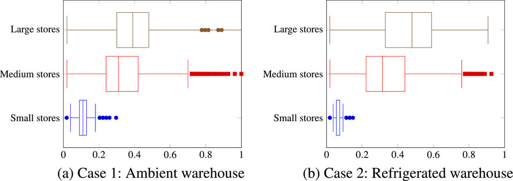
Distribution of the drop size by store format for each case study.

The delivery time window to start service at a store location has an average duration of 65 minutes for deliveries from both warehouses. However, these time windows are usually specified at different times of the day for the same store location. The average service time (or unloading time) at a retail store is around 100 minutes. Figure 7 presents the distributions of the travel time, unloading time, and arrival time window length.

FIGURE 7

Distribution of the delivery network characteristics for each case study.

Warehouse operations

The picking operations at both warehouses start every day at 11 p.m., and the customer locations are visited between 3 a.m. and 8 p.m. Order picking is performed in a low‐level picker‐to‐parts mode at both warehouses. The pick trucks have a capacity of at most five roll cages. Order pickers are scheduled in one of three 9‐hour shifts (starting at 11 p.m., 7 a.m., or 8 a.m., respectively).

The staging area for ambient products can hold 2106 units (or roll cages) at a time, which is equivalent to 39 full truckloads (FTLs). The staging area for refrigerated products is slightly smaller. The maximum number of units with ambient products delivered from the warehouse equals 7013 roll cages, which is almost 10% more than for the refrigerated products. However, the average number of daily deliveries of refrigerated products is higher and has a lower variability in daily outputs.

Order picking of ambient products has longer travel distances because the warehouse has a larger footprint. The unit picking time (i.e., time to pick a batch size of one roll cage) is 13.9 minutes in the ambient warehouse compared to 11.7 minutes in the refrigerated warehouse. Significant efficiency gains can be obtained by batch picking in both warehouses. The refrigerated warehouse has a higher batching efficiency than the ambient warehouse (batch processing factor of 1.65 and 1.42, respectively).

The cost of an order picker is € 25 per hour and is identical to the cost of a truck driver. The travel cost of a heavy semitrailer is around € 0.36 per kilometer regardless of whether the truck is used for ambient or refrigerated products. However, refrigerated products require an additional € 3.80 per hour to power the diesel generator to cool the trailer. To study the impact of expanding the staging space as an intervention mechanism, we need to specify the cost per square meter in the two warehouses. The spatial cost for comparable warehouses in the vicinity of the DC is € 75 per year per square meter (Jones Lang LaSalle IP, 2022). The staging area for one FTL requires a space of 17.6 by 4 meters. After subtracting the required space to maneuver around with order picking equipment, the effective space for the unit loads is 13.6 by 2.45 meters. Consequently, the annual cost of one FTL of staging space equals € 5,280. The annual energy cost is € 3.60 and € 11.90 per square meter for the ambient and refrigerated warehouse, respectively. Details about the energy cost can be found in Appendix EC.6 in the Supporting Information.

RESULTS

This section presents the results of our case studies, where we investigate the impact of three managerial interventions to make the order picking process and vehicle routing more efficient. First, warehouse managers can invest in additional staging space (labeled as staging space expansion or SSE). We consider increasing as well as decreasing the staging space up to 20 FTLs in steps of five FTLs (the current staging capacity at the warehouse for ambient and refrigerated products is 39 FTLs and 36 FTLs, respectively). A positive value for SSE indicates additional staging space, whereas a negative value indicates less space than currently available. We decided to include scenarios where the staging space is reduced by 20 FTLs to represent periods of time in the year where the utilization rates of all capacities (order pickers, staging space, and vehicles) are significantly higher (such as in December). Second, warehouse managers can negotiate less stringent time windows to deliver the replenishment orders at customer locations (labeled as time window expansion or TWE). To study the impact of this intervention, we add an extra 15 minutes to the end of each delivery time window. Third, the warehouse operations and transportation planning can be solved simultaneously instead of sequentially to make better trade‐off decisions between the conflicting objectives as outlined in Section 5 (labeled as integrated approach or IA).

Benchmark solution

The current planning approach to decide on the order picking processes and vehicle routing schedules at the retailer of our case studies will be used as a benchmark (labeled as sequential approach, or SA). In this approach, routes are generated first and the associated vehicle loading times are imposed on the warehouse planning. Next, warehouse managers determine the number of order pickers for each shift that is necessary to have all unit loads available at the staging space before vehicle departure. Table 4 presents the average daily cost and other performance measures for the benchmark solutions (i.e., average over the 28 instances without managerial interventions per case study).

TABLE 4

Average performance of the cost and some operational measures per day for the benchmark solutions.

Performance measure	Case 1	Case 2
Total vehicle routing cost	€ 28,500	€ 32,700
Total order picking cost	€ 24,600	€ 21,200
Number of order pickers scheduled per shift	21/50/39	19/43/33
Number of order batches picked	4,150	3,512
Number of vehicles departing from the warehouse	120	125

In the remainder of this section, we mainly illustrate our results for the case study in the warehouse with refrigerated products and refer to Appendix EC.7 (in the Supporting Information) for the results of the ambient warehouse since the figures have similar patterns.

Impact of managerial interventions on cost

The relative cost comparison between two solutions is presented by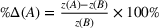

$\%\mathrm{\Delta }(A)=\frac{z(A)-z(B)}{z(B)}\times 100\%$

, where

$z(A)$

and

$z(B)$

denote the total cost corresponding to the solutions A and B, respectively. In all our cost comparisons, the retailer's solution under the current mode of operation (i.e., SA without TWE or SSE) is used as benchmark solution B. Figure 8 illustrates the average relative cost increase based on the total cost when implementing the managerial interventions. Figure 9 presents the average relative changes to the vehicle routing cost and order picking cost for the case study at the refrigerated warehouse. Note that a negative number for

$\%\mathrm{\Delta }(A)$

indicates cost savings. Furthermore, the extra cost for additional staging space under SSE is included in the total cost for intervention A. When the staging space is reduced, the cost savings are deducted from the total cost for intervention A.

FIGURE 8

Impact of managerial interventions (SSE, staging space expansion; TWE, time window expansion; and IA, integrated approach) on total cost in comparison to the retailer's sequential approach (SA) for the ambient and refrigerated warehouse.

FIGURE 9

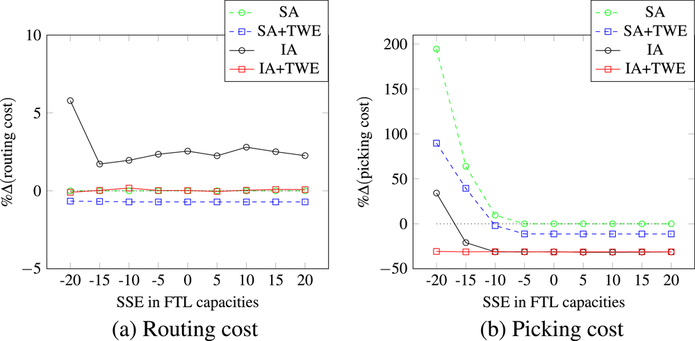
Impact of managerial interventions (SSE, staging space expansion; TWE, time window expansion; and IA, integrated approach) on routing and order picking cost in comparison to the retailer's sequential approach (SA) for the refrigerated warehouse.

Several interesting conclusions can be drawn from these figures when considering the marginal value of the staging space and its interactions with TWE and the choice of the planning approach (i.e., SA or IA). First, increasing the staging space (i.e., without other interventions) does not lead to lower costs. In fact, the total cost increases by 0.6–0.7% for the ambient and refrigerated warehouse, respectively, when 20 FTLs are added to the current staging space. There are no cost savings for the vehicle routing or order picking process. The increase in total cost is caused by acquiring and operating the additional staging space. This contradicts the warehouse managers' expectations that additional staging space alone can lead to greater cost savings and bridge the gap to IA. Note that the results presented here are for a period with “normal” circumstances (i.e., no peak demand). SSE of −5 and −10 FTLs would be representative for periods of increased demand. For “normal” periods, additional staging space under the sequential planning approach is without additional benefit.

Interestingly, we find that the refrigerated warehouse can operate without additional cost when the staging space is reduced by five FTLs. Reducing the staging space beyond five FTLs leads to an exponential increase in total cost for both warehouses, mainly driven by higher order picking costs. Second, expanding the staging space has no additional benefit, not even in combination with any of the other interventions. However, when IA is implemented, reducing the staging space by 10 FTLs has no significant impact on additional ordering picking or vehicle routing costs in either of the two warehouses. The same holds true for a reduction of the staging area by 20 FTLs when both IA and TWE are implemented.

Third, implementing TWE reduces costs by around 5.6% and 4.9% compared to the benchmark solution in the ambient and refrigerated warehouse, respectively. Most of these cost reductions result from a more efficient order picking process as the reduction in routing cost is only 0.75% for both warehouses. When TWE is implemented in combination with SSE, the same conclusions hold (i.e., additional staging space does not result in extra cost reductions). TWE only leads to a lower cost increase when the staging space is reduced by 15 or 20 FTLs. This means that (i) TWE in itself is beneficial regardless of whether there is sufficient staging space and (ii) TWE becomes more beneficial when there is a lack of staging space.

Fourth, whether TWE has a bigger impact than SSE depends on the circumstances. When there is a lack of staging space and the sequential planning approach is used, it is more favorable to increase the staging space rather than to expand the time windows. The reverse observation is made when the integrated approach is used. However, when there is sufficient staging space, then TWE is preferred over SSE.

Fifth, IA is good at balancing between the order picking cost and the vehicle routing cost. The generated vehicle routes result in an average routing cost increase of around 2.5% in both case studies, but the reduction in the order picking cost is more than 20% in the case study for the ambient products and 31% in the case study for the refrigerated products. Overall, the total cost decreases by 8.6% and 10.7% in the ambient and refrigerated warehouse, respectively. Sixth, IA is hardly responsive to the available staging space (or lack thereof). If IA is employed, the staging space can be reduced by 10 FTLs (approximately 26% of the space currently available) without additional cost in both case studies. Even if the staging space is reduced by 20 FTLs, IA can largely mitigate the impact on the order picking cost (which increases exponentially when there is a severe shortage in staging space). In comparison, the total cost increases by only 16% when the staging space reduces by 20 FTLs and IA is employed in the case study with the refrigerated products, whereas the total cost increases by almost 80% otherwise. For the case study with the ambient products, these cost increases are around 0% and almost 94%, respectively. Especially when IA and TWE are employed simultaneously, there is hardly any impact on the total cost when the staging space is reduced by 20 FTLs.

We have validated these results for a set of stylized instances inspired by the case study in the warehouse with ambient products. (See Appendix EC.8 in the Supporting Information.)

Impact of managerial interventions on operational characteristics

This section studies other performance measures to explain the impact of the various managerial interventions at the operational level.

Figure 10 shows the time‐average utilization of the staging space under the different managerial interventions for the refrigerated warehouse. First, we observe that the available staging space is utilized on average only 20% in the benchmark solution. However, the maximum utilization is closer to 62% and the standard deviation of the utilization is around 17%. The profile for the average utilization is very similar when IA is implemented. The average utilization is even slightly higher. However, the standard deviation and maximum utilization decrease with IA. This means that IA makes better use of the space when it is available and tries to avoid scenarios where the utilization becomes too high (i.e., a bottleneck for the order picking process). That being said, implementing TWE greatly reduces the utilization ratio of the staging space (both the average and standard deviation) since more favorable departure schedules and route plans can be designed. This effect is even more pronounced when IA and TWE are implemented simultaneously.

FIGURE 10

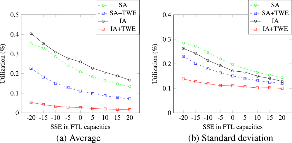
Utilization of the staging space in the refrigerated warehouse.

Other than the use of the available space in the staging area, we also studied the impact on the order picking operations. It is well understood in the warehousing literature that order batching is key to greater efficiency in the picking process (De Koster et al., 2007). Figure 11 confirms that any cost savings through the adoption of each of the three managerial interventions are realized through larger batch sizes per picking tour. The strength of IA is the fact that it makes the order picking process more efficient by increasing the batch sizes: roughly one additional unit load is picked in an order picking route (see Figure 11a). This also explains the higher utilization of the staging space. When changes to vehicle routes are somewhat expensive, larger batch sizes result in a higher utilization of the staging space (i.e., there is less flexibility to synchronize when the order batch is picked and when the picked units are loaded in vehicles for the routing plan). However, there is more flexibility to adjust route compositions and departure times when TWE is employed without compromising the larger batch sizes. Consequently, the utilization of the staging space is greatly reduced with TWE.

FIGURE 11

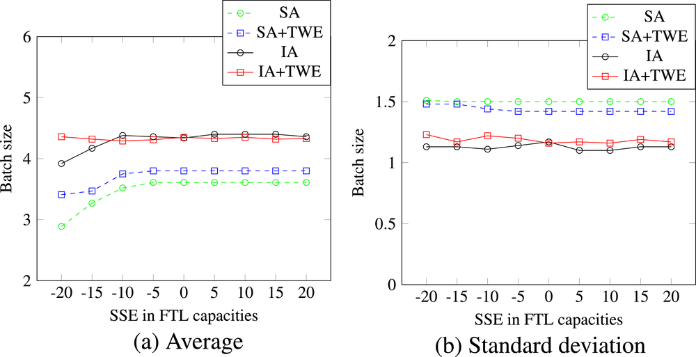
Batch sizes for the refrigerated warehouse.

When we compare the schedules of vehicles departing from the warehouse, we observe that the benchmark solution (i.e., SA) can spread vehicle departures more equally over the planning horizon than IA (when considering the standard deviation of the inter‐departure times). (See Figure 12a.) This is mainly because IA results in larger batch sizes and a lower standard deviation in the batch sizes. Consequently, the departure times of vehicles are more correlated to the start times of the shifts for the order pickers when IA is adopted. Furthermore, larger batch sizes mean that multiple vehicles can get loaded once the order picker drops off the units from the pick tour at the staging area. This also results in periods during which many vehicles depart around the same time. Finally, we also analyzed to what extent vehicles depart early from the warehouse to make space available at the staging area when IA is implemented. Without TWE, this is on average around 23 hours per day, and around 6 hours per dday when TWE is also adopted (as presented in Figure 12b).

FIGURE 12

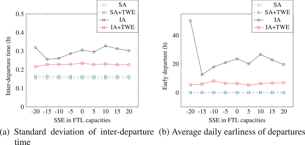
Departure characteristics for the vehicle routes in the refrigerated warehouse.

DISCUSSION AND CONCLUSION

This study investigates the joint planning of warehouse operations and transportation when order deliveries are dictated by time windows. We developed a novel approach to approximate processing times of order picking batches that we incorporated in the scheduling of warehouse personnel and route planning in a computationally tractable manner. Consequently, the integrated problem formulation allows for a better trade‐off between more efficient longer picking routes (i.e., shorter picking time per unit) and more flexible shorter picking routes (i.e., more flexibility regarding the timing when units become available at the staging area, which can be beneficial for transportation planning).

Our two case studies investigated three managerial interventions: adopting an integrated planning approach (IA), expanding the storage space (SSE), and negotiating wider delivery time windows (TWE). From our numerical results, the following managerial insights and practical implications have been derived:

Insight 1: An integrated planning approach outperforms other managerial interventions. IA generates larger cost savings compared to SSE or TWE (individually and jointly). The value of the integrated planning approach (or IA in short) is not limited to only the retail industry, which has been the main focus of this study. Its value is dictated more by the characteristics and conditions of the operational environment rather than the industry attributes. If warehouse resources are limited and delivery deadlines are strict, IA could be valuable to distribution warehouses in other industries such as discrete manufacturing and international spare parts delivery (which also has strict transport due times). Most hub‐and‐spoke distribution networks also require timely deliveries. However, IA will have limited value if shipments are made without hard delivery time windows, such as fluid shipment deliveries where vehicles can depart with picked items at any time epoch. Additionally, when ample staging space is available or the utilization of the staging space does not fluctuate much during the planning horizon (due to spread out vehicle departures), the adoption of IA will have a reduced benefit.

The implementation of IA may face barriers that stem from two sources. First, the enactment of IA requires organizational changes to planning departments for transportation and warehousing which are traditionally kept separate. Such changes may cause employee resistance and disruptions. Second, IA requires additional investments in tailored software implementations that can be prohibitive for small‐ and medium‐sized companies. In contrast, a large number of vendors provide mature software solutions for decomposed problems which are more accessible to small‐ and medium‐sized companies.

Insight 2: Think twice about expanding staging space. Expanding the staging space with 20 FTLs costs less than 1% of the total cost. Managers may be tempted to consider SSE because of its relatively low cost. However, the grocery industry is characterized by an average gross profit margin of as little as 2.5% (BusinessWire, 2022). Our case studies illustrate that SSE is only relevant to consider when the average utilization rate of the staging area over the entire planning horizon is 30% or higher. However, TWE gains more benefits than SSE under IA. Additional staging space can have a significant impact on the bottom line of the company.

In countries with lower real estate and energy costs, staging space expansions could be less cumbersome. Furthermore, if yard space is available and trailers can be used without earliness cost (e.g., when trailers are owned by the company itself), loading trailers in advance is analogous to increasing staging space albeit with some additional material handling cost. If space is not available within the existing warehouse structure or yard space is not available, a physical expansion of the warehouse is necessary which can be more expensive. In any case, our results show that the benefits can be limited and, therefore, caution should be warranted.

Insight 3: Modest time window expansions are valuable in sequential planning approaches. As shown in our case studies, expanding time windows has limited benefits under IA. In contrast, TWE leads to more favorable dispatch schedules under a sequential planning approach, which leads to significant reductions in the routing cost and order picking cost. However, TWE can be difficult to arrange especially when stores are franchised and delivery times are governed by contracts. Store managers may also resist TWE as repeated changes to delivery times at stores disrupt shelving times of products and interfere with periods of high customer traffic.

Insight 4: Route planners should provide warehouse managers with alternative transportation schedules. In practice, to the best of our knowledge, transport planning departments provide only one route and dispatch plan to warehouse managers. Most commercial routing solvers that use either heuristics or exact algorithms, already generate multiple “good” solutions which can easily be extracted and shared with warehouse planners. Designing order picking operations for different vehicle dispatching schedules can lead to substantial savings in warehousing cost. However, the suggested change may face resistance from transportation planners as it may adversely affect the performance indicators that judge their performance. To overcome this barrier, retailers can adopt a welfare‐sharing mechanism between the two departments or judge the overall cost performance. However, the cost savings in this suggested sequential approach with multiple routing schedules can be highly coincidental as this approach lacks an iterative improvement mechanism to guide the selection of routing schedules that make the order picking process more efficient.

Footnotes

ORCID

René de Koster

Supplementary Material

Please find the following supplemental material available below.

For Open Access articles published under a Creative Commons License, all supplemental material carries the same license as the article it is associated with.

For non-Open Access articles published, all supplemental material carries a non-exclusive license, and permission requests for re-use of supplemental material or any part of supplemental material shall be sent directly to the copyright owner as specified in the copyright notice associated with the article.

0.00 MB

0.56 MB