Multiperiod channel coordination in franchise networks: The necessity of internal inventory trading and franchiser involvement

Abstract

Facing consumers' growing demand for fast order fulfillment, it is important yet challenging for franchise companies to best incentivize frequent inventory sharing among their independent franchise retailers or dealers to achieve channel coordination. Past literature has only addressed such channel coordination for one‐time inventory sharing using contractual agreements, which unfortunately do not work for frequent inventory sharing. In this study, we consider multiple inventory‐sharing opportunities and propose a novel coordinating mechanism: internal inventory trading, enabled by disruptive IT platforms, such as the OneView platform's Inventory Management module (OVIM). On the OVIM, designed and operated by a brand (franchiser), every retailer (franchisee) can frequently access to all brand inventories virtually as they trade (buy or sell) inventory with one another and the brand. Using dynamic multiperiod games, we investigate how the brand should craft the trade rules and how the retailers should respond and trade periodically in equilibrium. We prove that channel coordination can be achieved in equilibrium, and the coordination requires both an internal inventory‐trading platform and the brand's proactive involvement in trading as the rule and market maker. Specifically, the coordinating trade rules require the brand to (1) only profit from the royalties (not from trading), (2) set the coordinating trade prices (CTPs) to respond to the real‐time channel inventory, and (3) let the buyer and the seller split shipping costs in any proportion, but not offering any subsidy. We provide a detailed characterization of the CTPs for each period, serving multiple purposes beyond simply removing double marginalization. When the channel inventory is high and imbalanced, the CTPs must include a trading reward to prevent retailers from strategically holding more or less inventory than the channel‐optimal amount to “manipulate” future trade prices. The good news is that these CTPs are intuitive (constant or market‐clearing) and can be automated into the trading platform ex ante. These actionable insights can guide franchise companies toward best utilizing their channel inventory and improving their profit and customer satisfaction.

INTRODUCTION AND MOTIVATION

To satisfy consumers' ever‐growing demand for fast order fulfillment, some franchise retail (manufacturing) companies have adopted strategies to encourage frequent inventory sharing among their retailers (dealers). This is challenging because retailers can make independent inventory decisions, although they must follow a franchise agreement (Simpson, 2018a). Moreover, coordinating retailers' inventory reordering and sharing decisions is analytically difficult, with the benchmark (channel‐optimal) solution being completely characterized only recently (Li, 2020). Many different coordinating schemes have been developed in the existing literature, and they all focus on cases where reordering is not available1 and only a single sharing opportunity is allowed (as reviewed by Li et al., 2017, and Silbermayr, 2020). Unfortunately, these schemes, all based on contractual agreements, cannot be extended to serve environments with multiple reordering and sharing opportunities.

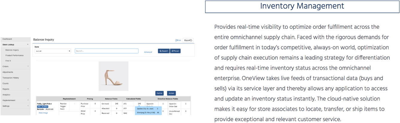
What beyond contractual agreements are needed to coordinate franchise retailers' reordering and sharing decisions? Will some emerging industry practices help? One such practice is the use of disruptive technologies such as the cloud‐based platform developed by OneView (Johnson, 2020). As shown in Figure 1, OneView platform's Inventory Management module (OVIM), designed and operated by the brand manufacturer (the brand), provides real‐time inventory visibility across the entire franchise network. Its more disruptive feature is enabling all franchise retailers to trade frequently with one another and the brand and hence have virtual access to brand inventory (Palanza, 2016).

FIGURE 1

OneView platform: Inventory Management (OVIM).

Can such an internal inventory‐trading platform help coordinate retailers' inventory decisions for a franchise network with multiple inventory‐sharing opportunities? Specifically, are there any coordinating trade rules that the brand is willing to adopt for this platform and all franchise retailers are willing to accept? When developing the trade rules,2 we assume that the brand (he) allows his retailers (she) to make independent inventory‐trading decisions and offers multiple trading opportunities3 during a selling season to best meet consumer demand. The brand should prepare for the possible effect of such trading on his own profit and how to adjust his revenue model. In practice, the typical revenue model is collecting from franchise retailers both royalties (for providing services and license) and profit margins (for selling goods) (KPMG, 2017). The royalty can be fixed or a percentage of the retailer's profit (Simpson, 2018b).

Specifically, we build a multiperiod inventory model for a channel, consisting of a brand and two franchise retailers, with two versions: centralized and decentralized. We also extend the model to consider any number of retailers. In the centralized version, the channel is integrated, and the brand decides in each period how to produce and then distribute or redistribute the channel inventory4 across the retailers. In the decentralized version, the brand is about to adopt the OVIM platform and decides the trade rules, which include the fixed royalty,5 the trade prices, and who pays for shipping. The independent retailers, in turn, simultaneously decide whether to accept the rules, anticipating how they will best trade in each period. Their decision‐making interactions are modeled by a Stackelberg game between the brand (leader) and the retailers (followers) and dynamic multiperiod games between the retailers. If the rules are rejected, the channel operates in the old way.6 If the rules are accepted, in each period, the retailers play a dynamic game to simultaneously decide whether and how to trade (buy or sell and the trade quantity) with one another and the brand. The brand then clears their trade orders (matches the buy and sell orders) and produces/sells when necessary, serving as a market maker.

We solve these games and find that, in equilibrium, the brand would choose to design the trade rules to coordinate the decentralized channel. Our contribution to the literature is both technical and managerial. First, to the best of our knowledge, this work is the first to design a new coordinating scheme (the rules of the internal inventory trading) that can work for business environments with multiple reordering and sharing opportunities. Second, we find that the coordination for such environments requires both an IT platform that enables internal inventory trading, such as the OVIM, and the brand's proactive involvement as the rule and market maker. Third, the key component of the trade rules is the CTPs (coordinating trade prices), which should be carefully designed to remove inventive misalignment, caused by double marginalization and many other factors unique to inventory sharing. The CTPs must depend on the real‐time channel inventory, and they are quite intuitive (constant or market‐clearing7) and can be automated into the platform ex ante. Fourth, the other components of the trade rules are also important. Unlike a typical franchiser profiting from both margins and royalties, the brand should not profit from trades or margins, but only from royalties, albeit fixed or percentage. The shipping cost can be split between the buyer and the seller in any proportion, but it cannot be subsidized by the brand, even partially, as it leads to overtrading.

The existing literature on inventory‐sharing coordination has well explored the base case, which allows only one‐time sharing between retailers and no reordering from the brand. Our work extends it to allow frequent or multiple sharing‐and‐reordering opportunities during the selling season, suitable for more durable goods with quick‐response production available. More importantly, our insights on the coordination for the extended case (as summarized above) differ significantly from those for the base case. First, while contractual agreements are sufficient for coordinating the base case, IT innovations enabling internal inventory trading are needed in addition for the extended case. Second, while who pays for shipping does not affect the channel coordination in the base case, it can destroy the coordination in the extended case. We hope these actionable and new insights could help franchise companies better utilize new technologies, such as the OVIM, and design an ideal internal inventory‐trading mechanism to allow frequent sharing, best meeting demand and maximizing profit.

The rest of the paper is organized as follows. In Section 2, we review the relevant literature. In Section 3, we introduce the general setting of the multiperiod inventory problem for the case with two retailers. We then analyze the centralized version of the problem and derive the channel‐optimal (first best) solutions in Section 4. In Section 5, we introduce the decentralized version of the problem with internal inventory trading enabled by IT platforms such as the OVIM. We then solve the equilibrium for this problem and design the trade prices to coordinate the retailers' trade decisions in Section 6, and craft the coordinating trade rules that the brand will choose to offer in equilibrium in Section 7. We also extend our model in Section 8 to study the general case with multiple retailers. Finally, we conclude the study in Section 9. The numerical study setup is stated in the Appendix, and all the proofs are contained in the Supporting Information.

LITERATURE REVIEW

Recent operations management research has focused on important operations questions that emerge from the advancement and adoption of disruptive technologies (Olsen & Tomlin, 2020). For example, Dong, Shi, et al. (2022) and Song and Zhang (2019) study how 3D‐printing affects manufacturing strategies and spare‐part logistics, respectively. Dong, Jiang, et al. (2022), Babich and Hilary (2020), and Choi et al. (2020) study the influence of Blockchain on various important operations issues. Many works have studied the operational effects of the sharing economy; see a detailed review by Benjaafar and Hu (2020). Different from these works, we focus on whether and how a disruptive platform that enables internal inventory trading can help achieve channel coordination in a franchise network (with independent retailers or dealers and multiple inventory reordering and sharing opportunities).

In terms of modeling, our work is related to inventory sharing between independent retailers. In this literature, separate models are developed to account for two different types of sharing: lateral and preventive; see the detailed reviews by Paterson et al. (2011), Li (2020), and Silbermayr (2020). Lateral sharing (LS) responds to stockouts after all demand is realized at the end of the selling season; shared inventory goes to the out‐of‐stock retailers to fill their unmet demand. By contrast, preventive sharing (PS) responds to inventory imbalance after current demand, but before future demand, is realized; shared inventory goes to the out‐of‐stock or low‐stock retailers to rebalance the channel inventory in the middle of the selling season. As a result, the LS and PS models reflect the same benefit of sharing (quickly meeting the unmet demand) in different ways, and they both assume8 that sharing occurs immediately after the respective demand is realized. More importantly, the existing LS and PS models only allow a single inventory‐sharing opportunity.

Specifically, most of the above‐mentioned works adopt the LS models where the single sharing opportunity occurs at the end of the selling season to quickly fill the unmet demand as much as possible (see, e.g., Anupindi et al., 2001; Dong & Rudi, 2004; Granot & Sošić, 2003; Hanany et al., 2010; Hezarkhani & Kubiak, 2010; Hu et al., 2007; Huang & Sošić, 2010; Rudi et al., 2001; Shao et al., 2011; Sošić, 2006; Yan & Zhao, 2011, 2015, and Zhao et al., 2005). The rest of the works adopt the PS models where the single sharing occurs in the middle of the selling season to not only quickly fill the unmet demand in the first half of the season, but also rebalance the channel inventory to reduce the potential unmet demand in the second half of the season (see, e.g., Comez et al., 2012; Dong et al., 2010; Lee & Whang, 2002; Li et al., 2017; Rong et al., 2010). Different from these works, our paper considers multiple sharing opportunities using a multiperiod PS model.

Our work is closely related to the inventory‐sharing works that design channel coordination schemes. As mentioned above, these schemes only allow a single sharing opportunity, and most of them are designed for LS. The LS coordination schemes assume that the retailers are cooperative in optimal sharing, while the PS coordination schemes do not. However, both LS and PS coordination schemes are designed along two same dimensions. The first dimension is who directs sharing: externally directed (by the supplier or a third party) or self‐directed (negotiated or agreed). The second dimension is what tool is used to coordinate sharing: transshipment prices (TP), profit allocation (PA) rules, or adjustment prices (AP). Specifically, the self‐directed TP is designed by Rudi et al. (2001), Hu et al. (2007), Rong et al. (2010), and Hezarkhani and Kubiak (2010); the supplier‐directed TP is designed by Yan and Zhao (2011); and the third‐party–directed TP is designed by Hanany et al. (2010) and Yan and Zhao (2015). The self‐directed PA is designed by Anupindi et al. (2001), Granot and Sošić (2003), and Huang and Sošić (2010); the supplier‐directed AP is designed by Li et al. (2017).

The general finding is that only some schemes can coordinate, and the externally directed schemes are usually more effective. Note that all these schemes are designed for single sharing and are based on contractual agreements among one supplier and multiple retailers. Unfortunately, due to different misalignment incentives, none of them can be extended to coordinate multiple sharing opportunities. That said, our multiple‐PS model can be considered as an extension of the single‐PS model studied by Li et al. (2017); besides the difference in the number of PS allowed, Li et al. (2017) assume away shipping costs and propose AP for coordination, while we consider shipping costs and propose internal trading for coordination. This paper is the first to study multiple sharing opportunities for noncooperative retailers and propose a new coordinating scheme: supplier‐directed trade rules. Note that internal inventory trading, enabled by IT platforms such as the OVIM, operates differently from contractual agreements. More importantly, its unique feature—automatic cancellation of sell‐orders outstanding—is essential for channel coordination.

Our work is also related to the multiperiod inventory models for a centralized channel with PS, where the channel consists of a supplier and multiple retailers. For the backorder case, Karmarkar (1981) provides a partial description of the optimal policy, and Karmarkar (1987) continues to offer some bounds; Robinson (1990) proves that the base‐stock policy is optimal, without a complete description of the optimal inventory sharing. Recently, Abouee‐Mehrizi et al. (2015) and Li (2020) offer a complete description of the optimal policy for the lost sales case and the backorder case , respectively. By contrast, our paper studies the decentralized version of the multiperiod model for the backorder case and designs internal‐trade rules to achieve coordination. We follow the standard approach that uses the centralized solution from Li (2020) (with some extension) as a benchmark to design coordination. We first model the decentralized problem with internal inventory trading and then design the coordinating trade rules so that the resulting equilibrium decisions match the centralized solution. To the best of our knowledge, our work is the first to coordinate multiperiod inventory reordering and sharing decisions.

MULTIPERIOD INVENTORY PROBLEM

We consider an N‐period inventory problem for a channel consisting of a brand manufacturer, referred as the brand, and two franchise retailers,

$N\ge 2$

. (The general setting with multiple retailers is studied in Section 8.) Each retailer (she) replenishes inventory of a product from the brand (he) or/and the other retailer periodically during the selling season. For example, each period can be a day or a week depending on the product type. We consider two versions of this problem: centralized and decentralized. In the centralized version, introduced in Section 4, inventory decisions are made by the brand for the whole channel. In the decentralized version, introduced in Section 5, inventory decisions are made by the independent retailers for themselves.

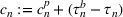
In each period, say period n, there exist production and shipping costs associated with inventory replenishment,

$n=1,\text{…},N$

. The unit cost of production9 borne by the brand is

$c_n^p$

; for simplicity, we assume10 that the production is instantaneous. The unit cost of shipping between the retailers is

${\tau }_n$

, and that between the brand and the retailer is

${\tau }_n^b$

. When the retailers are closer to each other than to the brand, we have

${\tau }_n\le {\tau }_n^b$

, and otherwise, we have

${\tau }_n>{\tau }_n^b$

. For notation brevity, we redenote the unit production cost by

$c_n$

to include the shipping cost difference, that is,

$c_n:=c_n^p+({\tau }_n^b-{\tau }_n)$

; this means that

$(c_n+{\tau }_n)$

is the cost of the channel when a unit is produced by the brand and then shipped to a retailer. Note that to the channel, inventory sharing is only possible (beneficial) if it is cheaper than producing new inventory and then shipping to the retailer (if

${\tau }_n<c_n^p+{\tau }_n^b$

, i.e.,

$c_n>0$

). This assumption seems inevitable, given that our focus is inventory sharing.

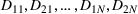
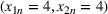
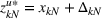
After replenishment at the start of period n, retailer k's inventory is updated from the on‐hand level

$x_{kn}$

to the starting level

$z_{kn}$

, which is used to fill her random demand

$D_{kn}$

. It is important to note that

$z_{kn}$

may be higher or lower than, or the same as,

$x_{kn}$

,

$k=1,2$

. The customer demands,

$D_{11},D_{21},\text{…},D_{1N},D_{2N}$

, can be correlated between retailers and across periods, and any unmet demand is backordered. The sales revenue at

$r_{kn}$

per unit is generated from filling demand immediately with on‐hand inventory and filling backordered demand with urgent delivery from the other retailer or the brand. The channel incurs unit penalty cost

$p_{kn}$

for the backordered demand (to retain the customers). Excess inventory is held through the current period at a unit cost of

$h_{kn}$

for

$n\le N$

; any excess inventory at the end of the selling season (in period N) is salvaged at a unit price v.

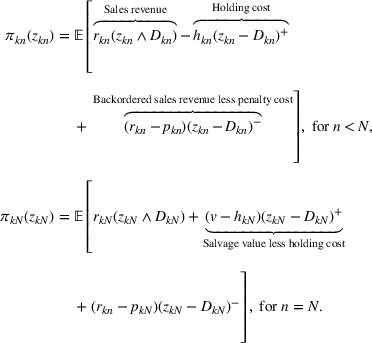
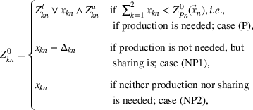
The channel generates revenue from both retailers. Specifically, retailer k's expected revenue

${\pi }_{kn}(z_{kn})$

,

$k=1,2$

, in period n is the sales revenue less the holding and penalty costs, where

1

CENTRALIZED PROBLEM

In the centralized version, the brand serves as the single decision maker. She makes decisions at the start of each period to maximize the channel's profit‐to‐go. These decisions include the production quantity and how to redistribute the channel inventory across the retailers. Note that inventory sharing happens when some inventory of one retailer is redistributed to the other retailer by the brand. We first build a dynamic program for the brand (the channel) and then solve it backward.

At the start of period n, facing the on‐hand channel inventory (

${\vec{x}}_n:=(x_{1n},x_{2n})$

), the brand decides the production quantity (

${\sum }_{k=1}^2{z}_{kn}-{\sum }_{k=1}^2{x}_{kn}\ge 0$

) and then redistributes the channel inventory (

${\sum }_{k=1}^2{z}_{kn}$

) across the retailers so that retailer k will start the period with inventory level

$z_{kn}$

,

$k=1,2$

and

$n\le N$

. This is equivalent to that the brand decides

${\vec{z}}_n:=(z_{1n},z_{2n})$

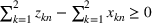
to maximize the channel's profit‐to‐go (in net present value) as follows:

2Recall that

${\pi }_{kn}(z_{kn})$

, defined by (1), is the channel's current‐period revenue earned at retailer k, and

${\mathrm{\Pi }}_{n+1}({\vec{x}}_{n+1})$

is the future profit‐to‐go, which should be discounted by

${\alpha }_n\in [0,1]$

. Maximizing the channel's profit‐to‐go, we obtain the following channel‐optimal solution. Lemma 1

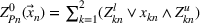
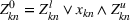
The channel‐optimal solution for period n is to produce‐up‐to

$Z_{Pn}^0({\vec{x}}_n)={\sum }_{k=1}^2(Z_{kn}^l\vee x_{kn}\wedge Z_{kn}^u)$

and redistribute to guarantee that retailer k's starting inventory level is

3where the inventory thresholds

$Z_{1n}^l$

,

$Z_{1n}^u$

,

$Z_{2n}^l$

and

$Z_{2n}^u$

are jointly determined11 by

${\partial }_{z_{kn}}{G}_n({\vec{z}}_n)=c_n+{\tau }_n$

and

${\partial }_{z_{kn}}{G}_n({\vec{z}}_n)=c_n$

,

$k=1,2$

, and for the last period,

$Z_{kN}^l=F_{D_{kN}}^{-1}(\frac{p_{kN}-(c_N+{\tau }_N)}{p_{kN}+h_{kN}-v})$

and

$Z_{kN}^u=F_{D_{kN}}^{-1}(\frac{p_{kN}-c_N}{p_{kN}+h_{kN}-v})$

;

${\vec{\mathrm{\Delta }}}_n:=({\mathrm{\Delta }}_{1n},{\mathrm{\Delta }}_{2n})$

is the optimal shared inventory quantity, which satisfies

${\partial }_{z_{kn}}{G}_n({\vec{x}}_n+{\vec{\mathrm{\Delta }}}_n)-{\tau }_n{1}_{\{{\mathrm{\Delta }}_{kn}>0\}}={\partial }_{z_{-kn}}{G}_n({\vec{x}}_n+{\vec{\mathrm{\Delta }}}_n)-{\tau }_n{1}_{\{{\mathrm{\Delta }}_{-kn}>0\}}$

and

${\mathrm{\Delta }}_{kn}+{\mathrm{\Delta }}_{-kn}=0$

, where “

$-k$

” denotes the other retailer.

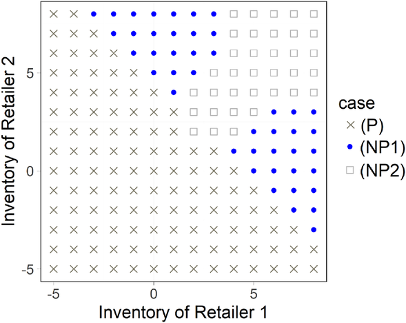
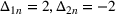
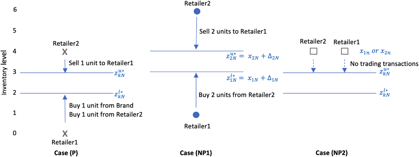
This result extends Li (2020) to allow demand correlation between retailers. It shows that the channel‐optimal solution depends on both the level of the on‐hand channel inventory (

${\sum }_{k=1}^2{x}_{kn}$

) and how it is carried across the two retailers (

$x_{1n},x_{2n}$

), and we may run into case (P), (NP1), or (NP2). This is illustrated by Figure 2, which is based on a simulation12 of two identical retailers with iid Normal demands and has the production threshold as five units. Specifically, case (P) happens when the on‐hand channel inventory (

$x_{1n}+x_{2n}$

) is below the production threshold

$Z_{Pn}^0({\vec{x}}_n)$

; cases (NP1) and (NP2) happen when it is above

$Z_{Pn}^0({\vec{x}}_n)$

. In particular, case (NP1) happens when the on‐hand channel inventory is imbalanced between the retailers (i.e.,

$|x_{1n}-x_{2n}|$

is large enough), while case (NP2) happens when it is balanced (i.e.,

$|x_{1n}-x_{2n}|$

is small enough).

FIGURE 2

Regions of (P), (NP1), and (NP2).

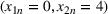
We next explain how the channel‐optimal solution works for each case with the help of Figures 2 and 3. For case (P), the brand should produce‐up‐to the threshold and then allocate the production and arrange necessary sharing between retailers such that every retailer ends up with the optimal level (

$Z_{kn}^0=Z_{kn}^l\vee x_{kn}\wedge Z_{kn}^u$

,

$k=1,2$

). This optimal level is bounded by two thresholds: the lower threshold (

$Z_{kn}^l$

) and the upper threshold (

$Z_{kn}^u$

), as shown in Figure 3. That is, each retailer should receive inventory to raise her level to the lower threshold when her on‐hand is low (

$x_{kn}<Z_{kn}^l$

), share (send‐out) inventory to lower her level to the upper threshold when her on‐hand is high (

$x_{kn}>Z_{kn}^u$

), and do nothing when her on‐hand is medium (

$x_{kn}\in [Z_{kn}^l,Z_{kn}^u]$

). For example, the state/point

$(x_{1n}=0,x_{2n}=4)$

in Figure 2 belongs to case (P), and the corresponding lower and upper thresholds are two and three units, respectively. This means that at this current state (retailer 1 has no inventory and retailer 2 has four units on‐hand), it is channel‐optimal to have retailer 1 receive two units, one from the brand and one from retailer 2, as the arrows indicate in Figure 3.

FIGURE 3

Channel‐optimal solution illustration.

In case (NP1), the channel on‐hand is high enough (and hence no production is needed), but imbalanced between the retailers. To rebalance, it is channel‐optimal to have retailers share

${\vec{\mathrm{\Delta }}}_n$

units of inventory, where

${\mathrm{\Delta }}_{1n}+{\mathrm{\Delta }}_{2n}=0$

. For example, the state

$(x_{1n}=1,x_{2n}=6)$

belongs to this case, and it is channel‐optimal to have retailer 2 share two units with retailer 1 (

${\mathrm{\Delta }}_{1n}=2,{\mathrm{\Delta }}_{2n}=-2$

). This is equivalent to having retailer 2 share two units to lower her inventory to the upper threshold

$x_{2n}+{\mathrm{\Delta }}_{2n}$

and raise retailer 1's inventory to the lower threshold

$x_{1n}+{\mathrm{\Delta }}_{1n}$

, as shown by the arrows in Figure 3. As such sharing reduces the inventory gap between the retailers from five units to one unit, it raises the channel profit the most and hence is considered balanced enough. How small the inventory gap is considered balanced depends on the trade‐off between the cost of sharing (shipping cost) and the benefit of sharing (revenue increase). As the sharing amount (

${\vec{\mathrm{\Delta }}}_n$

) increases, the marginal benefit of sharing (the revenue gain

$|{\partial }_{z_{kn}}{G}_n({\vec{x}}_n+{\vec{\mathrm{\Delta }}}_n)-{\partial }_{z_{-kn}}{G}_n({\vec{x}}_n+{\vec{\mathrm{\Delta }}}_n)|$

) decreases, while the marginal cost (the shipping cost

${\tau }_n$

) remains the same. Therefore, the sharing should stop when the inventory gap is small enough such that the marginal benefit equals the marginal cost. If shipping is more expensive, the channel should have less sharing or tolerate a bigger inventory gap. Note that when shipping is expensive enough, the channel can tolerate a big enough inventory gap so that inventory sharing is never needed, that is, case (NP1) will disappear.

Lastly, in case (NP2), the channel on‐hand inventory is not only high enough, but also balanced between the retailers, and hence even inventory sharing is not needed. For example, as shown in Figure 2, the state

$(x_{1n}=4,x_{2n}=4)$

belongs to this case. It is channel‐optimal to have them remain at the current state (i.e., no inventory redistribution), as illustrated in Figure 3 for this case.

DECENTRALIZED PROBLEM WITH INTERNAL INVENTORY TRADING

In the decentralized version, the retailers are independent decision makers, as in the franchise practice. For simplicity, we assume that before the selling season starts, the retailers have been replenishing inventory from the brand periodically per some supply contracts. Now, the brand attempts to adopt the internal inventory‐trading feature/module in the existing IT platform, such as the OVIM, to connect all the franchise retailers. In this section, we first introduce the sequence of events and the dynamic games and then the decision‐making process of the brand (he) and the retailers (she).

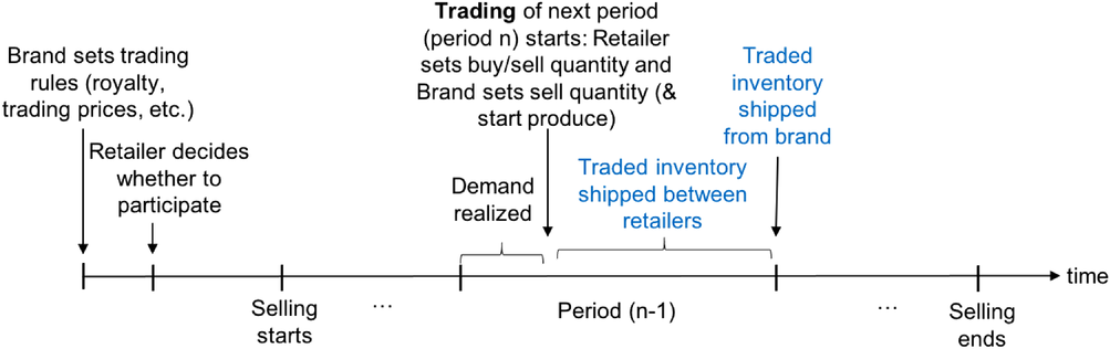
Sequence of events and dynamic games

Before the selling season starts, the brand (leader) and the retailers (followers) play a Stackelberg game on the adoption of the internal inventory trading, and all players are profit maximizers. Specifically, as Figure 4 illustrates, the brand first sets the trade rules, including royalties, trade prices, and who pays for shipping. The retailers, in turn, simultaneously decide whether to participate. If they choose not to participate, the retailers will continue using the supply contracts (they had been using) and earn their reservation profits. If they choose to participate, the retailers will follow the trade rules throughout the selling season.

FIGURE 4

Order of events in the franchise network with inventory trading.

Suppose the retailers choose to participate in the inventory trading. They will then play a multiperiod (or multistage) game and simultaneously decide how to trade (buy or sell and the trade quantity) in every period (stage)13 under information symmetry.14 Although we assume that the inventory trading occurs at the start of period n for presentation simplicity, it can start in period

$(n-1)$

right after both retailers' demands are realized, as illustrated in Figure 4,

$n\le N$

.

During the inventory trading, the retailers submit a buy or sell order of any quantity desired, facing the real‐time trade price and the demand uncertainty of the current and future periods. The brand then clears these orders as the market maker with new production if needed. That is, the traded inventory may come from the other retailer and/or the brand, where the former source may be faster as shown in Figure 4. Any sell orders outstanding, however, will not be executed as the brand never buys back inventory (so that all inventory is held at the retailers to best meet customer demand). Note that such internal inventory trading operates differently from the traditional supply contracts, and we will show that such a difference is essential for coordinating the channels working in the complex environment we study.

Brand's decision: Trade rules

As mentioned above, before the selling season starts, the brand, the leader of the Stackelberg game, decides the trade rules to maximize his own profit. This is equivalent to maximizing the channel profit, as we will prove in Section 7. To reflect the franchise practice, the trade rules include the following three elements:

Royalties: Retailer k pays

${\gamma }_k$

before the selling season,

$k=1,2$

. In practice, it may be paid gradually over time, which will not change our results.

Trade prices: Both retailers can submit a buy or sell order of any quantity at the trade price

$P_{Tn}({\vec{x}}_n)$

15 per unit16 in period n, where

${\vec{x}}_n=(x_{1n},x_{2n})$

is the retailers' on‐hand inventory level,

$n\le N$

.

Shipping: The cost can be split between the buyer and the seller or/and fully or partially covered by the brand.

To maximize his profit, the brand will first match the buy and sell orders as much as possible, achieving inventory sharing between retailers, and then clear any buy‐order outstanding with new production. It is important to compare the internal inventory trading with traditional supply contracts (e.g., wholesale price contracts) from the retailers' perspective. Under the supply contracts, the retailers may not know other retailers' procurement prices, may not have equal prices, and cannot lower their inventory (except via self‐negotiated inventory sharing). By contrast, under the internal inventory trading, the retailers have transparent and equal trade prices, and can lower their inventory (via selling). On the other hand, the supply contracts often offer constant prices, while the internal inventory trading offers market prices, which often depend on supply and demand.

For presentation simplicity, we start by fixing two components of the rules—any given amount of royalties and buyer paying for shipping—and focus on designing the trade prices to coordinate the retailers' inventory decisions. We will then consider the entire trade rules and examine how the brand should optimize them in Section 7.

Retailers' multiperiod games

After the brand (the leader) announces the trade rules, the retailers, as the followers of the Stackelberg game, simultaneously decide whether to participate based on their reservation profits. That is, they will participate if and only if (iff) they expect to earn no less than their reservation profits. If they choose to participate, the retailers will pay their royalties (

${\gamma }_1,{\gamma }_2$

) and then play a multiperiod game, in which they simultaneously decide how to trade in every period. As the royalties are sunk costs and paid upfront, they do not affect the retailers' trading decisions in each period. Therefore, we choose to omit them in the retailers' payoff (profit) functions for each period. The royalties, however, are included when we analyze the retailers' decision on whether to participate in Section 7.

At the start of period n, facing her on‐hand inventory level

$x_{kn}$

(state variable) and random demands of the current and future periods,

$D_{kn},\text{…},D_{kN}$

, retailer k decides her inventory level after trading

$z_{kn}$

(decision variable) simultaneously with the other retailer, retailer

$-k$

, where

$n\le N$

and

$k=1,2$

. Note that deciding

$z_{kn}$

is equivalent to deciding how to trade: buy (

$z_{kn}\ge x_{kn}$

) or sell (

$z_{kn}<x_{kn}$

) at price

$P_{Tn}({\vec{x}}_n)$

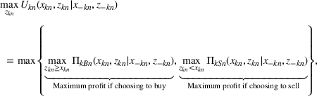
. The retailer k's objective is to maximize her own payoff function

$U_{kn}(x_{kn},z_{kn}|x_{-kn},z_{-kn})$

, representing the expected profit‐to‐go.

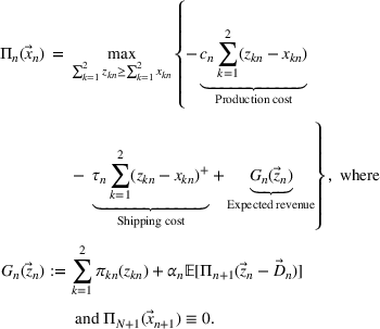
Mathematically, we express retailer k's decision‐making problem as

4where for the trade action

$a=B$

(buy), S (sell), we have

5where

$1_{\{\}}$

is an indicator function,17 the sales profit

${\pi }_{kn}(z_{kn})$

is defined by (1), the future‐period payoff

$U_{k,n+1}^{SPE}(z_{kn}-D_{kn}|z_{-kn}-D_{-kn}):=U_{k,n+1}(z_{kn}-D_{kn},Z_{k,n+1}^{\ast }|z_{-kn}-D_{-kn},Z_{-k,n+1}^{\ast })$

is retailer k's profit‐to‐go of period

$n+1$

under the Subgame‐Perfect Equilibrium (SPE) decisions

$(Z_{1,j}^{\ast },Z_{2,j}^{\ast })$

,

$j\ge n+1$

, and for the last period

$U_{k,N+1}^{SPE}(·|·)\equiv 0$

.

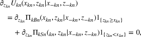
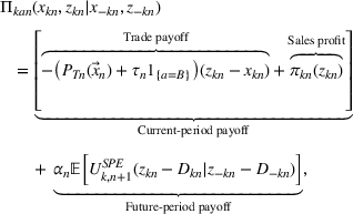
Note that the retailer's payoff function depends on her chosen action, buy or sell, reflected by the shipping cost term (

${\tau }_n{1}_{\{a=B\}}$

); that is, buying comes with the shipping cost, while selling does not.18 Despite her choice of trade, the retailer's payoff function has two parts: one for the current period and one for future periods. Specifically, the current‐period payoff is the trade payoff plus the sales profit. Note that the trade payoff is negative (representing the cost of trading and shipping) when buying, and it is positive (representing the revenue from trading) when selling. The future‐period payoff is the discounted expected profit‐to‐go under the equilibrium. It is important to note that retailer k's future‐period payoff may be affected by the other retailer's decision (

$z_{-kn}$

) through the next period's trade price (

$P_{T,n+1}({\vec{z}}_n-{\vec{D}}_n)$

). That is, in equilibrium, the retailers' decisions will be interdependent for every period, except the last period. As a result, the corresponding inventory‐trading game cannot be reduced to each individual retailer's optimization.

COORDINATING RETAILERS' TRADING DECISIONS

In this section, we consider how to design the trade prices to coordinate the retailers' decisions in each period. That is, we determine the CTPs at which the retailers will trade to start each period with the channel‐optimal inventory level. In other words, these CTPs will induce independent retailers to trade and achieve both the channel‐optimal amount of inventory sharing between the retailers and the channel‐optimal amount of reordering from the brand. Our design of CTPs uses backward induction.

Coordinating the last period (period N)

We start the CTPs' design from the last period. To do so, we first derive the retailers' equilibrium trading decisions for any given trade prices. It is important to note that for generality, we allow for any type of trade prices (

$P_{TN}({\vec{x}}_N)$

), which can be any functions of the state variable (the retailers' on‐hand inventory levels). We then design the CTPs such that the equilibrium trading decisions lead to having the channel‐optimal inventory levels at both retailers.

Equilibrium trading decisions

At the start of period N, facing any given trade price

$P_{TN}({\vec{x}}_N)$

, the retailers simultaneously decide their inventory levels after trading

$(z_{1N},z_{2N})$

to maximize their own payoffs

$(U_{1N},U_{2N})$

, based on their on‐hand inventory levels

$(x_{1N},x_{2N})$

. Their payoffs

$U_{kN}$

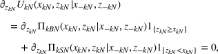
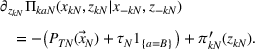
are defined by (4) and (5). To determine the Nash equilibrium (NE), we first derive each retailer's best response, under which her marginal payoff is zero. That is,

6where the marginal payoff depends on the trade action

$a=B$

(buy), S (sell), and

7As shown in (7), the trade action affects the marginal payoff only through the shipping cost term (

${\tau }_N{1}_{\{a=B\}}$

); that is, buying comes with the shipping cost, while selling does not.

Note that retailer k's marginal payoff, and hence her best response, is independent of the other retailer's decision (

$z_{-kN}$

). This means that the retailers' game in the last period can be reduced to individual retailer's optimization. Intuitively, since the selling season ends after period N, retailer k's profit‐to‐go only includes the current‐period profit, which cannot be affected by the other retailer's decision. Therefore, she can completely ignore the other retailer's decision. Solving (6), we obtain each retailer's best response, using which we can then derive the NE as shown below. Note that each retailer's equilibrium trade decision only depends on her own on‐hand inventory level

$x_{kN}$

. Proposition 1

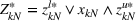
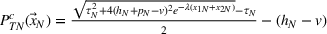
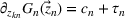
A unique equilibrium (NE) exists, under which retailer k will buy‐up‐to

$z_{kN}^{l\ast }$

(if

$x_{kN}<z_{kN}^{l\ast }$

) or sell‐down‐to

$z_{kN}^{u\ast }$

(if

$x_{kN}>z_{kN}^{u\ast }$

) or do nothing (if

$z_{kN}^{l\ast }\le x_{kN}\le z_{kN}^{u\ast }$

), that is, will trade to maintain inventory level at

$Z_{kN}^{\ast }=z_{kN}^{l\ast }\vee x_{kN}\wedge z_{kN}^{u\ast }$

, where

$z_{kN}^{l\ast }=F_{D_{kN}}^{-1}(\frac{p_{kN}-(P_{TN}({\vec{x}}_N)+{\tau }_N)}{p_{kN}+h_{kN}-v})$

and

$z_{kN}^{u\ast }=F_{D_{kN}}^{-1}(\frac{p_{kN}-P_{TN}({\vec{x}}_N)}{p_{kN}+h_{kN}-v})$

and they both decrease in

$P_{TN}({\vec{x}}_N)$

,

$k=1,2$

.

In the unique equilibrium, each retailer will only trade when her on‐hand inventory (

$x_{kN}$

) is either high (sell) or low (buy), determined by the upper threshold (

$z_{kN}^{u\ast }$

) or the lower threshold (

$z_{kN}^{l\ast }$

), respectively. That is, each retailer will follow a two‐threshold policy: either buy to raise her inventory to the lower threshold, or sell to lower her inventory to the upper threshold, or do nothing, as illustrated in Figure 5. If both retailers want to sell (i.e., no buyers), their orders will not be executed (a common practice in market exchanges). As a result, no trading transactions will actually take place.

FIGURE 5

Nash equilibrium and coordination illustration.

Note that our equilibrium two‐threshold policy differs from those found in the relevant inventory‐sharing literature, which allows a single sharing opportunity only. Specifically, the policy for LS (e.g., Rudi et al., 2001) does not have fixed thresholds and suggests sharing as much as possible to fill any unmet demand. The policy for the PS that does not combine with reordering and is based on constant TP (e.g., Rong et al., 2010) has a similar structure, but our sharing combines with reordering and is based on state‐dependent market prices. The policy for the PS that combines with reordering (e.g., Li et al., 2017) has a single threshold, not two thresholds. These differences are critical as only the two‐threshold policy based on state‐dependent prices best matches the structure of the channel‐optimal solution, observed by comparing Figures 3 and 5. This means that the internal inventory trading we study is essential for the coordination.

In terms of sensitivity, we find that as the trade price

$P_{TN}({\vec{x}}_N)$

increases, both thresholds will reduce, and so will the retailers' equilibrium inventory levels

$(Z_{1N}^{\ast },Z_{2N}^{\ast })$

. Intuitively, as a trade‐price increase reduces the retailers' incentives to buy, but raises their incentives to sell, it makes them want to keep less inventory (after trading). We next examine how to set the trade price right so that in equilibrium, both retailers will trade to maintain inventory at the channel‐optimal levels, benefiting the whole channel. Recall that such trade prices are referred to as the CTPs.

Designing the CTPs

We now design the CTPs to match the resulting equilibrium inventory level

$Z_{kN}^{\ast }$

obtained above, given in Proposition 1, with the channel‐optimal inventory level

$Z_{kN}^0$

, given in Lemma 1,

$k=1,2$

. A quick comparison between the expressions of

$Z_{kN}^{\ast }$

and

$Z_{kN}^0$

reveals that the former is always bounded by two thresholds, while the latter is bounded by two thresholds only in case (P). This means that the CTPs should be set to match these thresholds at least for case (P).

As stated in the proposition below, we prove that for case (P), the inventory levels are matched (

$Z_{kN}^{\ast }=Z_{kN}^0$

) iff both thresholds are matched with those in the channel‐optimal solution (iff

$z_{kN}^{l\ast }=Z_{kN}^l$

and

$z_{kN}^{u\ast }=Z_{kN}^u$

); this implies that the CTP must equal the production cost (

$P_{TN}({\vec{x}}_N)=c_N$

), which removes the double marginalization to incentivize each retailer to “think for” the brand. For case (NP1), the inventory levels are matched (

$Z_{kN}^{\ast }=Z_{kN}^0$

) iff the lower (upper) threshold is matched if it is channel‐optimal for retailer k to receive (share) (iff

$z_{kN}^{l\ast }=x_{kN}+{\mathrm{\Delta }}_{kN}$

if the channel‐optimal shared amount

${\mathrm{\Delta }}_{kN}>0$

and

$z_{kN}^{u\ast }=x_{kN}+{\mathrm{\Delta }}_{kN}$

if

${\mathrm{\Delta }}_{kN}<0$

). This implies that the CTP must equal both retailers' marginal profit under the channel‐optimal solution (

$P_{TN}^c({\vec{x}}_N)={\pi }_{kN}^{\prime }(x_{kN}+{\mathrm{\Delta }}_{kN})-{\tau }_N{1}_{\{{\mathrm{\Delta }}_{kN}>0\}}$

), which works beyond the double marginalization to incentivize each retailer to “think for” the other one. Note that in this case, the unit cost of the channel is the shipping cost; if only used to remove double marginalization, the CTP would have been equal to the shipping cost. For case (NP2), the CTPs should guarantee no trading transactions, which happens iff both retailers choose to sell or do nothing, leveraging on the unique feature in trading that sell‐orders outstanding will not be executed. We prove that one of such CTPs can be the production cost. Proposition 2

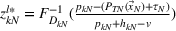
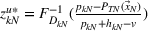
The retailers' last‐period trading decisions are coordinated under the unique equilibrium, when the brand adopts the CTP that satisfies the following in each case:

• (P)

Constant:

$P_{TN}^c({\vec{x}}_N)\equiv c_N$

. (Trading can happen across all parties.)

(NP1)

State dependent:

$P_{TN}^c({\vec{x}}_N)={\pi }_{kN}^{\prime }(x_{kN}+{\mathrm{\Delta }}_{kN})-{\tau }_N{1}_{\{{\mathrm{\Delta }}_{kN}>0\}}$

, together with the lump sum trading reward

$L_{kN}({\vec{x}}_N)$

19. (Trading happens only between retailers.)

(NP2)

Constant:

$P_{TN}^c({\vec{x}}_N)\equiv c_N$

. (No trading happens.)

Recall that the relevant literature, for example, Rong et al. (2010), Yan and Zhao (2015), and Li et al. (2017), has successfully developed various coordinating schemes for the case of a single inventory‐sharing opportunity, and these schemes are all based on contractual agreements. For the business environment with multiple reordering and sharing opportunities (more prevalent in the retail industry), however, contractual agreements do not coordinate even for the last period. Therefore, we examine a new coordinating scheme (internal inventory trading) and characterize the above requirement for one component of this scheme, the trade price. As a result, our findings for the last period are new in several ways. First, the CTP for cases (P) and (NP2) is constant and equal to the production cost, but used for different purposes. For the former (latter) case, the CTP incentivizes retailers to (not to) trade. Thanks to the unique trading feature (cancellation of sell‐orders outstanding), coordination can be attained in case (NP2) via a constant trade price, which is easy to implement. Second, the CTP for case (NP1) should be a two‐party tariff, where the lump sum trading reward is used to completely discourage the retailer's potential strategic trading in the previous period (see a detailed discussion later in this section). Third, the CTP for case (NP1), or specifically the variable part of the CTP, depends on both retailers' on‐hand inventory

${\vec{x}}_N$

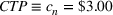
; it is designed to incentivize the retailers to trade only between themselves by the channel‐optimal amount. This CTP generally does not have a closed‐form expression, except for special cases such as exponential demands, and it is lower than the production cost and decreases as any retailer's inventory increases, as shown in Corollary 1 below. Numerically, from Figure 6, we can see that the CTP in case (NP1) is lower than the production cost $3.00; and it can decrease to $2.65, $1.90, and $1.30 as either retailer's inventory goes up. Corollary 1

In case (NP1), the CTP has the following properties:

$P_{TN}^c({\vec{x}}_N)\le c_N$

and decreases in

$x_{1N}$

and

$x_{2N}$

. If the retailers are identical with exponential demand

$(D_{kN}\sim Exp(\lambda ),k=1,2)$

, the CTP has a closed‐form expression:

$P_{TN}^c({\vec{x}}_N)=\frac{\sqrt{{\tau }_N^2+4{(h_N+p_N-v)}^2{e}^{-\lambda (x_{1N}+x_{2N})}}-{\tau }_N}{2}-(h_N-v)$

.

FIGURE 6

Coordinating trade price (CTP; isocurves) of the last period. Note: Two identical retailers with production cost

$c_N=\$3.00$

; simulations with three demand correlations (−0.5, 0, and 0.5) return identical results; lines are isocurves of the variable part of the CTP in case (NP1), and

$CTP\equiv c_n=\$3.00$

in cases (P) and (NP2).

Intuitively, the CTP for cases (P) and (NP1) is the marginal value of inventory when the channel reaches its optimal from the respective current states. That is, it represents the value gained (lost) from having one more (less) unit beyond the channel‐optimal level for the channel or any retailer. When the channel starts from the state in case (P), where inventory is low and production is needed, the marginal value equals the production cost, achieving the optimal (or zero marginal profit). As the channel inventory goes up, it is less valuable to have more inventory, that is, the marginal value drops. Therefore, when the channel starts from the state in case (NP1), where inventory is high and imbalanced and only sharing is needed, the marginal value is less than the production cost, and it is balanced (together with the shipping cost) between the two retailers at optimal sharing. Setting the CTP at this marginal value gives all retailers the right incentives to trade toward the channel‐optimal. Specifically, if a retailer has less (more) inventory than the channel‐optimal, facing such a CTP, it is optimal for her to keep buying (selling) until her marginal inventory value drops (raises) to equal the CTP. As a result, her inventory will be pulled up (down) to match the channel‐optimal, that is, her trading decision is coordinated. For example, as shown in Figure 6, in case (NP1), if the total inventory of the retailers is six units (e.g., in state (1,5) or (5,1)), the CTP is $2.65, which is lower than the production cost ($3.00), and if the total inventory is eight units, the CTP drops to $1.90. By contrast, the CTP for case (NP2), where the channel inventory is high and balanced, is not the marginal value of inventory, but one of the trade prices that can successfully prevent real trading transactions.

The CTP in case (NP1) differs from that in other cases in two ways. First, it is state dependent (not constant) and determined in real time by both retailers' on‐hand inventory levels. It is sort of a market‐clearing price,20 commonly used in economics to represent the equilibrium market price, and therefore it would be intuitive and familiar for all the franchise retailers. Second, it must be a two‐part tariff. The lump sum trading reward is used to prevent strategic trading that roots from the multiperiod trading and the state‐dependent CTPs. That is, the retailers may strategically trade more or less than the channel‐optimal amount in order to manipulate the CTP of the next period. For example, if a retailer anticipates buying (selling) in the next period, she can buy more or sell less (buy less or sell more) now to raise (reduce) her on‐hand inventory in the next period and hence lower (raise) the CTP. With the trading reward, such strategic trading will be completely prevented as it brings them more loss on the reward than the gain on the trade payoff.

As the retailers' demand correlation often affects their joint inventory levels and hence inventory sharing, we next examine its effect on the CTP and have the following results. To the best of our knowledge, the demand correlation has yet to be studied by the relevant literature. Corollary 2

The demand correlation

$Cor(D_{1N},D_{2N})$

does not affect the CTP in the last period.

This result may seem counterintuitive. However, we note that the CTP is derived from the expected channel profit, which in the last period is not affected by the demand correlation. In fact, this profit is the sum of the two retailers' expected sales profits less the production and shipping costs, where only the retailer's sales profit is affected by her own demand distribution, not the demand correlation. For any other period, however, the demand correlation may affect the expected channel profit and hence the CTP.

Coordinating any other period (period

$n<N$

)

Similar to the last period, we design the CTPs to coordinate the retailers' trading decisions in any other period, period

$n<N$

. We do so by backward induction as follows. Suppose that the CTPs are already designed and implemented for all future periods such that both retailers' trading decisions under the unique equilibrium lead to the channel‐optimal inventory levels, that is, such that

$Z_{kj}^{\ast }=Z_{kj}^0$

for all period

$j\ge n+1$

,

$k=1,2$

. Note that this equilibrium is subgame perfect or an SPE, where each subgame is the game starting at each future period. To complete the induction, we first characterize the retailers' equilibrium trading decisions in period n

$(Z_{1n}^{\ast },Z_{2n}^{\ast })$

for any given trade price, and then design the CTP to match them with the channel‐optimal inventory levels

$(Z_{1n}^0,Z_{2n}^0)$

.

Equilibrium trading decisions

At the start of period n, facing any type of given trade price

$P_{Tn}({\vec{x}}_n)$

, the retailers simultaneously decide their inventory levels after trading

$(z_{1n},z_{2n})$

to maximize their own payoffs (profit‐to‐go), based on their on‐hand inventory levels

$(x_{1n},x_{2n})$

. Retailer k's payoff

$U_{kn}$

is defined by (4) and (5),

$k=1,2$

. To determine the equilibrium (SPE), we first derive each retailer's best response, under which her marginal payoff is zero. That is,

8where the marginal payoff depends on the trade action

$a=B$

(buy), S (sell), and

9and

10

Different from the last period, retailer k's marginal payoff, and hence her best response, depends on the other retailer's decision (

$z_{-kn}$

), even if the trade price is constant. This is because her future‐period payoff (

$U_{k,n+1}^{SPE}$

) depends on the CTP of the next period, which is driven by both retailers' decisions (

$z_{kn}$

and

$z_{-kn}$

) or the channel inventory. Such a dependence complicates the analysis, and the best responses must be jointly solved to determine the equilibrium stated below. Proposition 3

A unique equilibrium (SPE) exists, under which in each period n, retailer k will buy‐up‐to

$z_{kn}^{l\ast }(Z_{-kn}^{\ast })$

or sell‐down‐to

$z_{kn}^{u\ast }(Z_{-kn}^{\ast })$

or do nothing, that is, will trade to maintain her inventory at

$Z_{kn}^{\ast }=z_{kn}^{l\ast }(Z_{-kn}^{\ast })\vee x_{kn}\wedge z_{kn}^{u\ast }(Z_{-kn}^{\ast })$

, where the thresholds

$z_{kn}^{l\ast }(z_{-kn})$

and

$z_{kn}^{u\ast }(z_{-kn})$

satisfy

${\partial }_{z_{kn}}{G}_{kn}(z_{kn}|z_{-kn})=P_{Tn}({\vec{x}}_n)+{\tau }_n$

and

${\partial }_{z_{kn}}{G}_{kn}(z_{kn}|z_{-kn})=P_{Tn}({\vec{x}}_n)$

, respectively,

$k=1,2$

.

Note that this result differs from the relevant literature, as we consider internal inventory trading and allow for multiple reordering and sharing opportunities. Comparing to our earlier result for the last period, we find that the equilibrium for every period is a two‐threshold policy, meaning that each retailer will trade (buy or sell) only when her inventory is low or high enough. But, the two thresholds for periods before the last are not constant. Rather, both thresholds of any retailer depend on the other retailer's inventory level. Although we do not have closed‐form expressions for these thresholds, we have the following results on how they are affected by the trade price. Corollary 3

As the trade price

$P_{Tn}({\vec{x}}_n)$

increases, the trading thresholds

$z_{kn}^{l\ast }(z_{-kn})$

and

$z_{kn}^{u\ast }(z_{-kn})$

,

$k=1,2$

, decrease, and so do the equilibrium inventory levels

$(Z_{1n}^{\ast },Z_{2n}^{\ast })$

.

In contrast to the last period, although the two thresholds of the earlier periods are more complex, their dependence on the trade price is similar. That is, as the trade price increases, the two thresholds of both retailers drop, and hence they will buy less or sell more in the equilibrium. This will drive down their inventories and hence the channel inventory. This dependence result helps us design the CTPs.

Designing the CTPs

We now design the CTPs to match the resulting equilibrium inventory level

$Z_{kn}^{\ast }$

, given by Proposition 3, with the channel‐optimal inventory level

$Z_{kn}^0$

, given in Lemma 1,

$k=1,2$

. The comparison between

$Z_{kn}^{\ast }$

and

$Z_{kn}^0$

shows that the former is always bounded by two thresholds, while the latter is bounded by two thresholds only in case (P). This means that the CTPs should be set to match these thresholds at least for case (P).

Unlike in the last period, these thresholds do not have closed‐form expressions and hence cannot be matched directly. The equations they satisfy, however, have a similar format and thus can be matched. Specifically, the thresholds of the equilibrium (

$z_{kn}^{l\ast }(z_{-kn})$

and

$z_{kn}^{u\ast }(z_{-kn})$

) satisfy

${\partial }_{z_{kn}}{G}_{kn}(z_{kn}|z_{-kn})=P_{Tn}({\vec{x}}_n)+{\tau }_n$

and

${\partial }_{z_{kn}}{G}_{kn}(z_{kn}|z_{-kn})=P_{Tn}({\vec{x}}_n)$

, respectively, where

${\partial }_{z_{kn}}{G}_{kn}(z_{kn}|z_{-kn})$

is defined in (10). By contrast, the thresholds of the channel‐optimal solution (

$Z_{kn}^l$

and

$Z_{kn}^u$

) satisfy

${\partial }_{z_{kn}}{G}_n({\vec{z}}_n)=c_n+{\tau }_n$

and

${\partial }_{z_{kn}}{G}_n({\vec{z}}_n)=c_n$

, respectively, where

$G_n({\vec{z}}_n)$

is defined in (2).

To match these equations, we start with their left‐hand sides (

${\partial }_{z_{kn}}{G}_{kn}(z_{kn}|z_{-kn})$

and

${\partial }_{z_{kn}}{G}_n({\vec{z}}_n)$

). Indeed, we find that they are already matched under the CTPs for future periods, that is, we can prove that their difference is zero:

11This is because the trading reward

$L_{k,n+1}({\vec{x}}_{n+1})$

, offered in the next period, can completely neutralize the retailer's incentive of strategic trading. As a result, to achieve coordination, we only need to design

$P_{Tn}({\vec{x}}_n)$

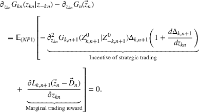
to match the right‐hand sides of these equations for case (P). The trade price design for cases (NP1) and (NP2) requires a similar, but more complex, matching. Overall, our designed CTP for any period is as described below, which is similar to that for the last period. Proposition 4

The retailers' trading decisions in period

$n<N$

are coordinated under the unique SPE, when the brand adopts the CTP that satisfies the following in each case:

• (P)

  Constant:

  $P_{Tn}^c({\vec{x}}_n)\equiv c_n$
  . (Trading happens across all parties.)

• (NP1)

  State dependent:

  $P_{Tn}^c({\vec{x}}_n)={\partial }_{z_{kn}}{G}_{kn}(x_{kn}+{\mathrm{\Delta }}_{kn}|x_{-kn}+{\mathrm{\Delta }}_{-kn})-{\tau }_n{1}_{\{{\mathrm{\Delta }}_{kn}>0\}}$
  , together with the lump sum trading reward
  $L_{kn}({\vec{x}}_n)$
  21. (Trading happens only between retailers.)

• (NP2)

  Constant:

  $P_{Tn}^c({\vec{x}}_n)\equiv c_n$
  . (No trading happens.)

Recall that the existing literature has successfully developed various coordinating schemes for the case of a single inventory‐sharing opportunity, and these schemes are all based on contractual agreements. For the case of multiple reordering and sharing opportunities, our results above show that although the contractual agreements do not coordinate, the internal inventory trading does. Of course, it will require the use of a specific CTP, the CTP, as we characterize. The structure of the CTP for any period remains the same as the last period. As illustrated in Figure 7, the CTP is constant and equals the production cost (

$c_n$

) in cases (P) and (NP2); it is cheaper than the production cost and decreases in the channel inventory in case (NP1), as proved in Corollary 4. Corollary 4

In case (NP1), the CTP has the following properties:

$P_{Tn}^c({\vec{x}}_n)\le c_n$

and decreases in

$x_{1n}$

and

$x_{2n}$

.

FIGURE 7

Coordinating trade price (CTP; isocurves) of period 2. Note: Two identical retailers with production cost

$c_n=\$3.00$

in all four periods

$n=1,\text{…},4$

; lines are isocurves of the variable part of the CTP in case (NP1), and

$CTP\equiv c_n=\$3.00$

in cases (P) and (NP2).

Intuitively, as in the last period, the CTP in case (P) and the variable part of the CTP in case (NP1) represent the value gained (lost) from having one more (less) unit beyond the channel‐optimal level for the channel or any retailer. The CTP in case (NP2), however, is one of the trade prices that can prevent trading transactions from happening. When the channel has more inventory, having one more unit is less valuable. Since the channel has more inventory in case (NP1) than case (P), the marginal value of inventory, or the CTP, is lower, and it is even lower if any player has more inventory.

Different from the last period, both parts of the CTP in case (NP1), the fixed and the variable, depend on not only the retailers' on‐hand inventory levels, but also their future equilibrium inventory levels. Hence, it is a bit complex to calculate and implement, especially facing a large number of periods. For the demand distributions such as exponential, the CTPs may be solved by Mathematica without simulations; for other demand distributions such as Normal, the CTPs have to be searched22 with simulations. The good news is that the brand can have these CTPs all calculated and stored in the trading platform ex ante. As a result, for any state occurred in real time, the corresponding CTP can be shown immediately. These stored CTPs can also be used for the retailers to experience or test, via graphs or/and simulations, before the selling season to facilitate their decisions on whether to accept the trade rules.

We next examine how the CTP is affected by the demand correlation. Analytically, we find23 that, unlike in the last period, the retailers' demand correlation does affect the CTP in other periods. This is because the demand correlation affects the channel profit‐to‐go (which solely determines the CTP) via the joint distribution of retailers' inventory in the next period, and hence the probability of each of the cases (P), (NP1), and (NP2) happening. That is, the demand correlation affects the CTP on the state region of each case, with the additional effect in case (NP1) on the price magnitude.

Numerically, Figure 7 illustrates this effect for period 2 in a four‐period example, where the left, middle, and right panels of the figure correspond to the demand correlation −0.5, 0, and 0.5, respectively. Note that in this example, when the correlation changes from 0 to −0.5, the region of each case remains unchanged, but (the variable part of) the CTP in case (NP1) increases. This means that a negative correlation may raise the trade price, or the marginal value of inventory under the channel‐optimal, when there is pure inventory sharing. When the correlation changes from 0 to 0.5, the region of case (NP1) expands upward and the variable part of the CTP decreases. This means that a positive correlation may increase the chance of pure inventory sharing and also lower the corresponding trade price.

BRAND'S TRADE RULES

We have so far derived the trading prices (CTPs) that the brand should adopt to coordinate the retailers' inventory decisions. In this section, we study how the brand should set the rest of the trade rules to maximize his own profit, which include the royalties and who pays for shipping. Note that the CTP paid to the brand in each period is just enough to cover the production cost; that is, the brand does not profit from coordinating inventory trading. This implies that the brand can only profit from the fixed royalties

$({\gamma }_1,{\gamma }_2)$

collected at the start of the selling season.

As the Stackelberg game leader, the brand can charge any amount of the royalties as long as the retailers are willing to participate, that is, they can earn their reservation profits. Since the royalty is a sunk cost, which does not affect the retailer's trading decisions, the brand can and should charge the highest royalties, leaving the retailers just enough (their reservation profits). This means that the brand earns the channel profit less the retailers' reservation profits. Therefore, in order to maximize his own profit, the brand should aim at maximizing the channel profit. Similar logic has been used in the past literature on channel coordination (Cachon, 2003).

In Section 1, we introduced two types of royalties commonly used in practice. For clarity, our analysis has focused on the fixed type of royalties. Below we prove that all the results also apply to the other type of royalties, a percentage of the retailer's profit. This implies an important actionable guideline to a franchise brand: For his own profit maximization or channel coordination, the type of royalties used does not matter, but the revenue model or source of revenue matters. That is, brands should profit only from the royalties, not from selling goods to the retailers. Proposition 5

In equilibrium, the brand would choose to use the CTPs for trading and charge the fixed royalties

$({\gamma }_1^{\ast },{\gamma }_2^{\ast })$

such that the retailers earn exactly their reservation profits, and the channel coordination is then naturally achieved in all periods. The same results hold true for the other type of royalties used in practice which is a percentage of the retailer's profit.

Regarding the trade rule component that who should pay for shipping, we show that the shipping cost (

${\tau }_n$

) can be split between the buyer and the seller in any proportion. For example, channel coordination is not affected if the buyer and the seller do a 70–30 or 50–50 split of the shipping cost. Interestingly, however, channel coordination collapses if the brand assumes all or even part of the shipping cost, as it leads to overtrading from the retailers (unintended consequences). This result is new to the literature as the relevant past works do not offer any insights on the importance of who pays for shipping cost on channel coordination. Proposition 6

To preserve the channel coordination, the shipping cost (

${\tau }_n$

) can be split between the buyer and the seller in any proportion, but cannot be subsidized by the brand, even partially.

When the shipping cost (

${\tau }_n$

) is split in any proportion, the difference between the buying and selling prices is always

${\tau }_n$

, which is required to achieve the channel coordination where each retailer would buy‐up‐to or sell‐down‐to the respective channel‐optimal thresholds. If the brand assumes all (or part of) the shipping cost, however, the difference between these prices drops to 0 (or below

${\tau }_n$

), and it leads to each retailer buying up‐to or selling down‐to a same threshold (or two closer thresholds), which is overtrading compared with the channel‐optimal solution. This shows that setting up the right trade rules on who pays for shipping is also critical for the channel coordination.

In summary, we have successfully designed a coordinating scheme—the trade rules for the internal inventory trading—to consider environments with multiple reordering and sharing opportunities, which the coordinating schemes in the existing literature cannot accommodate. As the internal inventory trading is explored the first time for its role of channel coordination, we have focused on three basic components of the trade rules: the royalties, the real‐time trade price, and who pays for shipping. Our results show that brands who want to maximize their profits should adopt the coordinating trade rules we characterize, which are likely to differ from what they currently utilize. For example, the royalties must be the only profit source of brands, the trade price must depend on the channel inventory level and can be lower than the production cost, and brands cannot offer any subsidy on shipping.

EXTENSION

We extend our model to study the general case with m ( ≥ 2) retailers. In this case, inventory reallocation (in the centralized version) and inventory trading (in the decentralized version) across retailers become more complex. For example, it is possible that one retailer receives (ships) inventory from (to) many other retailers. Such a complex inventory sharing would be more difficult to achieve in practice without an internal inventory‐trading platform operated by the brand. This means that internal inventory trading is more valuable to brands with a larger franchise network.

Let us compare this general case with the two‐retailer case on modeling, results, and implementation. In terms of modeling, the dynamic games now have more players and are more complex to analyze. However, both the channel's profit‐to‐go

${\mathrm{\Pi }}_n({\vec{x}}_n)$

and each retailer's payoff function

$U_{kn}(x_{kn},z_{kn}|x_{-kn},z_{-kn})$

remain the same as defined in (2) and (4)–(5), respectively. The only difference is that the number of retailers is replaced by m, and

$x_{-kn}$

and

$z_{-kn}$

are now vectors of

$(m-1)$

dimensions. Fortunately, the games can be similarly solved, and the resulting coordinating trade rules24 have a same structure. In terms of implementation, there is additional complexity in both trading transactions and physical shipping due to more players (retailers). As the platform can enable automatic trading transactions, the brand can be freed to focus on facilitating physical shipping only.

CONCLUSIONS

Frequent inventory reallocation, together with quick production, in a franchise network with multiple independent retailers creates a competitive edge, but is challenging to operate and coordinate. This paper examined how to achieve the channel coordination in such a complex environment (with multiple reordering and sharing opportunities). The existing literature has successfully designed various channel coordination schemes for a simpler environment with a single inventory‐sharing opportunity, based on contractual agreements. As these schemes cannot be modified to accommodate multiple such opportunities, this paper designed a new coordination scheme based on the internal inventory trading, enabled by disruptive IT platforms (e.g., the OVIM). Unlike contractual agreements, the internal inventory trading provides a transparent and equal trade price for every retailer.

Analyzing the multiperiod dynamic games among the retailers and the Stackelberg game between the brand and the retailers, we proved that the channel coordination can be naturally achieved in equilibrium. That is, to maximize profit, the brand will implement the coordinating trade rules, and all retailers will accept them. More importantly, we proved that the channel coordination requires both the internal inventory‐trading platform and the brand's proactive involvement as the rule and market maker. The components of the trade rules include the royalties (fixed or percentage), the real‐time CTPs, and who pays for shipping. The coordinating trade rules require the brand to profit only from the royalties and provide no shipping‐cost subsidy. For the royalty, the brand can use any type, fixed or percentage, but must use it as the sole source for profit. That is, unlike in the franchise practice where brands profit from both royalties and margins (from selling goods to retailers), the brand should not profit from inventory trading. Although the shipping cost can be split between the buyer and the seller in any proportion, it cannot be subsidized by the brand, even partially, as any subsidy would lead to overtrading. When serving as the market maker in each period, the brand should respond to the real‐time channel inventory and match the buy and sell orders as much as possible first, and then produce and sell just enough to clear any buy‐orders outstanding.

We characterized the details of the coordinating trade rules. The trade price is the most challenging component to derive as its purpose goes beyond removing the double marginalization. We find that for each period, the CTP is the same regardless of the source of inventory (from the brand or any retailer). The value of the CTPs must depend on the real‐time channel inventory in terms of quantity and distribution across the retailers, in order to align the retailers' incentives with the channel. If the real‐time channel inventory is low (case P) or balanced (case NP2), the CTP should be constant and equal to the production cost; for the former, it is used to simply remove the double marginalization, while for the latter, it is used to induce all retailers to sell and thus prevent any real trade transactions. If the real‐time channel inventory is high and imbalanced (case NP1), the CTP must be a two‐part tariff. The variable part should be state dependent (market‐clearing) and lower than the production cost, and decrease as the channel inventory increases; in this case, trades only happen between the retailers and hence there is no double marginalization, and such a CTP is used to induce all retailers to value their inventories as the channel does. The fixed part of the CTP is a trading reward, which is used to prevent the retailers from strategically holding more or less inventory than the channel‐optimal amount; such a strategic holding aims to manipulate the future trade prices, and it roots from multiperiod trading and state‐dependent trade prices. Moreover, the CTP is affected by the demand correlation across the retailers as the correlation influences how the channel inventory ends up being distributed across retailers in the next period, for example, a more negative (positive) correlation results in a less (more) balanced channel inventory. The good news is that these CTPs are intuitive (constant or market‐clearing) and can be calculated and automated into the internal inventory‐trading platform ex ante.

Our work explored and proved the possibility of coordinating a franchise network in a complex environment (with multiple inventory reordering and sharing opportunities) using a new scheme—the trade rules of internal inventory trading. Our insights highlight the practical importance and necessity of the disruptive IT platforms that enable internal inventory trading, the brand's proactive roles of rule and market maker, the brand's potential behavior change on the revenue model and shipping subsidy, and anticipation of retailers' strategic inventory holding. Our detailed characterization of the coordinating trade rules and actionable insights can guide franchise companies toward best utilizing their channel inventory and improving their profit and customer satisfaction.

APPENDIX: COMPUTATIONAL STUDY

We run a comprehensive numerical study for the cases of two and three retailers with four time periods (

$N=4$

). All franchise retailers and periods are assumed identical. The demand correlations of retailers considered are

$-1,-0.9,\text{…},0.9,1$

. Table A1 describes the base case parameters; deviation from these parameters is also studied.

TABLE A1

Base case parameters.

Retail price	6	Penalty cost	2
Demand	Uniform [0, 5]	Salvage value	2
Production cost	3	Shipping cost	1
Holding cost	0.5	Discount factor	0.9

Note that since the brand only needs to run the computation once for the whole selling season ex ante, the CTPs we characterize are not difficult to implement in practice.