Picking winners: Diversification through portfolio optimization

Abstract

We develop a general framework for selecting a small pool of candidate solutions to maximize the chances that one will be optimal for a combinatorial optimization problem, under a linear and additive random payoff function. We formulate this problem using a two‐stage distributionally robust model, with a mixed 0–1 semidefinite program. This approach allows us to exploit the “diversification” effect inherent in the problem to address how different candidate solutions can be selected to improve the chances that one will attain a high ex post payoff. More interestingly, using this distributionally robust optimization approach, our model recovers the “evil twin” strategy, well known in the field of football pool betting, under appropriate settings.

We also address the computational challenges of scaling up our approach to construct a moderate number of candidate solutions to increase the chances of finding one that performs well. To this end, we develop a sequential optimization approach based on a compact semidefinite programming reformulation of the problem. Extensive numerical results show the superiority of our approach over existing methods.

INTRODUCTION

In the picking winners problem, the goal is to select a portfolio of candidate solutions to maximize the expected “score” of the ex post best‐performing solution (Hunter et al., 2016). The score of each solution is determined by a linear and additive random payoff function, which is based on the solution selected, and the realized payoffs/outcomes in a series of (random) events. This framework can be used to model a variety of problems in “high reward, low probability” winner‐take‐all contests. For example, a venture capital fund selects a set of start‐up companies to invest in, hoping that one of them will achieve huge success in the market. In a similar vein, a contestant in a daily fantasy sports contest chooses multiple lineups (of players) and hopes that one of the lineups selected will obtain a sufficiently high aggregate score to win the contest. Similarly, a contestant enters a sports betting pool with predictions on the outcomes of a series of games, hoping to have the highest number of correct predictions. In all these problems, an ensuing question is to construct a portfolio of candidate solutions so that the ex post performance of the best‐performing candidate is optimal. To this end, we develop a new approach in this paper to capture the “diversification effect” inherent in the portfolio selection problem, overcoming the technical difficulties of performance evaluation using a convex reformulation to approximate the problem.

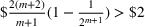
DeStefano et al. (1993) studied a related problem in football pool betting. The goal is to predict the outcome in a series of games (win or lose for the home team), and the punter in the pool with the most number of correct predictions wins the contest. By submitting two entries ($1 for each entry), with the second being the “evil twin” of the first (i.e., bet on the opposite outcome in each game), DeStefano et al. (1993) found that under the independently and identically distributed setting (i.e., outcomes in each game are independent and equally likely), the evil twin strategy can reap significant advantage—when m other punters choose their bets independently in each game with equal probability, the expected return to the evil‐twin strategy is

$\$\frac{2(m+2)}{m+1}(1-\frac{1}{2^{m+1}})>\$2$

. By exploiting the diversification effect in this portfolio with two candidate solutions, the evil twin strategy is able to improve the expected returns from a naive strategy (choosing the outcome in each game randomly).

However, this evil twin strategy does not work well in general situations, especially when the utilities/payoffs for the items are nonidentical and possibly correlated. For the more general case, by assuming that the random payoffs are normally distributed, Hunter et al. (2016) constructed a portfolio guided by a mixed‐integer linear programming model. The goal of this model is to maximize the probability that one of the candidate solutions will win the contest. They used a sequential integer program to construct the portfolio based on the following heuristic: “First, the entries' scores should have a large expected value and variance, which increases the marginal probability of an entry winning. Second, the entries should also have a low correlation with each other to make sure that they cover a large number of possible outcomes.” This inspired the recent work of Bergman et al. (2023), who focused on the construction of two candidate solutions in a portfolio. Under the assumption of normality, they used an associated closed‐form expression of the expected maximum of two (normal) random variables to solve the problem. Based on this result, they designed a branch‐and‐cut algorithm to construct the optimal portfolio in this special case.

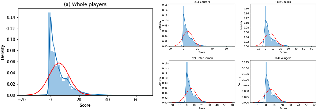
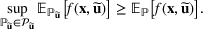
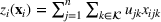
The normality assumption helped simplify the problem and resulted in elegant structural properties. However, extending these insights beyond two candidate solutions appears to be intractable. Furthermore, this assumption may not hold in practice. Take fantasy sports for example. As shown in Figure 1, which plots the fitting probability distributions of the fantasy scores for players using real data. Unfortunately, the best‐fit distribution (colored blue) is clearly different from the normal distribution (colored red).

FIGURE 1

The fitting distribution of the scores for athletes (whole athletes and the athletes under different positions, including center, defensemen, winger, and goalie) using data from October 2, 2019, to January 31, 2021 (https://fantasydata.com/). The blue and red lines correspond to the best‐fit distribution and normal distribution.

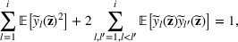
In this study, we use a more direct moment‐based distributionally robust optimization method to construct candidate solutions. This allows us to tap into recent results in the theory of moments by constructing a convex approximation for the problem. More specifically, we use a completely positive cross‐moment model (CPCMM) based on Natarajan et al. (2011). Using this model, we obtain a tight upper bound for the expected value of the stochastic order statistic problem for a given portfolio. Interestingly, this distributionally robust optimization problem can be formulated as a generalized completely positive program (CPP). This approach decomposes the moments matrix (with given means and covariances) into a convex combination of a finite number of rank‐one matrices. This can be viewed as a set of scenarios (with probabilities given by coefficients in the convex combination) that gives rise to the “best‐case” performance of the portfolio. The diversification effect arises because we are constructing a portfolio of solutions that work well in a diverse set of scenarios. This is analogous to Scarf's famous approach to the robust newsvendor solution. By fixing the mean and variance of the demand distribution, Scarf obtained the robust newsvendor solution based on a 2‐point distribution in the worst case (Scarf, 1957). The difference here is that instead of searching for the worst‐case performance (conservative), we solve for the best‐case performance. More importantly, this naturally leads to a tractable mixed 0–1 semidefinite programming (SDP) approximation algorithm, which is used to construct a good portfolio for the picking winners problem.

Notation

We use bold letters to denote the vectors, such as

$\mathbf{x}\in {\mathbb{R}}^n$

, and use bold capital letters to denote the matrices, such as

$\mathbf{A}\in {\mathbb{R}}^{m\times n}$

;

$x_i$

denotes the ith element of vector

$\mathbf{x}$

, and

$A_{ij}$

represents the element in the ith row, jth column of the matrix

$\mathbf{A}$

. We use

${\mathbf{A}}_{i,·}$

(or

${\mathbf{A}}_{·,j}$

) to denote the ith row (or jth column) of the matrix

$\mathbf{A}$

. A random variable or random vector is denoted by a letter with the tilde notation, such as

$\stackrel{\sim }{x}$

and

$\stackrel{\sim }{\mathbf{x}}$

. Specifically, let

$\mathbf{0}$

and

$\mathbf{1}$

denote a vector of all zeros and ones with appropriate size; let

${\mathbf{e}}_i$

represent a vector with one in the ith entry and zeros elsewhere. We use

$\mathbf{O}$

and

$\mathbf{J}$

to denote a matrix of zeros and ones, respectively.

${\mathbf{I}}_n$

denotes an

$n\times n$

identity matrix. Let

${\mathbf{x}}^{\mathrm{T}}$

and

${\mathbf{A}}^{\mathrm{T}}$

denote the transpose of a vector

$\mathbf{x}$

and matrix

$\mathbf{A}$

. We use

$\mathrm{Diag}(\mathbf{x})$

to denote a diagonal matrix with the entries of

$\mathbf{x}$

along the diagonal. Let

$\mathrm{diag}(\mathbf{A})$

represent a vector formed by the diagonal entries of the matrix

$\mathbf{A}$

. The trace of a matrix

$\mathbf{A}$

is denoted by

$\mathrm{Tr}(\mathbf{A})$

. Let

$\mathrm{vec}(\mathbf{A})$

denote the vector obtained by stacking the columns of matrix

$\mathbf{A}$

. Let

$\mathbf{A}•\mathbf{B}$

denote the inner product between matrices

$\mathbf{A}$

and

$\mathbf{B}$

, which is also equivalent to

$\mathrm{Tr}({\mathbf{A}}^{\mathrm{T}}\mathbf{B})$

. We use the notation ○, such as

$\mathbf{A}\circ \mathbf{B}$

and

$\mathbf{x}\circ \mathbf{x}$

, to denote the Hadamard product between two matrices or two vectors. The cardinality of a set is denoted by

$|·|$

. For any integer

$n\in \mathbf{N}$

, [n] is shorthand for set

$\{1,\text{…},n\}$

. We use

$\mathbf{A}{⪰}_{cp}\mathbf{O}$

to represent that

$\mathbf{A}$

is a completely positive matrix and

$\mathbf{A}⪰\mathbf{O}$

to denote that

$\mathbf{A}$

is a positive semidefinite matrix.

LITERATURE REVIEW

Our problem is related to the picking winners problem, sports betting pools, fantasy sports, and SDP‐based approximation methods. We provide a brief review of the literature related to these issues.

The picking winners problem

Our study is inspired by the work of Hunter et al. (2016). They used a greedy heuristic to construct the candidate solutions in a sequential manner, based on the following design principles: maximize the mean and variance of the performance of a solution and minimize the covariance between any two solutions. Hunter et al. (2017) applied this framework to evaluate and choose portfolios of start‐up companies, maximizing the probability that at least one company succeeds. They showed that the objective function in the picking winners problem is submodular and then designed an efficient greedy algorithm to solve the problem. Related applications are discussed in El‐Arini et al. (2009) and Khuller et al. (1999). All the methods proposed thus far exploit properties of normal distribution in the analysis. Our work is different as we relax the assumption of normality for the resources' payoffs and also obtain the diversification effect in the solutions naturally instead of using constraints to enforce this effect.

The problem is also related to the order statistic optimization problem. We refer the interested readers to Ahsanullah and Nevzorov (2005), Bertsimas et al. (2006), and Mehta et al. (2020) for details. More recently, Bergman et al. (2023) focused on the case with two solutions and used results in order statistics (for two normal random variables) to devise cutting plane algorithms for these problems. Our framework is more versatile and can be extended to handle problems with more than two candidate solutions.

Sports betting pools

Kvam and Sokol (2006) and Brown and Sokol (2010) both built linear regression Markov chain models to forecast the outcome of each game in a sports betting pool. Caudill (2003) adopted a maximum score estimator to predict the game outcomes of the NCAA men's basketball tournament. We use these as input in our model to investigate the performance of different sports betting pool strategies. Interestingly, DeStefano et al. (1993) observed that the evil twin strategy has significant advantages when the games in the pool are fair and independent. Kaplan and Garstka (2001) showed how to calculate the mean and variance of the number of accurate guesses for single‐elimination tournaments. They designed a sports betting prediction strategy to maximize the expected total score in an office pool, and they found that the strategy could predict winners in about 58% of games in actual basketball tournaments. Clair and Letscher (2007) developed a new prediction model incorporating pool participant behavior to maximize the expected return in both football pools and tournament‐style pools.

Fantasy sports

A branch of this literature focuses on developing a prediction methodology to estimate player performance based on historical data (see King et al., 2017; Robinson, 2020). Multiple studies have sought to provide an optimization method for sports league drafts. Fry et al. (2007) employed a stochastic program to model the team decision‐making process. Becker and Sun (2016) provided a methodology for predicting athlete and team performance, and they then formulated a mixed 0–1 integer optimization model for draft selection. Readers can refer to Beliën et al. (2017) and Summers et al. (2007) for more details. There are relatively few studies trying to construct portfolios for daily fantasy sports. One notable work is Hunter et al. (2016) mentioned above, which provided a greedy heuristic to construct lineups and achieved great success in actual contests. On this basis, Haugh and Singal (2021) provided an optimization framework to account for an opponent's team selection behavior in daily fantasy sports (DFS). Bergman et al. (2023) also applied their methodology, namely maximizing the expectation of the largest order statistics, to select lineups for DFS.

SDP‐based approximation methods for solving a two‐stage distributionally robust optimization problem

Algorithms for solving a two‐stage distributionally robust optimization problem have been widely studied. Here, we focus specifically on the SDP‐based approximation method, which is closely related to our study. The basic idea of this method is to equivalently reformulate the infinite‐dimensional optimization problem into a finite‐dimensional linear conic program. This method further approximates this cone as a positive semidefinite cone, thus leading to a tractable SDP. For example, G. Xu and Burer (2018) constructed a copositive reformulation to equivalently express the two‐stage robust optimization problem with uncertain right‐hand sides under certain conditions and provided a tractable SDP‐based approximation method to address this problem. Hanasusanto and Kuhn (2018) demonstrated that a two‐stage distributionally robust linear program can be equivalent to a copositive program when the ambiguity set is constructed based on a 2‐Wasserstein ball, leading to a natural SDP approximation. H. Xu et al. (2018) studied a max–max formulation and proved that it can also be equivalent to a copositive program under certain conditions.

Our study focuses on a moment‐based ambiguity set instead of a distance‐based ambiguity set. Applying a moment‐based ambiguity set, Bertsimas et al. (2010) proposed an SDP‐based model for the class of two‐stage minimax distributionally robust linear optimization problems given the first and second moments. Natarajan et al. (2011) proposed a CPCMM to address a two‐stage distributionally robust framework. Their model focuses on a distribution that attains the best‐case expected performance. This model proved that the best‐case expected value of the maximum of a mixed 0–1 linear program was equivalent to a CPP when the decision‐maker knows the first and second moments of the nonnegative uncertain parameters. Since then, the CPCMM model has been applied to many topics (see Gao et al., 2019; Kong et al., 2020; Yan et al., 2018). Note that reformulating into a CPCMM does not immediately make this problem tractable, but it shifts the problem complexity into understanding the facial structure of the completely positive cone or its dual cone (copositive cone). We refer readers to Berman and Shaked‐Monderer (2003) for more information about the two convex cones. One common method is to approximate the completely positive cone as a positive semidefinite cone with nonnegative entries. Therefore, the two‐stage distributionally robust optimization problem can be reduced to a tractable SDP.

We contribute to this literature in two ways. First, we apply the CPCMM to address the portfolio optimization problem in the context of the picking winners problem, which can help naturally exploit the diversification effect via cross‐moments. Second, to overcome the computational inefficiency caused by the high‐dimensional generalized completely positive cone, we collapse the whole optimization problem into a more compact form with a low‐dimensional generalized completely positive cone, thus leading to a tractable mixed 0–1 SDP.

BASIC FRAMEWORK

In this section, we first formally define the picking winners problem and reformulate it into a mixed 0–1 SDP by using a distributionally robust optimization approach. Then we reformulate the basic model using a conic reformulation.

Picking winners: A distributionally robust optimization approach

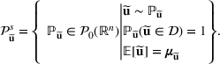
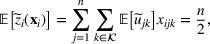
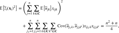
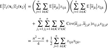
Consider the problem of constructing a portfolio that includes m solutions from n potential resources—the payoff/utilities of which are random and possibly correlated (denoted by

$\stackrel{\sim }{\mathbf{u}}={[{\stackrel{\sim }{u}}_1,\text{…},{\stackrel{\sim }{u}}_n]}^{\mathrm{T}}$

). We denote the ith solution by a binary decision vector

${\mathbf{x}}_i={[x_{i1},\text{…},x_{in}]}^{\mathrm{T}}$

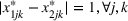
, where

$x_{ij}=1$

if resource j is selected in solution i and 0 otherwise. The payoff is determined by the sum of payoffs of the resources selected, defined as

$${\stackrel{\sim }{z}}_i\left({\mathbf{x}}_i\right)=\sum _{j=1}^n{\stackrel{\sim }{u}}_j{x}_{ij}.$$

Let

$\mathbf{x}=\text{vec}([{\mathbf{x}}_1,\text{…},{\mathbf{x}}_m])\in {\mathbb{R}}^{mn}$

be a binary vector, and let

$\stackrel{\sim }{\mathbf{z}}(\mathbf{x})={[{\stackrel{\sim }{z}}_1({\mathbf{x}}_1),\text{…},{\stackrel{\sim }{z}}_m({\mathbf{x}}_m)]}^{\mathrm{T}}\in {\mathbb{R}}^m$

. The uncertain maximum‐valued solution can be represented as

$$f\left(\mathbf{x},\stackrel{\sim }{\mathbf{u}}\right)=\max \left\{{\stackrel{\sim }{z}}_1\left({\mathbf{x}}_1\right),\text{…},{\stackrel{\sim }{z}}_m\left({\mathbf{x}}_m\right)\right\}.$$

Let

$\stackrel{\sim }{\mathbf{u}}\sim {\mathbb{P}}_{\stackrel{\sim }{\mathbf{u}}}\in {\mathcal{P}}_0({\mathbb{R}}^n)$

. This means that the n‐dimensional random variable,

$\stackrel{\sim }{\mathbf{u}}$

, is governed by a probability distribution

${\mathbb{P}}_{\stackrel{\sim }{\mathbf{u}}}$

, where

${\mathcal{P}}_0({\mathbb{R}}^n)$

represents the set of all probability distributions in

${\mathbb{R}}^n$

. Assume that only the first‐two moments information of

$\stackrel{\sim }{\mathbf{u}}$

is known. Let

${\mathcal{P}}_{\stackrel{\sim }{\mathbf{u}}}$

denote a set of all feasible distributions of

$\stackrel{\sim }{\mathbf{u}}$

supported on

$\mathcal{D}$

with finite mean

${\mathit{\mu }}_{\stackrel{\sim }{\mathbf{u}}}$

and second moment matrix

${\mathrm{\Sigma }}_{\stackrel{\sim }{\mathbf{u}}}$

, that is,

Under this assumption, the picking winners problem of our interest is to optimize the selection decision

$\mathbf{x}$

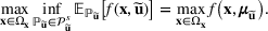
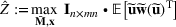
for constructing m solutions so that the best‐case expected performance of the maximum‐valued solution

$f(\mathbf{x},\stackrel{\sim }{\mathbf{u}})$

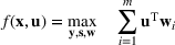
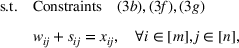
is maximized. The picking winners problem is formulated as follows:

$$Z=\underset{\mathbf{x}\in {\mathrm{\Omega }}_{\mathbf{x}}}{\max }\underset{{\mathbb{P}}_{\stackrel{\sim }{\mathbf{u}}}\in {\mathcal{P}}_{\stackrel{\sim }{\mathbf{u}}}}{sup}{\mathbb{E}}_{{\mathbb{P}}_{\stackrel{\sim }{\mathbf{u}}}}\left[f\left(\mathbf{x},\stackrel{\sim }{\mathbf{u}}\right)\right],$$

1where

${\mathrm{\Omega }}_{\mathbf{x}}$

denotes the feasible region of

$\mathbf{x}$

that can be written in terms of

$\mathbf{x}$

through a set of linear constraints, represented by

$${\mathrm{\Omega }}_{\mathbf{x}}=\left\{\mathbf{x}|\mathbf{A}\mathbf{x}\le \mathbf{b},\mathbf{x}\in {\left\{0,1\right\}}^{mn}\right\}.$$

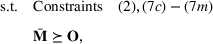
2Note that if we restrict

${\mathbb{P}}_{\stackrel{\sim }{\mathbf{u}}}$

further to contain only the family of normal distributions, and

$\mathcal{D}={\mathbb{R}}^n$

, then

${\mathbb{P}}_{\stackrel{\sim }{\mathbf{u}}}$

is a singleton set. This is because the normal distribution is uniquely determined by the means and covariance conditions. The problem, therefore, reduces to the one studied in the literature. However, with only moments conditions, in general

${\mathcal{P}}_{\stackrel{\sim }{\mathbf{u}}}$

is not a singleton.

For a fixed distribution

${\mathbb{P}}_{\stackrel{\sim }{\mathbf{u}}}$

, there is no closed‐form expression for

${\mathbb{E}}_{{\mathbb{P}}_{\stackrel{\sim }{\mathbf{u}}}}[f(\mathbf{x},\stackrel{\sim }{\mathbf{u}})]$

, which makes the analysis of the picking winners problem intractable. That is, the main challenge of addressing problem (1) lies in its inner problem

${sup}_{{\mathbb{P}}_{\stackrel{\sim }{\mathbf{u}}}\in {\mathcal{P}}_{\stackrel{\sim }{\mathbf{u}}}}{\mathbb{E}}_{{\mathbb{P}}_{\stackrel{\sim }{\mathbf{u}}}}[f(\mathbf{x},\stackrel{\sim }{\mathbf{u}})]$

.

Why max‐sup over max‐inf

Problem (1) is different from the standard robust optimization approach, where the focus is on constructing a “safe” solution that will work well in most scenarios. Instead, the problem in (1) focuses on finding an “optimistic” solution to encourage risk taking and diversification of the solutions constructed. Hence, rather than using an inf formulation to model the second stage performance (as in the traditional robust approach), we use a sup formulation instead. In the following, we show that the inf formulation does not work in this picking winners problem because it does not result in diversification. First, two assumptions are introduced. Assumption 1

The distribution ambiguity set is defined as

Assumption 2

${\mathrm{\Omega }}_{\mathbf{x}}={\mathrm{\Pi }}_{k=1}^m{\mathrm{\Omega }}^{\prime }$

, where

${\mathrm{\Omega }}^{\prime }\subseteq {\{0,1\}}^n$

.

Note that the distribution ambiguity set

${\mathcal{P}}_{\stackrel{\sim }{\mathbf{u}}}^s$

is the same as

${\mathcal{P}}_{\stackrel{\sim }{\mathbf{u}}}$

we study later, except that it relaxes the second moment condition. Assumption 2 ensures that solutions like

$({\mathbf{x}}_0,\text{…},{\mathbf{x}}_0)$

belong to

${\mathrm{\Omega }}_{\mathbf{x}}$

. Theorem 1

Under Assumptions 1 and 2, the max‐inf formulation reduces to

$$\underset{\mathbf{x}\in {\mathrm{\Omega }}_{\mathbf{x}}}{\max }\underset{{\mathbb{P}}_{\stackrel{\sim }{\mathbf{u}}}\in {\mathcal{P}}_{\stackrel{\sim }{\mathbf{u}}}^s}{inf}{\mathbb{E}}_{{\mathbb{P}}_{\stackrel{\sim }{\mathbf{u}}}}\left[f\left(\mathbf{x},\stackrel{\sim }{\mathbf{u}}\right)\right]=\underset{\mathbf{x}\in {\mathrm{\Omega }}_{\mathbf{x}}}{\max }f\left(\mathbf{x},{\mathit{\mu }}_{\stackrel{\sim }{\mathbf{u}}}\right).$$

Furthermore, the optimal portfolio strategy for constructing m solutions satisfies

${\mathbf{x}}^{\ast }=\mathrm{vec}([{\mathbf{x}}_0,\text{…},{\mathbf{x}}_0])$

, where

${\mathbf{x}}_0\in arg{\max }_{{\mathbf{x}}^{\prime }\in {\mathrm{\Omega }}^{\prime }}{\mathit{\mu }}_{\stackrel{\sim }{\mathbf{u}}}•{\mathbf{x}}^{\prime }$

.

Theorem 1 shows that a max‐inf formulation always generates the same m candidate solutions, where any one feasible candidate solution is obtained by maximizing the mean of a portfolio. Therefore, this validates that a max‐inf formulation does not result in diversification. As such, there is no incentive to diversify the portfolio with this model.

On the other hand, the sup formulation has some inherent advantages for this class of problems. For any

${\mathbb{P}}_{\stackrel{\sim }{\mathbf{u}}}\in {\mathcal{P}}_{\stackrel{\sim }{\mathbf{u}}}$

, it is easy to see that

$$\underset{{\mathbb{P}}_{\stackrel{\sim }{\mathbf{u}}}\in {\mathcal{P}}_{\stackrel{\sim }{\mathbf{u}}}}{sup}{\mathbb{E}}_{{\mathbb{P}}_{\stackrel{\sim }{\mathbf{u}}}}\left[f\left(\mathbf{x},\stackrel{\sim }{\mathbf{u}}\right)\right]\ge {\mathbb{E}}_{\mathbb{P}}\left[f\left(\mathbf{x},\stackrel{\sim }{\mathbf{u}}\right)\right].$$

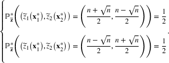
As will be shown later, the left‐hand side can be modeled by a class of conic programs with nice properties—the extremal distribution is obtained from a convex combination of a finite number of outcome “scenarios.” By seeking an “optimistic” solution in this formulation, the diversification effect comes naturally from the risk‐seeking tendency to find a better portfolio. In fact, in the case of sports betting, this model can recover the “evil twin” strategy, where two directly opposing strategies are used to hedge against bad outcomes in a series of sporting contests. For further justifications for using the sup framework, we refer readers to Natarajan et al. (2011) and Natarajan and Teo (2017).

Sports betting pool: Discrete payoffs

In a sports betting pool, each punter places bets based on the outcome of each sporting event in the pool. There are two types of betting pools (Bender, 2013). One is an office pool, where the participants with the maximum number of correct predictions on the outcomes win the entire pool (i.e., a winner‐take‐all payoff structure). The other is a for‐profit pool, where the amount of prize money awarded depends on the number of correct predictions and the payoff structure. In this study, we focus on the office pool version.

Consider n upcoming sports games, in which each game involves two teams (i.e., a home team and an away team). Only one of three outcomes—win, draw, or lose—can occur in each game. Let

$k\in \mathcal{K}=\{-1,0,1\}$

denote the possible outcomes of a game. Specifically, if

$k=-1$

(or 1), the home team loses (wins resp.); otherwise,

$k=0$

indicates a draw. Note that the possible outcomes may only include −1 and 1 in some cases, such as basketball games. In a sports betting pool, punters can submit multiple m

$(m\ge 1)$

entries and the entry with the most correct guesses wins the game.

In the first stage, the punter chooses the outcome of each game, denoted by

${\{{\mathbf{x}}_i\}}_{i=1}^m$

, where

$x_{ijk}=1(j\in [n],k\in \mathcal{K})$

implies that the ith bet of the punter is outcome k in game j. Let

$u_{jk}\in \{0,1\},j\in [n],k\in \mathcal{K}$

, denote the realized outcome, where

$u_{jk}=1$

if the actual result of game j is outcome k and 0 otherwise. Thus, the realized correct guesses of each entry can be depicted as

$z_i({\mathbf{x}}_i)={\sum }_{j=1}^n{\sum }_{k\in \mathcal{K}}{u}_{jk}{x}_{ijk}$

and the corresponding realized correct guesses of the maximum‐valued entry from a punter is

$f(\mathbf{x},\mathbf{u})=\max \{z_1({\mathbf{x}}_1),\text{…},z_m({\mathbf{x}}_m)\}$

.

Reformulation of

$f(\mathbf{x},\mathbf{u})$

Given

$\mathbf{x}$

and realized utilities

$\mathbf{u}$

, the second stage problem aims to select the maximum‐valued solution among m solutions. Let

$y_i=1$

imply that the ith solution is the maximum‐valued solution and 0 otherwise. For linearization purposes, let us introduce the auxiliary variables

$w_{ij}=x_{ij}{y}_i,\forall i\in [m],j\in [n]$

. Then we can equivalently reformulate

$f(\mathbf{x},\mathbf{u})$

as follows:

3a

3b

3c

3d

3e

3f

3g

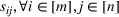
Constraint (3b) assures that only one maximum‐valued solution can be selected. Inequalities (3c)–(3e) are introduced to equivalently express

$w_{ij}=x_{ij}{y}_i$

.

For better computational efficiency (and to ensure tractable formulations later), we further reformulate the above model into a quadratic‐constrained binary program by introducing binary slack variables

$s_{ij},\forall i\in [m],j\in [n]$

. Note that the reformulations that will be developed later will require

$f(\mathbf{x},\mathbf{u})$

to be representable as a quadratic binary program with only equality constraints. By reformulating the linear constraints into a quadratic form, we not only reduce the scale of model constraints in the reformulated conic program but also avoid introducing more slack variables. Specifically, if we solve problem (3) directly, we need to introduce

$3mn$

slack variables (constraints (3c)–(3e) all require

$mn$

slack variables). However, for the quadratic‐constrained binary program below, we only introduce

$mn$

slack variables. Thus, the equivalent quadratic‐constrained binary program is given by

4a

4b

4c

4d

4e We have equivalently transformed the inequality constraints (3c)–(3e) into linear and quadratic constraints (4b)–(4d).

Conic reformulation

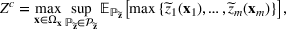
This section aims to reformulate problem (1) into a mixed‐integer conic program with a tractable SDP relaxation. The main challenge of addressing this problem lies in its inner problem:

$$Z_I(\mathbf{x})=\underset{{\mathbb{P}}_{\stackrel{\sim }{\mathbf{u}}}\in {\mathcal{P}}_{\stackrel{\sim }{\mathbf{u}}}}{sup}{\mathbb{E}}_{{\mathbb{P}}_{\stackrel{\sim }{\mathbf{u}}}}\left[f\left(\mathbf{x},\stackrel{\sim }{\mathbf{u}}\right)\right].$$

5The above formulation aims to find a distribution,

${\mathbb{P}}_{\stackrel{\sim }{\mathbf{u}}}$

, for the random variable

$\stackrel{\sim }{\mathbf{u}}$

supported on

$\mathcal{D}$

that satisfies the given first‐two moments (i.e.,

${\mathbb{E}}_{{\mathbb{P}}_{\stackrel{\sim }{\mathbf{u}}}}(\stackrel{\sim }{\mathbf{u}})={\mathit{\mu }}_{\stackrel{\sim }{\mathbf{u}}},{\mathbb{E}}_{{\mathbb{P}}_{\stackrel{\sim }{\mathbf{u}}}}(\stackrel{\sim }{\mathbf{u}}{\stackrel{\sim }{\mathbf{u}}}^{\mathrm{T}})={\mathrm{\Sigma }}_{\stackrel{\sim }{\mathbf{u}}}$

). It must satisfy the corresponding optimal solution,

$(\stackrel{\sim }{\mathbf{y}}(\stackrel{\sim }{\mathbf{u}}),\stackrel{\sim }{\mathbf{w}}(\stackrel{\sim }{\mathbf{u}}),\stackrel{\sim }{\mathbf{s}}(\stackrel{\sim }{\mathbf{u}}))$

, of the quadratic‐constrained binary program,

$f(\mathbf{x},\stackrel{\sim }{\mathbf{u}})$

, so that the term

${\mathbb{E}}_{{\mathbb{P}}_{\stackrel{\sim }{\mathbf{u}}}}[f(\mathbf{x},\stackrel{\sim }{\mathbf{u}})]$

achieves the maximum, or to find a sequence of distributions to asymptotically achieve the maximum. Here, we define

$\stackrel{\sim }{\mathbf{y}}(\stackrel{\sim }{\mathbf{u}})=\mathrm{vec}([{\stackrel{\sim }{y}}_1(\stackrel{\sim }{\mathbf{u}}),\text{…},{\stackrel{\sim }{y}}_m(\stackrel{\sim }{\mathbf{u}})])\in {\mathbb{R}}^m$

,

$\stackrel{\sim }{\mathbf{w}}(\stackrel{\sim }{\mathbf{u}})=\mathrm{vec}([{\stackrel{\sim }{\mathbf{w}}}_1(\stackrel{\sim }{\mathbf{u}}),\text{…},{\stackrel{\sim }{\mathbf{w}}}_m(\stackrel{\sim }{\mathbf{u}})])\in {\mathbb{R}}^{mn}$

, and

$\stackrel{\sim }{\mathbf{s}}(\stackrel{\sim }{\mathbf{u}})=\mathrm{vec}([{\stackrel{\sim }{\mathbf{s}}}_1(\stackrel{\sim }{\mathbf{u}}),\text{…},{\stackrel{\sim }{\mathbf{s}}}_m(\stackrel{\sim }{\mathbf{u}})])\in {\mathbb{R}}^{mn}$

as binary vectors.

In the following, we consider random vector

$\stackrel{\sim }{\mathbf{u}}$

supported on

${\mathbb{R}}^n$

(i.e.,

$\mathcal{D}={\mathbb{R}}^n$

). In this case, it has been established that the inner optimization problem for a set of distributions with prescribed moments is equivalent to a generalized CPP, where the objective function can be written as a linear function of the (conditional) moments and the linear conic constraints are enforced to define the feasible region in the space of moments (Gao et al., 2019; Natarajan et al., 2011; Yan et al., 2018). The advantage of this transformation is that it shifts the difficulty into the convex generalized completely positive cone so that more knowledge about the cone can be applied to multiple types of nondeterministic polynomial time (NP)‐hard problems (Burer, 2009). Specific definitions and properties of the cones of interest, such as generalized completely positive cone and explicit formulations of the CPP, are provided in Appendix EC.1.1 in the Supporting Information.

Define the following rank‐one matrix consisting of the random vector

$\stackrel{\sim }{\mathbf{u}}$

and the corresponding uncertain nonnegative optimal decision vector

$(\stackrel{\sim }{\mathbf{y}}(\stackrel{\sim }{\mathbf{u}}),\stackrel{\sim }{\mathbf{w}}(\stackrel{\sim }{\mathbf{u}}),\stackrel{\sim }{\mathbf{s}}(\stackrel{\sim }{\mathbf{u}}))$

as,

which is a generalized cone of completely positive matrices, that is,

$\stackrel{\sim }{\mathbf{M}}(\stackrel{\sim }{\mathbf{u}},\stackrel{\sim }{\mathbf{y}}(\stackrel{\sim }{\mathbf{u}}),\stackrel{\sim }{\mathbf{w}}(\stackrel{\sim }{\mathbf{u}}),\stackrel{\sim }{\mathbf{s}}(\stackrel{\sim }{\mathbf{u}}))\in \mathcal{C}({\mathbb{R}}^n\times {\mathbb{R}}_{+}^{2mn+m})$

, since

$\stackrel{\sim }{\mathbf{u}}\in {\mathbb{R}}^n$

and

$\stackrel{\sim }{\mathbf{y}}(\stackrel{\sim }{\mathbf{u}}),\stackrel{\sim }{\mathbf{w}}(\stackrel{\sim }{\mathbf{u}}),\stackrel{\sim }{\mathbf{s}}(\stackrel{\sim }{\mathbf{u}})\ge \mathbf{0}$

. We take the expectation of

$\stackrel{\sim }{\mathbf{M}}(\stackrel{\sim }{\mathbf{u}},\stackrel{\sim }{\mathbf{y}}(\stackrel{\sim }{\mathbf{u}}),\stackrel{\sim }{\mathbf{w}}(\stackrel{\sim }{\mathbf{u}}),\stackrel{\sim }{\mathbf{s}}(\stackrel{\sim }{\mathbf{u}}))$

as

6which is used as the decision variable for building the conic program. Note that the decision variable

$\overline{\mathbf{M}}$

still preserves the property of the generalized completely positive cone due to its convexity.

Following the reformulation process of Natarajan et al. (2011), Yan et al. (2018), and Gao et al. (2019), we can get an equivalent generalized CPP for the inner problem (5) of picking winners in terms of decision variable

$\overline{\mathbf{M}}$

, shown in the following problem (7). For the detailed reformulation process, we refer the readers to Appendix EC.1.2 in the Supporting Information.

7a

7b

7c

7d

7e

7f

7g

7h

7i

7j

7k

7l

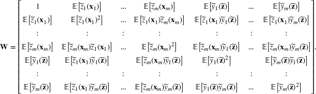
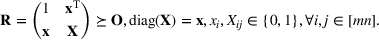
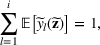
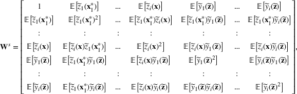
7m where the matrix

${\mathbf{I}}_{n\times mn}=[{\underbrace{{\mathbf{I}}_n,\text{…},{\mathbf{I}}_n}}_m]\in {\mathbf{R}}^{n\times mn}$

. Note that all the expected terms, including

$\mathbb{E}[\stackrel{\sim }{\mathbf{u}}]$

,

$\mathbb{E}[\stackrel{\sim }{\mathbf{y}}(\stackrel{\sim }{\mathbf{u}})]$

,

$\mathbb{E}[\stackrel{\sim }{\mathbf{w}}(\stackrel{\sim }{\mathbf{u}})]$

,

$\mathbb{E}[\stackrel{\sim }{\mathbf{s}}(\stackrel{\sim }{\mathbf{u}})]$

,

$\mathbb{E}[\stackrel{\sim }{\mathbf{u}}{\stackrel{\sim }{\mathbf{u}}}^{\mathrm{T}}]$

,

$\mathbb{E}[\stackrel{\sim }{\mathbf{y}}(\stackrel{\sim }{\mathbf{u}}){\stackrel{\sim }{\mathbf{y}}(\stackrel{\sim }{\mathbf{u}})}^{\mathrm{T}}]$

,

$\mathbb{E}[\stackrel{\sim }{\mathbf{w}}(\stackrel{\sim }{\mathbf{u}}){\stackrel{\sim }{\mathbf{w}}(\stackrel{\sim }{\mathbf{u}})}^{\mathrm{T}}]$

,

$\mathbb{E}[\stackrel{\sim }{\mathbf{w}}(\stackrel{\sim }{\mathbf{u}}){\stackrel{\sim }{\mathbf{s}}(\stackrel{\sim }{\mathbf{u}})}^{\mathrm{T}}]$

,

$\mathbb{E}[\stackrel{\sim }{\mathbf{w}}(\stackrel{\sim }{\mathbf{u}}){\stackrel{\sim }{\mathbf{y}}(\stackrel{\sim }{\mathbf{u}})}^{\mathrm{T}}]$

,

$\mathbb{E}[\stackrel{\sim }{\mathbf{s}}(\stackrel{\sim }{\mathbf{u}}){\stackrel{\sim }{\mathbf{y}}(\stackrel{\sim }{\mathbf{u}})}^{\mathrm{T}}]$

, and

$\mathbb{E}[\stackrel{\sim }{\mathbf{u}}{\stackrel{\sim }{\mathbf{w}}(\stackrel{\sim }{\mathbf{u}})}^{\mathrm{T}}]$

, are the elements of the decision variable

$\overline{\mathbf{M}}$

. Proposition 1

For a given

$\mathbf{x}$

,

$Z_I(\mathbf{x})=Z_{CP}(\mathbf{x})$

.

Proposition 1 indicates the equivalence between problems (5) and (7). Based on Proposition 1, we can directly solve problem (7) instead of solving problem (5), which leads to a convex optimization problem.

However, formulating this problem as a generalized CPP (7) does not resolve the difficulty of the problem. Solving problem (7) is still NP‐hard (Natarajan & Teo, 2017). The difficulty of this problem lies in characterizing the generalized completely positive cone

$\mathcal{C}({\mathbb{R}}^n\times {\mathbb{R}}_{+}^{2mn+m+1})$

(Bomze et al., 2000; Dür & Still, 2008). A simple relaxation method is to approximate the completely positive cone as a “doubly non‐negative cone,” which is defined as a positive semidefinite cone with nonnegative entries, that is,

$\mathbf{A}{⪰}_{cp}\mathbf{O}\approx \mathbf{A}⪰\mathbf{O},\mathbf{A}\ge \mathbf{O}$

. Then by replacing the constraint (7b) with (8b)–(8c) and combining it with the first‐stage optimization problem, the whole picking winners problem (1) can be approximated as a mixed 0–1 SDP program as follows:

8a

8b

8c Clearly, every completely positive cone is doubly nonnegative, but the converse is not necessarily true. Hence, this brings us to the following key result. Proposition 2

Problem (8) provides an upper bound of problem (1), that is,

$Z\le \widehat{Z}$

.

Note that the equation 

$Z=\widehat{Z}$

holds when the dimension of the matrix

$\overline{\mathbf{M}}$

is less than four (Berman & Shaked‐Monderer, 2003). The performance of this relaxation has been shown to work well using simulation (Natarajan et al., 2011). The above framework can also be extended to consider a case with more general support, such as the binary payoff structure in the sports betting pool problem of Subsection 3.1.2. Please refer to Appendix EC.1.3 for more specific details in the Supporting Information.

COMPACT REFORMULATION

In many cases, the number of entries submitted by a punter in a contest is relatively small, compared to the number of resources/players available for selection. For example, there are thousands of start‐up companies every year, but venture capitalists invest in a dozen at most because of cost constraints (Hunter et al., 2017). This motivates us to collapse the above conic program into a more compact form by directly modeling the first and second moment of the payoff of each entry, rather than that of the resources/players.

More specifically, the compact reformulation of interest is defined as follows:

$$Z^c=\underset{\mathbf{x}\in {\mathrm{\Omega }}_{\mathbf{x}}}{\max }\underset{{\mathbb{P}}_{\stackrel{\sim }{\mathbf{z}}}\in {\mathcal{P}}_{\stackrel{\sim }{\mathbf{z}}}}{sup}{\mathbb{E}}_{{\mathbb{P}}_{\stackrel{\sim }{\mathbf{z}}}}\left[\max \left\{{\stackrel{\sim }{z}}_1\left({\mathbf{x}}_1\right),\text{…},{\stackrel{\sim }{z}}_m\left({\mathbf{x}}_m\right)\right\}\right],$$

9where

10Note that in the above compact reformulation, we actually focus on the ambiguity set,

${\mathcal{P}}_{\stackrel{\sim }{\mathbf{z}}}$

, of the utilities of entries

$\stackrel{\sim }{\mathbf{z}}(\mathbf{x})$

rather than

${\mathcal{P}}_{\stackrel{\sim }{\mathbf{u}}}$

of the resources,

$\stackrel{\sim }{\mathbf{u}}$

. To avoid confusion, it is worth emphasizing that, in Section 3, the uncertainty always comes from the distribution of

$\stackrel{\sim }{\mathbf{u}}$

and the distribution of

$\stackrel{\sim }{\mathbf{u}}$

is described by moment‐based ambiguity set

${\mathcal{P}}_{\stackrel{\sim }{\mathbf{u}}}$

. However, the setup of this section is somewhat different. Namely, rather than modeling the distribution of

$\stackrel{\sim }{\mathbf{u}}$

, the goal of this section is to model the distribution of

$\stackrel{\sim }{\mathbf{z}}(\mathbf{x})$

, which is described by the above moment‐based ambiguity set

${\mathcal{P}}_{\stackrel{\sim }{\mathbf{z}}(\mathbf{x})}$

in (10). The following proposition further provides the relationship between the original optimizing problem, (1), and ambiguity set

${\mathcal{P}}_{\stackrel{\sim }{\mathbf{u}}}$

as well as the relationship between compact formulation (9) over ambiguity set

${\mathcal{P}}_{\stackrel{\sim }{\mathbf{z}}(\mathbf{x})}$

. Proposition 3

Problem (9) provides an upper bound to the original problem (1), that is,

$Z^c\ge Z$

.

To better understand the motivation of our compact formulation, we take the following sports betting pool with only two outcomes

$k\in \mathcal{K}=\{-1,1\}$

(i.e., ignoring

$k=0$

) as an example in the next subsection.

Evil twin strategy: Two outcomes per game

The evil twin strategy is to avoid betting on the same outcome in two different entries submitted by the same punter. In this way, one of the entries will always get at least

$n/2$

bets correct. This simple strategy raises the chances that one of the two bets will ultimately win the office pool. DeStefano et al. (1993) verified the significant advantage of the evil twin strategy in their probability model by calculating the associated expected profit of the evil twin strategy. We take this one step further and show that the evil twin strategy is actually the optimal solution in a related distributionally robust optimization model. In the following, we focus on a case of

$m=2$

.

Special case: Equal chance

We consider a special case of the sports betting pool problem that has the following characteristics. For the definition of notations, please refer to Subsection 3.1.2. There are n sport games indexed by

$j\in [n]$

, and each game j has only two different outcomes (i.e.,

$|\mathcal{K}|=2$

): win or lose. Recall that

${\stackrel{\sim }{u}}_{jk}\in \{0,1\},\forall j\in [n],k\in \mathcal{K}$

indicates the uncertain outcomes of each game, where

${\stackrel{\sim }{u}}_{jk}=1$

denotes that the outcome of game j is k and 0 otherwise. We assume that each team has an equal chance of being the winner for each game (i.e.,

${\mathbb{P}}_{\stackrel{\sim }{\mathbf{u}}}({\stackrel{\sim }{u}}_{jk}=1)=\frac{1}{2},\forall j\in [n],k\in \mathcal{K}$

). We also assume that the outcomes in different sports games are independent. In addition, regarding the requirements for betting selection

$\mathbf{x}$

, according to realistic rules for sports betting pools, in each bet, the punter can only bet on exactly one outcome per game (i.e.,

${\mathrm{\Omega }}_{\mathbf{x}}=\{\mathbf{x}\in {\mathbb{R}}^{mn|\mathcal{K}|}|{\sum }_{k\in \mathcal{K}}{x}_{ijk}=1,x_{ijk}\in \{0,1\},\forall i\in [m],j\in [n]\}$

).

Under the above problem settings and based on general compact formulation (9), we can formulate the compact formulation for this special case of the sports betting pool problem. Note that here we actually focus on modeling the joint distribution

${\mathbb{P}}_{\stackrel{\sim }{\mathbf{z}}}$

of the number of correct guesses

$\stackrel{\sim }{\mathbf{z}}(\mathbf{x})={[{\stackrel{\sim }{z}}_1({\mathbf{x}}_1),{\stackrel{\sim }{z}}_2({\mathbf{x}}_2)]}^{\mathrm{T}}$

, where

${\stackrel{\sim }{z}}_i({\mathbf{x}}_i)={\sum }_{j=1}^n{\sum }_{k\in \mathcal{K}}{\stackrel{\sim }{u}}_{jk}{x}_{ijk},\forall i=1,2$

. More precisely, we assume that the distribution

${\mathbb{P}}_{\stackrel{\sim }{\mathbf{z}}}$

of

$\stackrel{\sim }{\mathbf{z}}$

lies in a set of potential joint distributions supported on

${\mathbb{R}}^2$

, with the finite first moment and second moment.

Since

$\stackrel{\sim }{\mathbf{z}}(\mathbf{x})$

is determined by

$\stackrel{\sim }{\mathbf{u}}$

and

$\mathbf{x}$

, the first‐two moment conditions on

$\stackrel{\sim }{\mathbf{z}}(\mathbf{x})$

are also determined by the moments conditions on

$\stackrel{\sim }{\mathbf{u}}$

and the feasible decision

$\mathbf{x}\in {\mathrm{\Omega }}_{\mathbf{x}}$

. Thus, given

$\mathbf{x}$

, the first and second moment of

$\stackrel{\sim }{z_i}({\mathbf{x}}_i)$

,

$\forall i\in \{1,2\}$

, can be expressed as

11a

11b

11cwhere

$\mathrm{Cov}({\stackrel{\sim }{u}}_{j_{1}k},{\stackrel{\sim }{u}}_{j_2{k}^{\prime }}),\forall j_1,j_2\in [n],k,k^{\prime }\in \mathcal{K}$

denotes the covariance between

${\stackrel{\sim }{u}}_{j_{1}k}$

and

${\stackrel{\sim }{u}}_{j_2{k}^{\prime }}$

. For the detailed derivation, we refer the readers to Appendix EC.2.10 in the Supporting Information. We must point out that the independence assumption is not required in Subsection 3.1.2. However, here, the independence assumption for

$\stackrel{\sim }{\mathbf{u}}$

is added to further simplify the first and second moments of

$\stackrel{\sim }{\mathbf{z}}(\mathbf{x})$

. This allows us to derive the evil twin strategy as the optimal solution in this special case.

Therefore, based on the above analysis, in this special case, the compact formulation of the sports betting pool problem can be reduced to the following optimization problem:

$$\underset{\mathbf{x}\in {\mathrm{\Omega }}_{\mathbf{x}}}{\max }\underset{{\mathbb{P}}_{\stackrel{\sim }{\mathbf{z}}}\in {\mathcal{P}}_{\stackrel{\sim }{\mathbf{z}}}}{sup}{\mathbb{E}}_{{\mathbb{P}}_{\stackrel{\sim }{\mathbf{z}}}}\left[\max \left\{{\stackrel{\sim }{z}}_1\left({\mathbf{x}}_1\right),{\stackrel{\sim }{z}}_2\left({\mathbf{x}}_2\right)\right\}\right],$$

12where

13Due to the basic settings of an equal chance of winning and independent outcomes, it is intuitive that the correct guesses for two bets (i.e.,

${\stackrel{\sim }{z}}_1({\mathbf{x}}_1)$

and

${\stackrel{\sim }{z}}_2({\mathbf{x}}_2)$

) will have the same mean and standard deviation. Lemma 1 demonstrates the performance of the evil twin strategy in our moment‐based model. Lemma 1

Optimal betting solution

${\mathbf{x}}^{\ast }$

to problem (12) satisfies

$|x_{1jk}^{\ast }-x_{2jk}^{\ast }|=1,\forall j,k$

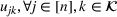
, and the corresponding best‐case expected performance of the maximum‐valued bet equals

$$\underset{{\mathbb{P}}_{\stackrel{\sim }{\mathbf{z}}}\in {\mathcal{P}}_{\stackrel{\sim }{\mathbf{z}}}}{sup}{\mathbb{E}}_{{\mathbb{P}}_{\stackrel{\sim }{\mathbf{z}}}}\left[\max \left\{{\stackrel{\sim }{z}}_1\left({\mathbf{x}}_1^{\ast }\right),{\stackrel{\sim }{z}}_2\left({\mathbf{x}}_2^{\ast }\right)\right\}\right]=\frac{n+\sqrt{n}}{2},$$

which can be exactly achieved by the following extreme two‐point distribution:

$$\left\{\begin{array}{c}\hfill {\mathbb{P}}_{\stackrel{\sim }{\mathbf{z}}}^{\ast }\left(\left({\stackrel{\sim }{z}}_1\left({\mathbf{x}}_1^{\ast }\right),{\stackrel{\sim }{z}}_2\left({\mathbf{x}}_2^{\ast }\right)\right)=\left(\frac{n+\sqrt{n}}{2},\frac{n-\sqrt{n}}{2}\right)\right)=\frac{1}{2}\\ \hfill {\mathbb{P}}_{\stackrel{\sim }{\mathbf{z}}}^{\ast }\left(\left({\stackrel{\sim }{z}}_1\left({\mathbf{x}}_1^{\ast }\right),{\stackrel{\sim }{z}}_2\left({\mathbf{x}}_2^{\ast }\right)\right)=\left(\frac{n-\sqrt{n}}{2},\frac{n+\sqrt{n}}{2}\right)\right)=\frac{1}{2}\end{array}\right..$$

The above result indicates that under this special case, evil twin is the optimal strategy, namely, the optimal solution to problem (12). This affirms the importance of the diversification effect on the performance of the portfolio solution. Even though our moment‐based model is less refined compared to the probability model provided by DeStefano et al. (1993), it still obtains the strategically interesting evil twin strategy as the optimal solution.

General case: Unequal chance

In a more general case, suppose the two outcomes are labeled a and b, that is,

$\mathcal{K}=\{a,b\}$

, with winning probability

$u_{jk},\forall j\in [n],k\in \mathcal{K}$

, for each game j, where

$u_{ja}+u_{jb}=1,\forall j\in [n]$

, and

$u_{ja}>u_{jb}$

. Thus, we have the following optimal betting strategy in this general case. Theorem 2

If each game has two outcomes per game, and the outcomes are independent across games, then the optimal strategy to problem (9) is to sort the games based on

$(2{\mu }_{ja}-1)$

in nonincreasing order:

• ${\mathbf{x}}_1^{\ast }$
  places a bet on the most likely outcome in each game,

• ${\mathbf{x}}_2^{\ast }$
  bets the same as
  ${\mathbf{x}}_1^{\ast }$
  in the first
  $n-l$
  games while then bets against
  ${\mathbf{x}}_1^{\ast }$
  in the last l games, for some
  $l\le n$
  .

Theorem 2 shows that the optimal betting strategy is a “partial” evil twin, balancing between exploitation (for higher winning probabilities) and diversity (evil twin). Note that the complexity of this problem is polynomial‐time

$O(n)$

solvable since we can compute the optimal

$l^{\ast }$

by a simple search in nonincreasing order of

${\mu }_{ja}$

.

Continuous outcomes

It is useful to compare the results obtained above to the continuous outcome case. Suppose that the outcome

${\stackrel{\sim }{u}}_j,\forall j\in [n]$

, of each game is continuous, which follows the standard normal distribution

${\stackrel{\sim }{u}}_j\sim \mathcal{N}(0,1)$

, then the similar problem is defined to solve

${\max }_{\mathbf{x}\in {\mathrm{\Omega }}_{\mathbf{x}}}\mathbb{E}[\max \{{\stackrel{\sim }{z}}_1({\mathbf{x}}_1),{\stackrel{\sim }{z}}_2({\mathbf{x}}_2)\}]$

, where

${\stackrel{\sim }{z}}_i({\mathbf{x}}_i)={\stackrel{\sim }{\mathbf{u}}}^{\mathrm{T}}{\mathbf{x}}_i,i=1,2$

. Assuming

${\mathrm{\Omega }}_{\mathbf{x}}={\{0,1\}}^{2n}$

, Bergman et al. (2023) have shown that this optimization problem is equivalent to

14where

${\sigma }^2({\stackrel{\sim }{z}}_i({\mathbf{x}}_i))$

denotes the variance of the payoff of the ith solution and

$\mathrm{Cov}({\stackrel{\sim }{z}}_1({\mathbf{x}}_1),{\stackrel{\sim }{z}}_2({\mathbf{x}}_2))$

represents the covariance between

${\stackrel{\sim }{z}}_1({\mathbf{x}}_1)$

and

${\stackrel{\sim }{z}}_2({\mathbf{x}}_2)$

. Furthermore, under a special covariance structure, the problem above reduces to a general cut minimization problem (and is therefore NP‐hard!), as the optimal solution satisfies

$x_{1j}^{\ast }+x_{2j}^{\ast }=1$

for all

$j\in [n]$

(Bergman et al., 2023). In the following, we show that our compact formulation can still obtain the same result.

Using the same moment condition as that of Bergman et al. (2023), we set

${\mu }_j=0$

and

${\sigma }_j=1,\forall j\in [n]$

. In this problem setting, similar to problem (12), the compact formulation for the case of continuous outcomes can be described by

$$\underset{\mathbf{x}\in {\mathrm{\Omega }}_{\mathbf{x}}}{\max }\underset{{\mathbb{P}}_{\stackrel{\sim }{\mathbf{z}}}\in {\mathcal{P}}_{\stackrel{\sim }{\mathbf{z}}}}{sup}{\mathbb{E}}_{{\mathbb{P}}_{\stackrel{\sim }{\mathbf{z}}}}\left[\max \left\{{\stackrel{\sim }{z}}_1\left({\mathbf{x}}_1\right),{\stackrel{\sim }{z}}_2\left({\mathbf{x}}_2\right)\right\}\right],$$

15where

16Before analyzing this compact formulation (15), we first give the following important result. Proposition 4

For the problem (15),

$\forall {\mathbb{P}}_{\stackrel{\sim }{\mathbf{z}}}\in {\mathcal{P}}_{\stackrel{\sim }{\mathbf{z}}}$

, given

${\mathbf{x}}_1$

and

${\mathbf{x}}_2$

, we have

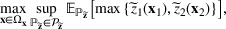
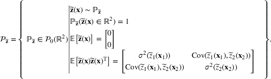
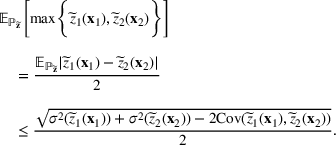
17Moreover, the right‐hand side of inequality (17) is tight since there exists a sequence of random vectors that asymptotically achieves this upper bound, that is,

Proposition 4 indicates that our compact formulation reduces to solving problem (14). Therefore, by referring to Bergman's result mentioned above, the problem of finding the optimal diversification strategy for a portfolio of two or more lineups is NP‐hard in compact reformulation (9), which is formally stated in the following theorem. Theorem 3

Problem (9) is NP‐hard.

This analysis shows that the solution under distributionally robust model (9) is at least as rich as the version considered by Bergman et al. (2023), who used a closed‐form expression for the maximum of two normal random variables to develop a cutting plane algorithm. Our distributionally robust model transforms the problem into a mixed 0–1 SDP, and this allows us to construct a portfolio with three or more lineups, overcoming a key limitation in Bergman et al. (2023). The above also shows a drastic difference in complexity when the outcomes across games change from independent to highly correlated. The latter holds especially for fantasy sports games. We expect that the ability of our model to capture this correlational structure will be extremely valuable for these types of games.

In the case of

$m=2$

, we want to pick two solutions, each with cardinality L (i.e.,

$|{\mathbf{x}}_1|=|{\mathbf{x}}_2|=L$

). Assume that

$n\ge 2L$

. The outcomes are independent and have different means but identical variances. The problem then becomes tractable. The optimal solution follows Theorem 4. Theorem 4

If the outcomes are independent and continuous with different means but the same variance across resources, the optimal strategy for solving Problem (9) is to sort the resources based on

${\mu }_j$

in nonincreasing order:

• ${\mathbf{x}}_1^{\ast }$
  places a bet on L resources with the highest mean outcome,

• ${\mathbf{x}}_2^{\ast }$
  bets the same as
  ${\mathbf{x}}_1^{\ast }$
  in the first
  $L-l$
  resources, while
  ${\mathbf{x}}_2^{\ast }$
  differs from
  ${\mathbf{x}}_1^{\ast }$
  in the last l (
  $l\le L$
  ) resources and bets on the last l resources with the highest mean outcomes outside of those chosen by
  ${\mathbf{x}}_1^{\ast }$
  .

Theorem 4 extends the conclusion in Theorem 2 to the case of continuous payoffs, that partial evil twin is the optimal betting strategy under this special case. Note that the optimal

$l^{\ast }$

can be computed in polynomial‐time

$O(L)$

by a simple line search in nonincreasing order of

${\mu }_j$

.

Furthermore, we consider another special case in which the outcomes for each game have identical mean but have different variances. The optimal betting strategy is formally stated as follows. Corollary 1

Assume

$n\ge 2L$

, If the outcomes are independent and continuous with the same mean and different variance across resources, then the optimal strategy for problem (9) is to sort the resources based on

${\sigma }_j$

in nonincreasing order:

• ${\mathbf{x}}_1^{\ast }$
  bets on L resources, which are randomly selected from the first 2L highest variance outcome and

• ${\mathbf{x}}_2^{\ast }$
  bets on the remaining L resources, which are outside of those chosen by of
  ${\mathbf{x}}_1^{\ast }$
  .

Corollary 1 shows that full evil twin betting on the resources with the highest variances is the best betting strategy in this special case. Recall that the previous evil twin strategies in Theorems 1 and 4 mainly utilize the heterogeneous mean information of each resource (or game) to capture the diversification effect. However, in this case of equal means, the heterogeneous variance is considered to reap the diversification effect.

Reformulation

Note that we have shown the effectiveness of the compact formulation for

$m=2$

in the previous subsection, which can recover the evil twin strategy in both discrete and continuous cases under appropriate settings. In this subsection, we attempt to solve the more general compact formulation (9) for

$m\ge 2$

. To do this, by applying similar techniques in Subsection 3.3, we can further approximate the compact formulation (9) as a low‐dimensional mixed 0–1 SDP.

For a fixed

$\mathbf{x}=\mathrm{vec}([{\mathbf{x}}_1,\text{…},{\mathbf{x}}_m])$

, based on the result of Proposition 1, we can equivalently reformulate the inner problem

$Z_I^c(\mathbf{x})={sup}_{{\mathbb{P}}_{\stackrel{\sim }{\mathbf{z}}}\in {\mathcal{P}}_{\stackrel{\sim }{\mathbf{z}}}}{\mathbb{E}}_{{\mathbb{P}}_{\stackrel{\sim }{\mathbf{z}}}}[\max \{{\stackrel{\sim }{z}}_1({\mathbf{x}}_1),\text{…},{\stackrel{\sim }{z}}_m({\mathbf{x}}_m)\}]$

of problem (9) as a generalized CPP in terms of the decision variable

$\mathbf{W}$

, shown as below:

18a

18b

18c

18d

18e

18f

18gwhere

${\stackrel{\sim }{y}}_i(\stackrel{\sim }{\mathbf{z}})\in \{0,1\},\forall i\in [m]$

is defined as the stochastic optimal decision of problem

$\max \{{\stackrel{\sim }{z}}_1({\mathbf{x}}_1),\text{…},{\stackrel{\sim }{z}}_m({\mathbf{x}}_m)\}$

, and

In the formulation above, similar to problem (7), all the expected terms, including

$\mathbb{E}[{\stackrel{\sim }{z}}_i({\mathbf{x}}_i)],\mathbb{E}[{\stackrel{\sim }{y}}_i(\stackrel{\sim }{\mathbf{z}})],\mathbb{E}[{\stackrel{\sim }{z}}_i({\mathbf{x}}_i){\stackrel{\sim }{z}}_{i^{\prime }}({\mathbf{x}}_{i^{\prime }})],\mathbb{E}[{\stackrel{\sim }{y}}_i{(\stackrel{\sim }{\mathbf{z}})}^2],\mathbb{E}[{\stackrel{\sim }{y}}_i(\stackrel{\sim }{\mathbf{z}}){\stackrel{\sim }{y}}_{i^{\prime }}(\stackrel{\sim }{\mathbf{z}})],\mathbb{E}[{\stackrel{\sim }{z}}_i({\mathbf{x}}_i){\stackrel{\sim }{y}}_i(\stackrel{\sim }{\mathbf{z}})],\forall i,i^{\prime }\in [m]$

, are the elements of the decision variable

$\mathbf{W}$

. Compared with the high‐dimensional

$(2mn+m+n+1)\times (2mn+m+n+1)$

generalized completely positive cone of problem (7), here the inner problem of the compact formulation (18) leads to a low‐dimensional

$(2m+1)\times (2m+1)$

generalized CPP. The corresponding SDP relaxation (i.e.,

$\mathbf{W}\in \mathcal{C}({\mathbb{R}}^m\times {\mathbb{R}}_{+}^{m+1})\approx \mathbf{W}⪰\mathbf{O},{\mathbf{W}}_{[m+2:,m+2:]}\ge \mathbf{O}$

) can now be solved efficiently.

We note that the first stage decisions

$\mathbf{x}\in {\mathrm{\Omega }}_{\mathbf{x}}$

appear in a bilinear form

${\mathbf{x}}_i{\mathbf{x}}_{i^{\prime }}^{\mathrm{T}},\forall i,i^{\prime }(i\ne i^{\prime })\in [m]$

in the above formulation (18). The overall compact formulation (9) is therefore nonconvex in the first stage decision. To speed up the computation further, we convexify the bilinear term based on a semidefinite program. Specifically, the problem is first lifted into a higher dimensional space

by setting

$\mathbf{X}=\mathbf{x}{\mathbf{x}}^{\mathrm{T}}$

and then relaxing the rank‐one constraint by imposing

$\mathbf{X}⪰\mathbf{x}{\mathbf{x}}^{\mathrm{T}}$

. But in our first‐stage problem, in order to obtain binary candidate decision, we retain the binary property of

$\mathbf{x}$

. Thus, the constraint

$\mathbf{X}=\mathbf{x}{\mathbf{x}}^{\mathrm{T}},{\mathbf{x}}_i\in \{0,1\},\forall i\in [mn]$

can be equivalently expressed as follows:

19

Based on the above conic reformulation to the inner problem and the adoption of the convexification technique, we can further approximate the overall compact formulation (9) as the following mixed 0–1 SDP:

20a

20b

20c

20d where the matrix

$\mathbf{X}$

can be partitioned into

$m\times m$

blocks, and

${\mathbf{X}}_{[i{i}^{\prime }]}\in {\mathbb{R}}^{n\times n},\forall i,i^{\prime }\in [m]$

is the

$(i,i^{\prime })$

entry of the original matrix

$\mathbf{X}$

. Proposition 5

Problem (20) provides an upper bound to problem (9), that is,

${\widehat{Z}}^c\ge Z^c$

.

The quality of this compact formulation is examined in Appendix EC.4.1 compared to the original formulation in the Supporting Information.

A sequential optimization algorithm

Although formulation (20) provides a lower dimensional SDP relative to the original formulation (8), it is still computationally costly when we need to construct a large number of entries (i.e., candidate solutions) for the pool. To overcome this issue, we design a sequential optimization algorithm for multiple solutions.

For the first solution, we solve problem (20) by setting

$m=1$

, which is reduced to a 0–1 integer program, that is,

${\max }_{\mathbf{x}\in {\mathrm{\Omega }}_{\mathbf{x}}}{\mathit{\mu }}^{\mathrm{T}}{\mathbf{x}}_1$

.

We calculate the ith (

$2\le i\le m$

) solution

$\mathbf{x}={\mathbf{x}}_i$

based on the first

$i-1$

solutions

${\{{\mathbf{x}}_l^{\ast }\}}_{l=1}^{i-1}$

. By substituting

${\{{\mathbf{x}}_l\}}_{l=1}^{i-1}={\{{\mathbf{x}}_l^{\ast }\}}_{l=1}^{i-1}$

into the problem (20), we obtain the following formulation to obtain

${\mathbf{x}}_i$

. For notational convenience, we use

$\mathbf{x}$

in place of

${\mathbf{x}}_i$

in the rest of the discussion.

21a

21b

21c

21d

21e

21f

21g

21h

21i

21j

21kwhere

and

${\stackrel{\sim }{y}}_l(\stackrel{\sim }{\mathbf{z}})\in \{0,1\},\forall l\in [i]$

, is defined as the optimal solution of the problem

$\max \{{\stackrel{\sim }{z}}_1({\mathbf{x}}_1^{\ast }),\text{…},{\stackrel{\sim }{z}}_i(\mathbf{x})\}$

.

In order to further improve the computational efficiency, we introduce a set of valid inequalities based on a reformulation–linearization technique (RLT) (Sherali & Adams, 2013). Note that an inequality is said to be valid if it is satisfied by all the feasible solutions of problem (21) (Ashraphijuo et al., 2016).

The idea of generating valid inequalities based on RLT is to first generate valid nonconvex quadratic inequalities and then relax them to valid convex inequalities in a lifted space. For example, if

${\mathbf{q}}_1^{\mathrm{T}}\mathbf{x}\ge t_1$

and

${\mathbf{q}}_2^{\mathrm{T}}\mathbf{x}\ge t_2$

are two valid inequalities, then the redundant nonconvex quadratic constraint

$({\mathbf{q}}_1^{\mathrm{T}}\mathbf{x}-t_1)({\mathbf{q}}_2^{\mathrm{T}}\mathbf{x}-t_2)\ge 0$

can be relaxed to the following valid convex inequalities:

which is obtained by relaxing

$\mathbf{X}=\mathbf{x}{\mathbf{x}}^{\mathrm{T}}$

to

$\mathbf{X}⪰\mathbf{x}{\mathbf{x}}^{\mathrm{T}}$

. Similar treatments can be done for the linear constraints on the original decision variable

$\mathbf{x}$

in our problem (21). The difference is that in our case, under the constraint (19),

$\mathbf{X}=\mathbf{x}{\mathbf{x}}^{\mathrm{T}}$

always holds.

• For linear equality constraints

  ${\mathbf{A}}_1\mathbf{x}={\mathbf{b}}_1$
  , a set of lifting equalities are valid, which is given by
  
  22

• For linear inequality constraints

  ${\mathbf{A}}_2\mathbf{x}\le {\mathbf{b}}_2$
  , the redundant nonconvex quadratic constraint
  $({\mathbf{A}}_2\mathbf{x}-{\mathbf{b}}_2){({\mathbf{A}}_2\mathbf{x}-{\mathbf{b}}_2)}^{\mathrm{T}}\ge \mathbf{O}$
  can be relaxed to
  $${\mathbf{A}}_2\mathbf{X}{\mathbf{A}}_2^{\mathrm{T}}-{\mathbf{b}}_2{\mathbf{x}}^{\mathrm{T}}{\mathbf{A}}_2^{\mathrm{T}}-{\mathbf{A}}_2\mathbf{x}{\mathbf{b}}_2^{\mathrm{T}}+{\mathbf{b}}_2{\mathbf{b}}_2^{\mathrm{T}}\ge \mathbf{O}.$$
  23

Thus, the resulting mixed 0–1 SDP formulation for the ith (

$i\ge 2$

) iteration is shown as follows:

24

Comparison between sequential optimization and compact formulation

We use a simple sports betting pool to examine the performance of our sequential optimization method proposed in Section 4.4. We use a dataset of NBA games from November 12, 2020, to November 16, 2020, to obtain the odds for each team, which are used as input for our model. We assume the outcomes of each game are independent to simulate the performance of the solutions obtained. For more details related to the dataset and input estimation, we refer readers to Appendix EC.5.1 in the Supporting Information.

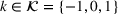
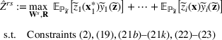
In the test, we vary the number of games (n) from 2 to 6 and the sizes of bets (m) from 1 to 4. Figure 2 reports the results of the objective values and computational times obtained by the two methods (sequential optimization versus compact formulation) under different circumstances. We can observe that the gaps in the objective values obtained by the two methods are quite small, while the computational advantage of our method is significant. Specifically, most of the gaps are within 1%, and the largest gap is 2.82% when

$n=3$

and

$m=4$

. Furthermore, the sequential optimization method obtains the same solution as the compact formulation when

$m=1$

or 2. This is because the sequential optimization method will bet on the most likely outcome in each game in the first iteration, which is one of the optimal solutions when

$m=2$

(as proved in Theorem 2). For the computational time, the sequential optimization method can solve all the scenarios within half a minute, while solving using the compact formulation directly requires an exceedingly long time. For example, it takes more than 36 h to solve

$n=6,m=4$

to optimality. Overall, the sequential optimization method can provide a good approximation for the compact formulation while greatly reducing computational time.

FIGURE 2

Comparisons between sequential optimization and compact formulation. The top and bottom five figures show the results of objective values and computational times, respectively.

Comparison with Hunter's method

To validate the effectiveness of our method, we also compare the performance of sequential optimization in sports betting with a benchmark proposed by Hunter et al. (2016).

Sequential optimization method. We obtain the betting solution

${\{{\mathbf{x}}_i\}}_{i=1}^m$

by applying sequential optimization method (21).

Hunter's method. We apply the framework in Appendix EC.3.2 (in the Supporting Information) to obtain a benchmark solution

${\{{\mathbf{x}}_i^{\mathrm{B}}\}}_{i=1}^m$

.

In the numerical experiments, we assume the outcomes of each game are independent. This is the setting in which heuristics like those in the Hunter method are expected to perform well. Before reporting the results, we first introduce two metrics, the average top‐performing bets and winning probability, to evaluate the out‐of‐sample performance of the solutions obtained. More specifically, we randomly generate

$S=50,000$

runs of the games in the sports betting pool using the outcomes of each game determined by the prescribed odds in the dataset. Each run s is represented by

${\mathbf{u}}_s$

. Based on

${\mathbf{u}}_s$

, we can calculate the top‐performing bet (i.e., the maximum number of correct guesses in the solutions submitted) under the two methods as

$${\widehat{Z}}_s=\underset{i\in [m]}{\max }{\mathbf{u}}_s^{\mathrm{T}}{\mathbf{x}}_i,{\widehat{Z}}_s^{\mathrm{B}}=\underset{i\in [m]}{\max }{\mathbf{u}}_s^{\mathrm{T}}{\mathbf{x}}_i^{\mathrm{B}}.$$

Then, we can compute the two metrics as follows:

• Average top‐performing bets. Let

  $\mathrm{Ave}(\widehat{Z})$
  and
  $\mathrm{Ave}({\widehat{Z}}^{\mathrm{B}})$
  denote the average number of the top‐performing bet for our method and the benchmark, which can be calculated as
  $$\begin{array}{c}\hfill \text{Ave}(\widehat{Z})=\frac{1}{S}\sum _{s=1}^S{\widehat{Z}}_s,\text{Ave}({\widehat{Z}}^{\mathrm{B}})=\frac{1}{S}\sum _{s=1}^S{\widehat{Z}}_s^{\mathrm{B}}.\end{array}$$
  We use
  ${\mathrm{\Delta }}_Z=\mathrm{Ave}(\widehat{Z})-\mathrm{Ave}({\widehat{Z}}^{\mathrm{B}})$
  to measure the improvement of our solution compared to the benchmark.

• Winning probability. We use

  ${\mathrm{P}}_1$
  ,
  ${\mathrm{P}}_2$
  , and
  ${\mathrm{P}}_3$
  to denote the probability that our maximum‐valued bet is equal to, better, and worse than that of benchmark solutions, which is calculated as
  
  We define
  ${\mathrm{\Delta }}_{\mathrm{P}}={\mathrm{P}}_2-{\mathrm{P}}_3$
  to measure the improvement in the winning probability of our top‐performing bet over the benchmark solution. Note that the larger Δ_P, the better our solution is vis‐a‐vis the benchmark.

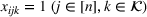
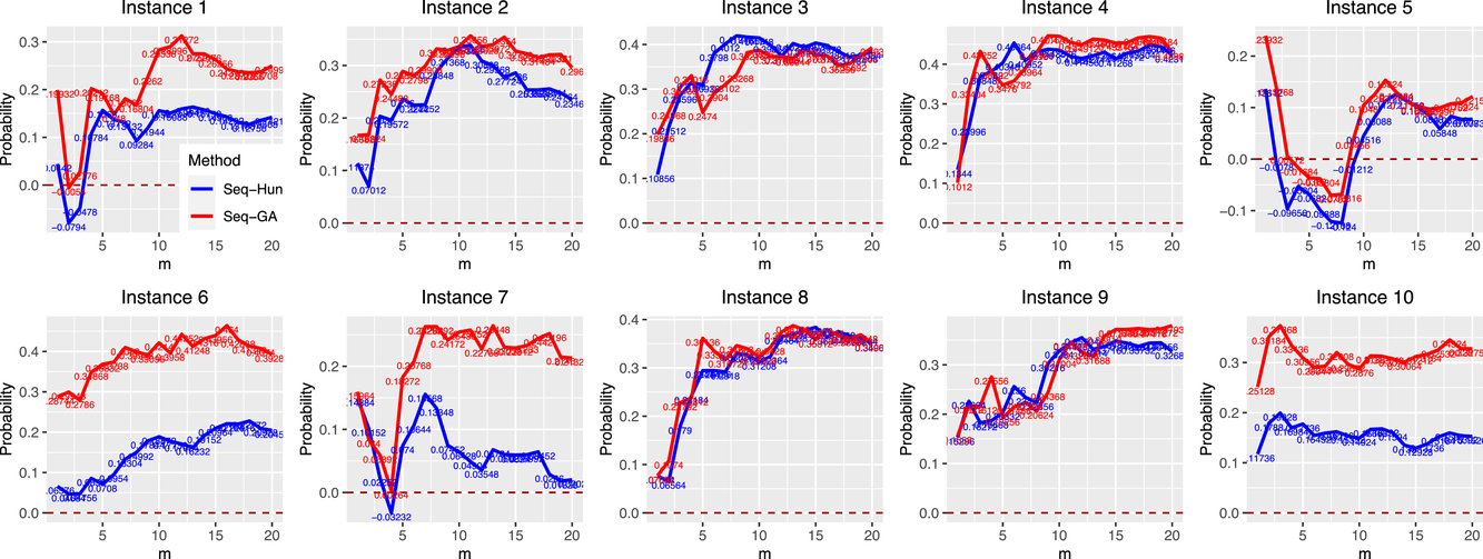
In this test, we vary the number of games (n) from 2 to 7 and the different number of bets (m) from 1 to 8. From Figure 3, we observe that the sequential optimization algorithm performs as well, if not better, than the benchmark in terms of the two metrics. We refer the readers to Appendices EC.5.2 and EC.5.3 (in the Supporting Information) for details on more numerical experiments with this sports betting problem.

FIGURE 3

The results of the comparison between sequential optimization and Hunter's method using NBA games. The top six figures show the average top‐performing bets under the different values of n for the two methods. The bottom two figures report the improvement in the top‐performing bet and the winning probability.

DAILY FANTASY SPORT

In this section, we solve the lineup construction problem for Daily Fantasy Hockey Sports (DraftKings), using data from https://fantasydata.com. We use data from October 2, 2019, to January 31, 2021, as the training set to estimate the parameters for our models. We then use contests from March 1, 2021, to March 10, 2021, as the test set to validate the effectiveness of our method. Specific contest information is shown in Table EC.4 in the Supporting Information.

Problem statement and input estimation

In DraftKings, nearly all winnings go to the top‐performing entry. In the game, each participant can submit multiple hockey lineups (candidate solutions) and the total fantasy score of a lineup is equal to the sum of the real‐world athletes' actual fantasy scores. Each hockey lineup is required to select nine athletes: two centers, three wingers, two defensemen, one goalie, and one utility athlete. Note that the utility athlete can be selected from any of the skaters. Moreover, all the selected athletes of in each hockey lineup must be from at least three different teams, with a budget limit of 50,000 fantasy dollars.

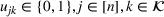
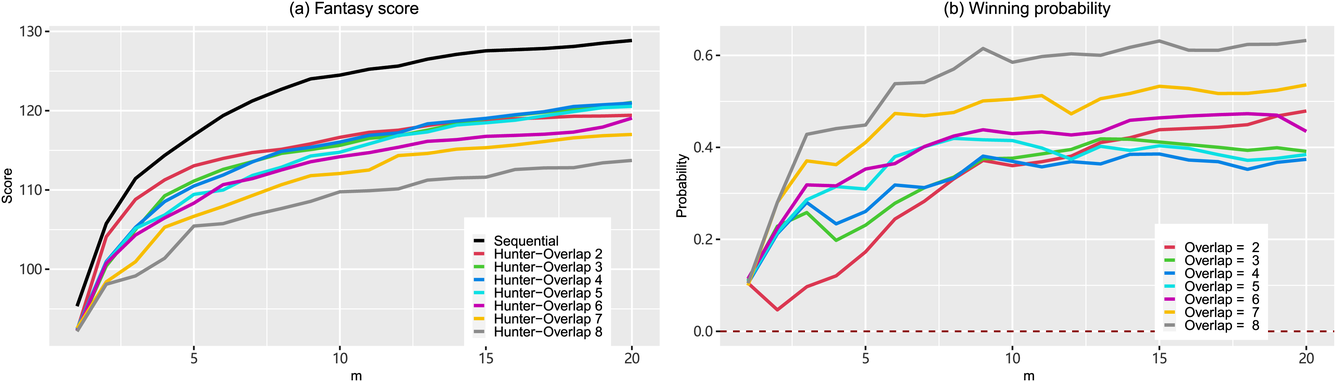
While it is natural to submit as many entries (lineups) as possible in the game, we note that there is a trade‐off between the entry fee and the number of lineups. Hence, it is useful to find a smaller number of lineups with competitive performance. This is particularly relevant, especially for contests with a maximum number of multiple lineup restrictions and high entry fees. As shown in Figure 4, games may restrict the maximum number of lineups. The left one only allows four entries, while the right one allows at most 20 entries. In this case, the ability to generate a moderate number of lineups with high‐quality performance in a reasonable amount of time becomes critical. More examples can be found at https://www.draftkings.com/. For the model formulation and parameters estimations parts, we refer the readers to Appendix EC.6.2 in the Supporting Information.

FIGURE 4

Two examples which set a maximum number of multiple lineup restrictions.

Preprocessing technique

In practice, because there are often hundreds of potential athletes in each contest, it is time‐consuming and not practical to use the sequential optimization method to construct the lineups directly using this universal set of athletes. As shown in Table EC.4 in the Supporting Information, the universal set includes from 123 to 474 athletes for the 10 scenarios we tested. To overcome this problem, we use a simple preprocessing technique to reduce the number of candidate athletes for our method; that is, we simply select the top

$\overline{n}$

athletes based on their projected scores. The reason we do not select players proportionally is that the size of the universal set is different for different contests, which would lead to a huge difference in computation time if we were submitting the same number of lineups in every contest.

Here, we describe how we tune parameter

$\overline{n}$

based on both the solution quality (i.e., objective function) and computational efficiency (i.e., CPU times). In other words, we want to determine an appropriate

$\overline{n}$

that will allow us to generate good solutions with minimal computational time. To do this, we first solve 10 scenarios with

$\overline{n}\in \{30,35,40,45,50,55\}$

to construct a solution with

$m=5$

lineups. Experiments with other choices of m show a similar trend. We use “BNB” in YALMIP to solve the mixed 0–1 SDP. In YALMIP, the gap is defined as

$\frac{UB-LB}{UB+LB}$

, where UB and LB represent the upper and lower bounds in the branch‐and‐bound algorithm. We set the termination gap as 5% to reduce the CPU times in each iteration of the sequential optimization algorithm.

Figure 5a reports the average performance, that is, objective and CPU times, for obtaining five lineups across 10 instances. The objective value increases gradually up till

$\overline{n}=45$

, after which adding more players to the candidate set no longer improves the performance. This is caused by the 5% gap in the termination criterion in each iteration. As shown in Figure 5b, the optimality gaps in each iteration obtained under the case

$\overline{n}=50,55$

are larger than those achieved under the case of

$\overline{n}=45$

or lower. We, therefore, select

$\overline{n}=45$

for the computational experiments performed later. This helps to reduce the computational times, without adversely affecting the solution quality. In practice, as mentioned in Hunter et al. (2017), the goalie information may only be made available about 30 min before games begin, and ideally one should be able to select all the lineups within that time window. This preprocessing technique helps to ensure that our method can generate sufficient lineups within 1800 s. For the detailed results on the 10 instances, we refer the readers to Appendix EC.6.3 in the Supporting Information.

FIGURE 5

Results of preprocessing technique. The left one reports the average objective and total CPU times for five lineups across 10 instances with

$\overline{n}\in \{30,35,40,45,50,55\}$

. The right one shows the optimality gaps in each iteration. CPU, central processing unit.

Comparison with two benchmarks

We compare the performance of our method with two existing benchmarks. The first one is Hunter's method (Hunter et al., 2016) (see Appendix EC.3.3 for more details in the Supporting Information). The second one is a genetic algorithm (GA) proposed by Jarvis Nederlof (see https://levelup.gitconnected.com/dfs‐lineup‐optimizer‐with‐python‐296e822a5309). We solve the solutions for the two benchmarks using all the athletes in the ground set. For our method, we select the 45 athletes with the highest projected scores.

We vary the size of lineups m from 1 to 20 in each scenario. When calculating the out‐of‐sample performance, we assume the true distribution is a multivariate normal distribution,

$\mathcal{N}(\mu ,\mathrm{\Gamma })$

. Note that here the estimated mean of each selected athlete is set as the mean μ of the true distribution. Similarly, the estimated standard deviation of each selected athlete and the estimated correlation matrix together form covariance matrix Γ of the true distribution. Fifty thousand samples are generated to calculate the average score of the top‐performing lineup and winning probability.

Figures 6 and 7, respectively, report the results of the fantasy score comparisons and the improvement in the winning probability. Our method significantly outperforms the other two benchmarks in terms of various metrics. Specifically, our method produces solutions with the highest score among the three methods in all the 10 scenarios tested when

$m=20$

. Interestingly, the improvement in the fantasy score actually increases as the portfolio size increases. This indicates that the advantage of our sequential optimization method becomes more significant as m increases.

FIGURE 6

Results of fantasy score comparisons using daily fantasy hockey contests.

FIGURE 7

Results of winning probability improvement (%) using daily fantasy hockey contests.

To ensure that the outstanding performance of our method originates from the model itself, rather than the selection of the candidate athlete set, we also restrict the ground set for the two benchmarks to the same athlete set as ours (i.e., 45 athletes). Figure 8 plots the fantasy scores obtained by the three methods using 20 lineups. Our method dominates the two benchmarks comprehensively. Note that the Hunter method cannot obtain 20 lineups in some instances because of the hard‐coded overlap constraint used in their approach to diversify the portfolio of solutions. For the detailed results, we refer readers to Appendix EC.6.5 in the Supporting Information.

FIGURE 8

Results of fantasy score comparisons between our method and two benchmarks with

$m=20$

. Here we solve the two benchmarks using the whole athlete set and 45 athletes, respectively.

To show the competitiveness of our model, we also compare our method for

$m=20$

, with the other two benchmarks using more than 20 lineups. That is, we solve the two benchmarks for

$m\in \{20,30,40,50,60,70,80,90,100\}$

lineups. Figure 9 reports the average performance across 10 instances. For the average fantasy score, we observe that our method with 20 lineups can outperform Hunter's method with 50 lineups and is on par with GA with about 70 lineups. Furthermore, our average score is 5.37 points higher than that of Hunter's method with 20 lineups and only 2.60 points smaller than that of Hunter's method with

$m=100$

.

FIGURE 9

Comparisons between our sequential optimization method with

$m=20$

and two benchmarks with

$m\in \{20,30,40,50,60,70,80,90,100\}$

. The left figure reports the average score, and the right one presents the average winning probability improvement (%), that is, Δ_P, across 10 instances.

We observe that the initial set of lineups can be augmented easily with other lineups to deliver superior performance in this problem. To this end, we develop a hybrid algorithm that combines our sequential optimization algorithm and the GA method. Specifically, we generate the first 20 solutions using the sequential optimization algorithm and add the other solutions using the GA proposed by Jarvis Nederlof. In this way, we can obtain many solutions in a reasonable time. We compare this hybrid method with the other two benchmarks with

$m\in \{20,30,40,50,60,70,80,90,100\}$

. Figure 10 reports the average performance across 10 scenarios. We observe that the hybrid algorithm outperforms the other two benchmarks in a comprehensive manner—the initial set of lineups is fundamental to the performance of any algorithm that constructs the full lineups using an incremental method. Our sequential optimization algorithm is particularly useful in this regard. In fact, using an additional 20 lineups constructed using the GA, our hybrid method using 40 lineups can already perform as well as the two benchmarks using 100 lineups.

FIGURE 10

Comparisons between the hybrid algorithm (sequential optimization method + GA) and two benchmarks with

$m\in \{20,30,40,50,60,70,80,90,100\}$

.

Solution structure analysis: Diversification effect

We use the concept of cosine similarity between two bets to measure the diversity effect. This approach is widely used in the machine learning field. Formally, if the candidate set contains n athletes, for any two lineups i and

$i^{\prime }$

, their similarity is defined as,

${\sum }_{i^{\prime }<i}{\sum }_{j=1}^n{x}_{i^{\prime }j}{x}_{ij}$

. Based on this, we can define the diversity of ith lineup in the portfolio as

$1-\frac{{\sum }_{i^{\prime }<i}{\sum }_{j=1}^n{x}_{i^{\prime }j}{x}_{ij}}{9(i-1)}$

, where “9” denotes the total number of athletes selected in each lineup.

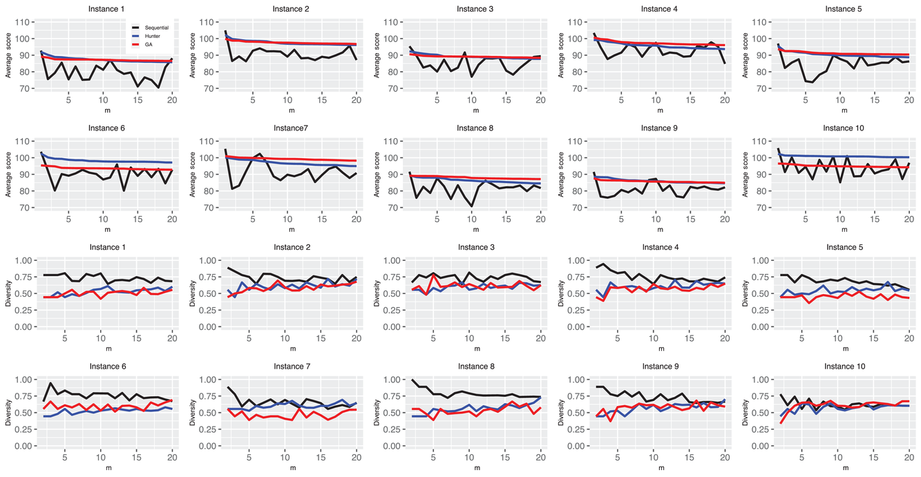
Figure 11 shows the average scores and diversity results for each added lineup. Remarkably, each of our added lineups attains (i) a higher degree of diversity (with the previous lineups) compared with that of the two benchmarks but (ii) each achieves a smaller average fantasy score. This result shows that the existing benchmarks focus more on the marginal score of a lineup for selection, at the expense of diversity, whereas our method focuses more on exploiting the diversification effect, at the expense of individual scores. The former leads to a higher average fantasy score for each added lineup, but the latter has better out‐of‐sample performance for the picking winners problem. In other words, our method improves the portfolio's performance by better exploiting the diversification effect.

FIGURE 11

The results of average scores and diversity for each added lineup. The top 10 graphs report the individual out‐of‐sample performance of each added lineup and the bottom 10 to show the diversity between the lineup added each time and the lineups already in the portfolio.

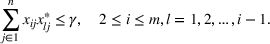
Note that the method in Hunter et al. (2016) handles diversification using a constraint to limit the amount of overlap with previous lineups selected. For current lineup i

$(i\ge 2)$

, and any previous lineup from 1 to

$i-1$

, they add the constraint,

$$\sum _{j\in 1}^n{x}_{ij}{x}_{lj}^{\ast }\le \gamma ,2\le i\le m,l=1,2,\text{…},i-1.$$

25They control the degree of diversification effect by adjusting γ. Next, we vary γ from 2 to 8 in game scenario 3, to investigate how the Hunter method captures the diversification effect. This demonstrates the advantage of our method, in which the diversification effect comes naturally from the model setup. Figure 12 shows the comparison results between our method and the Hunter method with different overlap levels. We can observe that no matter how we control the overlap level, the Hunter method cannot beat our method with the same lineup size.

FIGURE 12

Comparisons between our sequential optimization method and Hunter's method with different overlaps, that is, γ. The left figure reports the average score, and the right one presents the winning probability improvement, that is, Δ_P.

CONCLUDING REMARKS

In this study, we examine portfolio construction under the picking winners framework. Motivated by the good performance of the evil twin strategy in the construction of two‐solution portfolios, we derive a general approach to exploit the diversification effect using a moment‐based two‐stage distributionally robust model. Although this basic framework can be relaxed as a mixed 0–1 SDP, solving an optimal portfolio is still intractable because of the SDP's high dimensionality. To address this issue, we provide a compact reformulation with a lower dimensional SDP. We used these models to “recover” the (partial) evil twin strategy under appropriate settings. To scale up the performance of our approach, we design a sequential optimization method based on the compact formulation. Extensive numerical experiments for sports betting pools and daily fantasy sports using real data demonstrate the superiority of our method compared to the existing benchmarks. The computational results for daily fantasy sports show that our moment‐based model can better exploit the diversification effect compared with other heuristics, thus yielding better out‐of‐sample performance. This implies that adding the diversification effect in building portfolio solutions can help to reduce the risk of uncertainty and thus improve the chances of winning under the framework of the picking winners problem.

The method we propose is not limited to sports betting pools and daily fantasy sports but can be applied to any industry facing a similar portfolio construction problem with a “high reward, low probability” winner‐take‐all structure. Our work can be extended in several directions. One direction is to consider the opponents' behavior when building multiple solutions under the picking winners framework (Haugh & Singal, 2021). This would provide additional insights into the portfolio construction problem and help in building better solutions. Furthermore, the techniques developed in this study can contribute to other related fields, such as product line (Bertsimas & Mišić, 2017) and bundle design (Li et al., 2022). Specifically, the sequential optimization framework based on a low‐dimensional mixed 0–1 SDP can also be applied to the design of product lines or product bundles under appropriate problem settings. We leave these extensions for future research.