Capacity planning with limited information

Abstract

Limited information about the demand for some of the resources needed to produce goods and services (e.g., incomplete and imperfect bills of materials) forces firms to use heuristics when planning resource capacity. We examine the performance of five heuristics: two drawn from practice, two that modify observed approaches, and one motivated by theory. We measure performance as the ratio of the expected cost of supply–demand mismatch from using a heuristic to the value in the full‐information solution. Numerical analysis shows that a simple heuristic that is common in practice—plan rigorously for a few “driver” resources with high‐quality information and use ratios (e.g., 0.25 indirect labor hours per machine hour) to project the capacities for the remaining “non‐driver” resources—is robust and efficient. Using more than one driver resource to plan for the same non‐driver resource delivers significant gains. Reducing measurement error with respect to the consumption of driver resources dominates the gain from reducing errors in other aspects. Indeed, with high measurement error, collecting information that reduces other sources of error could decrease overall performance. Finally, a greedy algorithm of choosing the most expensive resources as drivers is optimal.

INTRODUCTION

Resource planning—how much of a resource to stock to meet uncertain demand—is a central problem in operations. Firms decide on inventory levels, and caterers figure out how much food to prepare and staff to provide for a reception. While the classic newsvendor formulation (Morse & Kimball, 1951) provides an elegant solution, difficulties in measuring opportunity costs and estimating resource demand distributions confound its application. The problem is acute when decision makers must plan for multiple resources simultaneously and when demands are correlated. An example is a firm setting up a factory to make many products with a common set of resources. Similarly, deciding on inventory levels of offerings within a product line requires consideration of how they affect each other's demands. The research ¹ on applying the newsvendor problem to such complex settings typically assumes that the decision‐maker has complete information regarding problem parameters. We add to this literature by considering the effects of limited information: How to plan for resource capacity when firms know the demand distribution of only a subset of resources?

Settings with limited information are ubiquitous. When a firm plans a new production facility, it is likely to have good demand estimates for some resources such as materials, machines, and labor but coarser data for other resources such as the tool crib and production supervisors. A restauranteur might have a good sense of the number of waitstaff needed for the anticipated volume, but not the number of dishwashers and other support resources. In the context of planning inventories, an incomplete bill of materials (BOM) raises similar concerns. ²

With limited information, the decision maker has no choice but to extrapolate known data to fill in gaps. A review of practices suggests that firms first pick the capacities of their high‐value resources—the number of machines, server capacity, or the number of wait staff—for which they obtain good demand data. They then employ heuristics to estimate the capacities required for other resources for which they have coarser information. ³ A restaurant might use a rule of thumb such as hire one dishwasher and one kitchen helper for every six waiters. A manufacturing firm might plan for 100 maintenance hours per 10,000 h of operation and hire one technician for each 1000 h of maintenance. Facebook reports that it needs one engineer per million active users and that it uses such ratios to plan the capacities of other resources as well (Miller, 2009). Our first research question is therefore “what are the relative and absolute performances of some observed heuristics in the context of capacity planning?” Relatedly, we ask “whether we could identify improvements to the observed rules of thumb.” Finally, the performance of any heuristic likely improves if the quantity and/or quality of available information increases. Our third research question therefore is “how do the quantity and quality of available information affect the relative and absolute performances of observed capacity planning heuristics?” We examine these practically important questions using a rigorous framework. Our goals are to provide insight into the efficacy of current practices, identify factors that affect their performance, and develop implementable approaches for improving capacity planning.

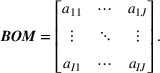
We use simulations (as in Anand et al., 2017; Balakrishnan et al., 2011) to help compare heuristics’ performances while holding all other factors constant and to gain insight into the drivers of performance. We consider a firm that uses a common set of resources to make several products with uncertain demand. As in Banker and Hughes (1994), we assume Leontief technology to map product demand distributions to resource demand distributions via a consumption matrix. Each element in this matrix is the quantity of resource i required to make one unit of product j. This mapping is akin to a BOM that translates product demand to the demand for resources. The goal is to determine the advance purchase quantity of each resource that minimizes the expected costs of meeting realized demand.

We model limited information as the firm having incomplete and imperfect knowledge of the BOM. That is, it knows the values for only a subset of rows and the known values contain measurement error. In an inventory planning context, the BOM is “fuzzy” (Guillaume et al., 2013), forcing the use of heuristics.

We examine three kinds of heuristics: ratio‐based point estimates, methods that include information about opportunity costs, and distributions fit to available data. We draw the first two methods from the practitioner literature and theoretically motivate the third approach. We examine two variations of the practice‐based methods in ways that potentially enhance performance efficiency (thus, we examine five heuristics in total). We investigate generalizability by systematically varying the quantity and quality of information available for executing the heuristics. We examine robustness by varying the parameters of the production technology and resource costs. Our major findings are as follows.

Absent measurement error, ratio‐based point estimates yield costs that are ∼109% of the costs attainable with full information. We note that these ratio‐based heuristics resemble the core feature in cost accounting systems, wherein firms model the consumption of “non‐driver” or support resources by assigning each such resource to a “driver” resource to form cost pools. The entire cost of resources in a cost pool is then allocated to products in proportion to the consumption of the driver resource. Similarly, a ratio‐based heuristic estimates the demand for a non‐driver resource as being proportional to that of a driver resource (e.g., one kitchen helper for every six waiters).

Augmenting ratio‐based heuristics by including information about opportunity costs, as in inventory planning models, increases performance measurably. Data show that this approach yields results that are comparable to the gains available from the sophisticated statistical method of directly fitting a distribution to observed historical data about resource demand.

A “dual‐driver” costing system is one in which a firm uses two drivers to model the consumption of each non‐driver resource. We find that modifying observed heuristics to include dual drivers leads to gains in cost efficiencies and that the gains are pronounced when resource costs are diffuse. This finding is consistent with the argument in Balakrishnan et al. (2004), who develop a conceptual argument, and Balakrishnan et al. (2011), who demonstrate the idea empirically, for using indexed drivers in cost accounting systems. However, data also show that information‐based approaches (i.e., including opportunity costs) dominate mechanical improvements (e.g., dual drivers).

We next examine the effects of the quality and quantity of information available to the firm on performance. With zero measurement error, increasing the precision of the information that translates the demand for driver resources to the demand for non‐driver resources (specification error in the terminology of Datar & Gupta, 1994) only has a small, albeit positive, effect. ⁴ Moreover, consistent with prior research (e.g., Balakrishnan et al., 2011), the benefit of increasing the total amount of information (i.e., knowledge about the BOM or aggregation error) tapers off rapidly. Measurement error has a large and convex impact on performance and is the dominant force.

Measurement error has a significant interaction effect with problem size and the precision of information relating driver and non‐driver resources. With sufficient measurement error (10%–15% with our set of parameters), system performance could decline as we increase the precision of available information (regarding the ratios) and/or increase the quantity of available information (the number of driver resources). Thus, our data support the theoretical conjecture that errors in cost systems offset and that improving one dimension alone might worsen performance. Taken together, these findings suggest that firms would be well‐advised to focus their efforts on refining the estimates of the demand distributions (i.e., reducing measurement error) for a handful of driver resources.

We examined alternate ways to select driver resources, given their centrality in the problem we consider. We find that a greedy algorithm of picking the most expensive resources, an approach consistent with practice, yields the best performance. This finding reinforces related results found in other contexts (e.g., Bassok et al., 1999; Biller et al., 2005).

Our findings are robust to variations in the parameters of the simulation model such as the density of the BOM matrix, methods for grouping non‐driver resources with driver resources, and the relative distribution of costs over resources.

Our findings contribute to the operations management and cost accounting literatures. We add to the operations literature on resource planning by considering the effects of limited information. We provide guidance to organizations that struggle with the consequences of an incomplete BOM (Francis et al., 2007; González et al., 2013; Peng & Nunes, 2009; Stentoft et al., 2015). We also add to the accounting literature on the design of product costing systems (Labro, 2019). Our innovation is to consider limited information in a different context—capacity planning for support resources. We find that many of our findings echo those in the product costing literature enhancing their generalizability.

MODEL

The firm

We model a one‐period firm ⁵ as a process that transforms I resources to produce J outputs. Let

$\vec{\mathcal{Q}}$

be a

$J\times 1$

vector of product demand distributions, where each element

$Q_j$

of

$\vec{\mathcal{Q}}$

is a distribution with support over

${\mathbb{R}}_{\ge 0}$

. The firm utilizes Leontief technology. Let BOM be a

$I\times J$

matrix that represents the firm's technology. Each element

$a_{ij}$

represents the number of units of resource i required to make one unit of product j.

1

Let

${\vec{q}}_t$

be a

$J\times 1$

vector of production (equal to sales) quantities of outputs. Then,

${\overrightarrow{\mathrm{TRU}}}_t$

, a

$I\times 1$

vector of total resource usage (in units of resources consumed), is

$${\overrightarrow{\mathrm{TRU}}}_t=\mathit{BOM}\times {\vec{q}}_t.$$

2

Input markets are perfectly competitive. Let

$\overrightarrow{\mathrm{RCU}}$

be a

$1\times I$

vector of constant unit prices for resources. We compute the

$I\times 1$

vector of total resource costs (in dollars)

${\overrightarrow{\mathrm{RCC}}}_t$

needed to produce mix

${\vec{q}}_t$

as ⁶

$${\overrightarrow{\mathrm{RCC}}}_t=\overrightarrow{\mathrm{RCU}}{}^T\circ {\overrightarrow{\mathrm{TRU}}}_t=\overrightarrow{\mathrm{RCU}}{}^T\circ \left(\mathit{BOM}\times {\vec{q}}_t\right).$$

3

This formulation captures settings such as a restaurant deciding on staffing levels, a bakery selling many varieties of baked goods using a recipe to estimate the ingredients needed, a manufacturer using a routing sheet to estimate machine hours needed to make its many products, and a bank using activity sheets to decide on the number of tellers. We note that the firm's operations and accounting systems will document the total consumption of each resource even if the firm does not know the usage of any given resource by a specific product. That is, these systems provide values for

${\vec{q}}_t,$

${\overrightarrow{\mathrm{TRU}}}_t,$

and

${\overrightarrow{\mathrm{RCC}}}_t,$

independent of the firm's knowledge about its BOM .

Opportunity costs

For many resources such as buildings, staffing, machinery, and raw meat in a restaurant, cost efficiencies motivate firms to purchase capacity ahead of knowing demand. Let

$r_i$

be the capacity of resource i bought ahead of knowing demand. Of course, realized demand for resource i might exceed or fall short of

$r_i$

. As each of these outcomes triggers a different opportunity cost, capacity planning trades off these two sources of opportunity costs.

Many sources shape the opportunity costs associated with overstocking (understocking) resources. Salvage values and proceeds from distress sales reduce the costs of overstocking. In a multiperiod formulation, the cost of overstocking would include holding costs. The cost of understocking includes reputational losses in addition to any contribution margin lost by not being able to meet demand. Any ability to change prices affects opportunity costs because such adjustments alter product demand and thereby affect resource demand. Finally, while firms could adjust ex post the capacity for some resources (e.g., hire temporary labor or sell unneeded materials), it is impossible to adjust the capacity of others (e.g., rooms in a hospital, seats in a movie theater, size of an oven in a bakery). The level of flexibility (i.e., the extent of hard vs. soft capacity constraints) in adjusting capacity levels ex post affects the opportunity costs of understocking resources.

To keep our focus on capacity planning, we model opportunity costs in a general way rather than consider a specific contextual setting. We follow Banker and Hughes (1994) and make three assumptions. First, firms can purchase additional capacity for any resource i at a premium price after observing realized demand. Formally, let

$c_i^u=c_i^o(1+{\theta }_i$

) where

$c_i^o$

is the unit cost of acquiring resource i in advance of demand,

$c_i^u$

is the cost of acquiring resource i on the spot market after observing realized demand, and

${\theta }_i>$

0 is the premium paid to purchase in the spot market. Second, all products are sufficiently profitable, so the firm wants to satisfy all realized demand. Third, product markets are such that price increases to lower demand are not a preferred option. With these assumptions, the magnitude of the spot premium determines the opportunity cost of understocking resource i;

$O{C}_i^u=c_i^o{\theta }_i.$

Moreover, as we assume that resources last for one period and have no salvage value, the opportunity costs of overstocking resource i is

$O{C}_i^o=c_i^o$

, the advance purchase cost of the resource.

Full information

For our benchmark setting, we assume knowledge of the entirety of the BOM ( BOM ). With this, we compute the demand distribution for each resource as

$$\vec{\mathcal{R}}=\mathit{BOM}\times \vec{\mathcal{Q}},$$

4

where

$\vec{\mathcal{R}}$

is an

$I\times 1$

vector of resource demand distributions. As noted in Equation (4), the demand distribution for a resource i is a convolution of the demand distributions for all products that use the resource. A bakery that uses the same set of resources—flour, kneading and proving time, water, sugar, additives, and time in the oven—to make many kinds of breads is a ready example. Of course, the derived resource demands could be correlated even if the product demands are uncorrelated because various products might use the same set of resources in different proportions.

Let

$F_i(·)$

be the cumulative distribution function of the demand distribution for resource i. Then, the optimal advance purchase quantity

$r_i^{\ast }$

for each resource is (Nahmias & Olsen, 2021)

$$r_i^{\ast }=F_i^{-1}\left(\frac{O{C}_i^u}{O{C}_i^u+O{C}_i^o}\right)=F_i^{-1}\left(\frac{{\theta }_i}{{\theta }_i+1}\right).$$

5

Thus, with full information, the firm can compute the optimal capacity level for every resource, that is, the first‐best capacity.

The model developed in Equations (1)–(5) is versatile and could represent many real‐world settings. For example, if the BOM contains just one element, this setting is the classic newsvendor problem. When the BOM is a diagonal matrix, the model captures settings where each product uses only one resource, and resource demands are only correlated when product demands are correlated. An example is a wholesaler stocking inventory of each of its products. Finally, the magnitude of the spot premium determines the relation between expected demand and the advance purchase quantity. The advance purchase quantity is zero if

${\theta }_i=0$

(resources bought as needed) and increases in

${\theta }_i$

.

Limited information

We introduce a role for information as the firm having imperfect and incomplete information about the matrix BOM . This assumption is realistic and is consistent with the ubiquitous use of cost systems.

Imperfect information arises because of measurement errors in estimating the pattern of resource consumption (the elements in BOM ). Such errors are more likely and greater in magnitude when the firm is considering a new service relative to altering existing technologies. They also arise because of inherent uncertainties in the production process (e.g., cooking times for the same dish vary, and yield rates are uncertain), difficulties in measuring resource use exactly (e.g., how much plastic and paper to use when packaging products), and so on. Formally, we model measurement error as

$\mathit{BO}{\mathit{M}}_{\mathit{meas}}=(\mathit{BOM}+\vec{\epsilon })$

where

$\vec{\epsilon }$

is some noise‐generating process.

Incomplete information arises because, in practice, firms know the consumption of only some resources—we term these driver resources—by product. ⁷ Resources that represent variable costs are good examples of driver resources. A manufacturer would have excellent information about the material and labor needs for each of its products. A recipe provides the input–output ratios for baked goods and helps decisions about the amount of flour to stock. The firm may also have insight into the demand for some resources shared across products. Engineers can supply the times required for machining operations, chefs can estimate cooking times, and banks can project the average mix of services in a day when determining the demand for tellers. In contrast, consumption of other resources cannot be observed on a per‐unit basis (e.g., see Anand et al., 2017; Chen‐Ritzo, 2006). These non‐driver resources are items such as the amounts of coolants required in a machine shop, tool oil used, the number of helper staff in a kitchen, the number of technicians in the maintenance department, and computing resources. We focus on how limited information influences the way firms plan the capacities for these non‐driver resources.

We operationalize driver and non‐driver resources as a firm having knowledge about the values of the elements in some, but not all, rows of the matrix BO M _meas . Rows that are observable (unobservable) correspond to driver (non‐driver) resources. Without loss of generality, let the first k resources be driver resources and the remaining

$(I-k)$

rows represent non‐driver resources. Let BO M _obs represent the portion of the matrix BO M _meas known to the firm. Formally,

$$\mathit{BO}{\mathit{M}}_{\mathit{obs}}={\mathit{I}}_{1\text{…}\mathit{k}}\times \mathit{BO}{\mathit{M}}_{meas},$$

6

where I _{1… k} represents the first k rows of the identity matrix.

The relative proportions of driver and non‐driver resources (the fraction

$k/I$

) determines the magnitude of the problem that arises from the lack of full knowledge about BOM . An increase in the ratio reduces the severity of the problem as we have information about a greater number of resources. Problem severity also decreases in the concentration of resource costs. If a few high‐value (driver) resources account for most of the costs, then the loss from not knowing information for the remaining (non‐driver) resources is reduced. In our numerical analyses, we accordingly vary these two factors to provide insight into the robustness of our findings.

Extrapolating historical information

Because of incomplete information, firms must extrapolate the information about driver resources to determine the capacities for non‐driver resources. Such extrapolation is possible if the firm has produced related products before, its existing technology is similar enough, ⁸ and/or the employees have industry knowledge or relevant human capital. In the case of innovative technology, this knowledge might just be an educated guess. This approach of extrapolating known information to fill in gaps has a striking similarity with cost accounting systems found in all organizations. These systems employ a “cost driver” (with known consumption patterns) to allocate the costs of “indirect” resources (with unknown consumption patterns) to cost objects such as products.

Of course, the precision of the information relating driver and non‐driver resources will vary across production technologies and contexts. A firm replicating an existing facility to augment capacity would have excellent information on the relation between resource configurations and usage. Building a newer model using data from an existing application (as in making a next generation of a camera or car) or implementing the next generation of technology (as in making electronic chips) will erode precision. Input from industry experts could help increase accuracy. ⁹ An experienced restauranter can generate an excellent estimate of the number of waitstaff needed when provided with the number of tables and the target service level.

As with opportunity costs, we take a simple approach to model the information that relates driver and non‐driver resources. For a past period, the firm will know realized demand for its products. Accounting records provide the aggregate amounts of each resource consumed. Thus, the firm can compute ratios that relate the consumption of all pairs of driver and non‐driver resources. If it has data for many periods, the firm will have a distribution of the ratio for each pair. These ratios will differ across periods because of variations in realized demand for the products and thus the consumption of resources. The firm could use a summary statistic such as the mean of the distribution of ratios or use other statistical methods to estimate the “true” ratio of relative consumptions.

Formally, we suppose that a firm maintains a database of past product demand vectors, q ^hist (see Equation 7) and corresponding resource consumption vectors TR U ^hist . The values in these vectors are observable to the firm through their accounting system, regardless of the extent of knowledge of BOM . Equation (8) shows the theoretical relationship between q ^hist and TR U ^hist . The dimensions of these matrices are

$J\times n$

and

$I\times n$

, where I is the number of resources employed by the firm in the production of its J outputs, and history has n periods. Over time, the firm builds a history of

${\overrightarrow{\mathrm{TRU}}}_t$

and

${\overrightarrow{\mathrm{RCC}}}_t$

vectors and can compute correlations and resource ratios.

7

$${\mathit{TRU}}^{\mathit{hist}}=\mathit{BOM}\times {\mathit{q}}^{\mathit{hist}}.$$

8

We chose this model of information precision because it helps us emphasize the links between accounting information and resource planning. The informational foundations of this approach are consistent with practice and with financial accounting. Specifically, because they expend money to acquire specific resources, firms observe the consumption of each non‐driver resource in the aggregate after production has occurred. A firm would know that it consumed 1.3 megawatts of electricity even if it does not know the electricity consumption by product. Stated differently, even though the firm can only observe some rows of BOM , it can still observe the total consumption of resources (i.e.,

${\overrightarrow{\mathrm{TRU}}}_t$

and

${\overrightarrow{\mathrm{RCC}}}_t$

) for a given production decision

${\vec{q}}_t$

. Also, we can directly manipulate the precision of the information relating driver and non‐driver resources by varying the length of history, n.

In sum, we characterize the limitations in available information along three dimensions. The ratio of driver resource cost to total resource cost defines the scope of the problem (i.e., the amount of available information) in planning the capacities of non‐driver resources. Measurement error relates to the confidence we have in our estimates of how products use driver resources. Finally, precision is the confidence we have in our estimates of the relation between the usage of driver and non‐driver resources.

Heuristics considered

We consider five heuristics for choosing the capacity levels of non‐driver resources. We choose two from practice. We develop two that seek to improve on practice‐based approaches and construct one based on theory.

Heuristics 1 and 2: Point estimates with one or more drivers

In our model, the firm's accounting system provides the values in the vector TR U ^hist . The firm can use this knowledge to compute the relative use of non‐driver and driver resources. The idea is that a firm could rely on history to infer that, on average, it needs one supervisor for every seven workers or 1200 machine hours. In other words, it can compute the historical ratios of consumption of non‐driver resources to driver resources. Then, once it determines the capacity level of a driver resource, it can use the relevant ratio to determine the amount of capacity to purchase for the corresponding non‐driver resource. Such a point estimate with one driver, the Point1 heuristic, is widely used in practice. Formally, using the firm's resource demand history, for each non‐driver resource i in a cost pool, we compute the ratio r ₁ between consumption of non‐driver resource i and its driver resource

$d_1^{\ast }$

. We multiply the advance purchase quantity of

$d_1^{\ast }$

by r ₁ to obtain the advance purchase quantity of resource i.

The use of indexed drivers in cost accounting (e.g., Babad & Balachandran, 1993; Balakrishnan et al., 2011; Homburg, 2001) motivates the improvement proposed in the Point2 heuristic. An indexed or synthetic driver is the weighted average of the allocation percentages from two or more primitive cost drivers. For example, we could allocate tooling costs using a synthetic driver that averages machine hours and labor hours. In the context of capacity planning, this refinement is akin to using both the magnitude and the intensity of use (e.g., size of a dorm in square feet and the number of students to estimate the needs for janitorial staff). That is, we use the ratios from multiple driver resources to “triangulate” the purchase quantity of the non‐driver resource. Let r ₁ be the ratio between the consumption of a non‐driver resource and to that of driver resource #1, for which the firm optimally acquires

$d_1^{\ast }$

units. Let r ₂ and

$d_2^{\ast }$

be the corresponding values for the same non‐driver resource and driver resource #2. Using triangulation, the firm would acquire

$\frac{r_1{d}_1^{\ast }+r_2{d}_2^{\ast }}{2}$

units of the non‐driver resource.

Heuristics 3 and 4: Incorporate information about opportunity costs, with one or more drivers

The point heuristics ignore information about the opportunity costs associated with non‐driver resources, which firms typically possess. Thus, we explore the gain from including this information in a heuristic. Observed stocking policies support the inclusion of opportunity costs into capacity planning. Firms buy resources with small spot market premiums (e.g., oils and coolants, wood glue for a cabinet maker) on an as‐needed basis. In contrast, they plan for “unused capacity” in resources such as design engineering time that are harder to augment on an as‐needed basis. At an extreme, a two‐bin strategy is a prudent way to have large stocks of low cost but critical items that are not easily replenished (e.g., specialized screws used in electronic equipment such as mobile phones).

In the Dist1 heuristic, we derive a distribution for the non‐driver resource as a transformation of the demand distribution for the relevant driver resource. Suppose the demand for a driver resource follows some distribution

$\mathcal{D}$

:

${\mathcal{R}}_i\sim \mathcal{D}(\mu ,{\sigma }^2)$

. Let β be the ratio between a non‐driver resource and the driver resource (as calculated for the Point1 heuristic). Then the implied distribution for the non‐driver resource is

$\beta ·{\mathcal{R}}_i\sim \mathcal{D}(\beta \mu ,{\beta }^2{\sigma }^2)$

. We then apply the newsvendor model with the component‐specific critical ratio,

$(\frac{{\theta }_i}{{\theta }_i+1}),$

to the derived distribution of each non‐driver resource to compute the capacity level for that resource.

As with the point ratios above, the firm could improve or triangulate using multiple driver resources (i.e., compute two implied demand distributions). For the Dist2 heuristic, we compute the quantity for a non‐driver resource using two different driver resources by solving the newsvendor problem for each, independently. We average the two solutions to determine the quantity to acquire.

Heuristic 5: Fit a distribution

The point and the derived distribution heuristics require that the firm specify at least one driver resource for each non‐driver resource. That is, these heuristics require the firm to form cost pools by associating every non‐driver resource with a driver resource. The distribution heuristic also limits the distribution to be a transformation of the associated driver demand distribution. Theory offers a way to relax both requirements with sufficient data on the firm's history. Using the vector of realized demand for each non‐driver resource, the firm could use a distribution fitting method, such as kernel density estimation (KDE), to directly estimate the distribution of each non‐driver resource. Of course, the firm must specify the functional form of the distribution to be fitted, and the number of available observations influences the quality of the fit. It can then formulate and solve a newsvendor problem, employing the resource‐specific costs of advance and premium purchases.

SIMULATION PROTOCOL

We conduct a simulation to ascertain the efficiency of the heuristics described earlier. A simulation is appropriate here because, given the interlinked nature of resource consumption, the equations of this system cannot be solved in closed form (Anand et al., 2017). Additionally, the simulation permits flexibility in parameter choices, allowing us to model a wide range of parameter combinations.

Setup

We define a firm by (1) a set of products it makes and a known demand distribution for each; (2) a set of resources, as well as the pre‐production unit cost of each resource and a premium for spot purchases; and (3) a consumption or BOM matrix that maps the number of units of each resource required to make one unit of each product. For each firm, we hold items 1−3 constant.

We create a random sample of 1000 firms. Each firm sells 20 products, with normally distributed and independent demands. For each product, we draw the mean demand from discrete U(10, 40) multiplied by a randomly chosen integer from discrete U(3, 10). We draw the coefficient of variation from U(0.1, 0.3) and multiply it by the mean to obtain the standard deviation. This method for choosing the parameters permits realized demand to be positive with better than 99% probability.

Each firm has 50 resources in total, and each product uses a subset of these resources. The BOM matrix maps product demand to resource demand. We follow the procedure in Anand et al. (2019) to create a BOM for each firm. This BOM satisfies the following properties.

We randomly choose a resource density parameter, the percentage of cells with a non‐zero entry, from

$U(0.4,0.7).$

This parameter determines the density (alternatively, sparsity) of the BOM . A sparse matrix, with many zero values as cell entries, resembles consumption patterns in a job shop in which each product consumes a distinct set of resources. A dense matrix resembles a process shop in which most products follow a similar production process and consume the same resources but in different proportions. The imposed distribution of the density parameter leads to virtually all products using only a subset of resources.

We require that each product consumes at least one resource and that each resource is consumed by at least one product (i.e., no rows or columns are all zero in the BOM matrix).

Based on producing mean demand, we impute resource costs so that the spending on the top 10 resources accounts for a percentage of the total spending (i.e., resource cost dispersion) that is drawn from

$U(0.4,0.7)$

.

Given the values for resource density and the dispersion in resource costs, and the production constraints, we follow the method in Balakrishnan et al. (2011) to determine the individual cell entries in the BOM .

We draw the spot purchase premium for each resource from

$U(1.25,2.75)$

, meaning that the premium is between 25% and 175%. The impact of errors in capacity planning on total cost increases in the magnitude of the spot premium. For instance, a resource with zero spot premium would be bought on an as‐needed basis. A resource with infinite premium presents a “hard” capacity constraint, triggering the need to allocate available capacity among products, considering realized demand and contribution margins.

Table 1 supplies descriptive statistics that contextualize the above environments. The average product uses 28.1 of the 50 possible resources, with a range from 11 to 45 resources (untabulated). Likewise, the average resource is used by 11.2 of the 20 possible products, with a range from 1 to 20 (untabulated). We find limited evidence of co‐movement in resource usage at the product level. We compute pair‐wise correlation (across products or rows of the BOM ) in resource usage and average them across all resources. The reported absolute values are about 19%, which casts doubt on the use of driver resource capacities to plan for non‐driver resources (the raw average is less than 3% [untabulated], indicating the presence of large positive and negative correlations in usage). However, a different pattern emerges when we compute resource correlations empirically. When we compute resource correlations from 10,000 draws from the underlying product demand distributions, we find the correlation is about 40% (absolute values of the measure are similar in magnitude, indicating co‐movement in aggregate resource usage). Finally, the values for the standard deviation in resource costs (as computed in the full‐information solution) validate that our data permit variation in the composition of resource costs.

TABLE 1

Descriptive statistics: Bill of materials.

	Low density	Medium density	High density	Global average
	40%–50%	50%–60%	60%–70%	40%–70%
High resource cost dispersion (% cost from 10 most expensive resources = 40%–50%)
Number of resources used by average product	23.2	28.3	32.9	28.3
Average number of products using a resource	9.3	11.3	13.1	11.3
Abs. avg. pair‐wise correlation among resources	0.1907	0.1921	0.1947	0.1926
Average correlation in total consumption	0.3317	0.3993	0.4699	0.4024
Std. deviation in resource cost	$156,650	$157,684	$160,766	$158,457
Medium resource cost dispersion (% cost from 10 most expensive resources = 50%–60%)
Number of resources used by average product	23.0	28.1	32.8	27.9
Average number of products using a resource	9.2	11.2	13.1	11.2
Abs. avg. pair‐wise correlation among resources	0.1915	0.1921	0.1931	0.1922
Average correlation in total consumption	0.3250	0.4001	0.4680	0.3970
Std. deviation in resource cost	$217,554	$219,916	$220,431	$219,327
Low resource cost dispersion (% cost from 10 most expensive resources = 60%–70%)
Number of resources used by average product	23.5	28.3	33.1	28.2
Average number of products using a resource	9.4	11.3	13.2	11.3
Abs. avg. pair‐wise correlation among resources	0.1910	0.1928	0.1918	0.1918
Average correlation in total consumption	0.3317	0.4045	0.4661	0.3992
Std. deviation in resource cost	$275,227	$286,298	$278,781	$279,869
Global average (% cost from 10 most expensive resources = 40%–70%)
Number of resources used by average product	23.2	28.2	32.9	28.1
Average number of products using a resource	9.3	11.3	13.2	11.2
Abs. avg. pair‐wise correlation among resources	0.1911	0.1923	0.1933	0.1922
Average correlation in total consumption	0.3296	0.4012	0.4681	0.3996
Std. deviation in resource cost	$217,689	$221,586	$218,201	$219,157

Note: This table provides descriptive data about the BOM ( BOM ) matrix. We partition the 1000 firms in our sample along two dimensions. First, we consider the density of the matrix (percentage of cells with positive entries) and divide the sample into terciles. Second, we consider the percent of costs from the 10 most expensive resources (computed using mean demand for all products) and again divide the sample into terciles. Note that high (low) cost dispersion implies that the top 10 resources account for a smaller (larger) percentage of the total cost.

Number of resources used by average product (Average number of products using a resource) is the average number of non‐zero entries in each column (row) of the BOM matrix. We compute the average pair‐wise correlation among resources as the average of the absolute pair‐wise correlation in usage, across products. That is, we compute the correlation between every pair of rows of the BOM and average over all pairs to obtain the value for a firm. We compute average correlation in total consumption by computing total demand for each resource for 10,000 random draws from the product demand distributions. We then compute pair‐wise correlations and average to determine a firm‐level estimate. We compute the standard deviation of the costs of the 50 resources when producing mean demand for all products. Lower values indicate a firm with many equally valuable resources. All entries in this table average the firm‐level value for the relevant measure over 1000 firms.

In sum, we allow for a wide variation in base parameters. ¹⁰ Moreover, the range of parameters we employ is identical to that employed in prior research (Anand et al., 2017, 2019; Balakrishnan et al., 2011), which has employed a similar methodology.

Full‐information solution (first best)

Using the vector of product demand distributions

$\stackrel{\sim }{\mathcal{Q}}$

, we compute the vector of resource demand distributions as

$\stackrel{\sim }{\mathcal{R}}=\mathit{BOM}\times \stackrel{\sim }{\mathcal{Q}}$

(as per Equation 4). We solve a newsvendor problem independently for each resource to obtain the vector of optimal advance purchase quantities. Recall that the opportunity cost of overstocking,

$O{C}_i^o$

, is the unit cost of the resource i, and the opportunity cost for understocking,

$O{C}_i^u$

, is the spot premium for that resource.

For each firm, we compute the total advance capacity cost, expected spot capacity cost, expected spot premium paid, and expected cost of supply–demand mismatch (expected cost of spot purchases plus expected cost of leftover inventory). These are the “first best” or full‐information costs that serve as the benchmarks for later comparisons.

Limiting available information

For each of the 1000 simulated firms, we manipulate three items: the number of driver resources, which determines the scope of the information problem; the magnitude of measurement error in estimating the usage of driver resources; and the length of history that influences the precision of the information that relates driver to non‐driver resources.

We vary the number of driver resources at three levels: three, five, and 10. The greater the number of driver resources, the less severe the firm's information problem because the number of non‐driver resources decreases to 47, 45, and 40 (all firms have exactly 50 resources). We often refer to the number of driver resources as the number of cost pools. Surveys show that most firms have fewer than 20 drivers (Babad & Balachandran, 1993).

We vary the extent of measurement error in estimating the usage of driver resources at four levels. We randomly add measurement error (as a percent of the true value) drawn from a uniform distribution with supports over (0%, ±5%, ±10%, and ±15%). Thus, the reported consumption of a driver resource by the firm's products is a noisy function of the actual consumption.

We operationalize information precision as the length of the firm's history, which we vary at four levels: (

$n=$

5, 10, 25, or 50 periods). The longer the history, the greater is the precision of the ratio that relates the consumption of the driver resource to the non‐driver resource. We make n draws from the firm's product demand distribution vector and use that to compute the history of resource demand. We then compute the empirically observable correlations in aggregate resource use (see Table 1), as well as the ratios between driver and non‐driver resources.

Together, we consider 48 (=3 * 4 * 4) information environments for each of our sample firms.

Solving for installed resource capacity

For each driver resource, the distribution of demand is known. We compute

${\vec{\mathcal{R}}}_{obs}$

, the vector of demand distributions for driver resources, as

9

where

$\vec{\mathcal{Q}}$

is the vector of product demand distributions. We solve the associated newsvendor problems to determine the optimal advance purchase quantities for driver resources. The derived solution corresponds to the full‐information solution when there is zero measurement error in the consumption quantities. Measurement error in the relevant rows (i.e., cell entries in

$\mathit{BO}{\mathit{M}}_{meas}$

differ from those in BOM ) will cause the installed capacity to differ from the first‐best values.

Turning to non‐driver resources, the Point1 and Dist1 heuristics associate each non‐driver resource with a driver resource. That is, we form a cost pool that comprised a driver resource and associated non‐driver resources. We use a National Football League (NFL) type draft system to assign non‐driver resources to cost pools. Each cost pool takes a turn and chooses the non‐driver resource with the highest correlation from the remaining unassigned non‐driver resources. This process repeats until we assign all non‐driver resources to a cost pool. For the Point2 and Dist2 heuristics, we need to add a second driver. For each non‐driver resource, we choose from the remaining driver resources the one with the highest correlation in usage. We compute the capacity for the non‐driver resource for both driver resources and average the values. We examine alternate methods (e.g., use stepwise regression, random assignment) in robustness tests reported later. The KDE method does not require the formation of cost pools as we fit a distribution directly to the history of usage for each non‐driver resource.

Evaluation of solutions

Our benchmark for evaluating the efficacy of a heuristic is the expected cost under full information, when the firm has complete and perfect information about BOM , and hence about resource consumption by each of its products. We compare the expected cost using each heuristic to its benchmark value to determine the heuristic's relative efficacy.

We examine generalizability by manipulating the information environment along select dimensions: the proportion of driver to non‐driver resources (quantity of available information), the extent of measurement error in the consumption of driver resources (quality), and the length of history available (precision). We evaluate robustness by varying the methods for choosing driver resources and for grouping non‐driver resources with driver resources, the density of the BOM matrix, the dispersion in resource costs, and the distribution of resource spot premium.

For each firm and combination of information limitations, we compute the advance purchase capacity cost, the expected value of spot premium paid, and the expected cost of supply–demand mismatch (expected cost of spot purchases plus expected cost of leftover inventory). The efficiency of any given heuristic is the “cost ratio” obtained relative to the same value computed under full information. It is sufficient to examine costs in lieu of revenues or profits because all products are profitable. This approach also avoids scaling issues that can arise when profits are small and used in the denominators of ratios.

Our primary dependent variable is the expected cost of supply–demand mismatch, which is computed as the sum of the expected cost of spot purchases and the expected cost of leftover inventory (e.g., see Zhao et al., 2012). This cost is positive, even with full information because of the uncertainty in product demand. Then the cost ratio is the cost of supply–demand mismatch under a specified information limitation (e.g., number of drivers = 3, length of history = 10, measurement error = 0%) divided by the value obtained with full information for that firm. The use of a ratio as a measure of efficacy has the advantage that parameter choices affect both the full‐information (first best) and the heuristic‐based (second‐best) solution. Thus, we expect our inferences to be robust to parameter choices such as the relative ratios of the opportunity costs of under‐ and over‐stocking, the demand distribution, and features of the production function. ¹¹

Inferences from other dependent variables, such as the ratio of expected total cost of supplying demand, are similar. Detailed results are available on request.

Number of observations

As noted earlier, for each firm, we vary the information available along three dimensions: the number of driver resources at three levels; the error in measuring the usage of driver resources at four levels, and the length of history at four levels to obtain 48 configurations for each firm. For each of these 48 configurations, we apply five heuristics, giving us 240 observations for each firm. We repeat the process for 1000 firms (with random choices for the density of the BOM and the concentration in resource costs) to obtain 240,000 observations. We also have the full‐information solution for each of the 1000 firms.

RESULTS

We present results in the form of graphs and tables that aggregate and sort the observations along the dimensions of interest. We do not present formal statistical analyses as sample size, and hence statistical significance can be increased arbitrarily in a simulation (Anand et al., 2019). We provide additional data in the Online Appendix, labeling the relevant tables and figures with the prefix A.

Ratio‐based planning is robust and efficient

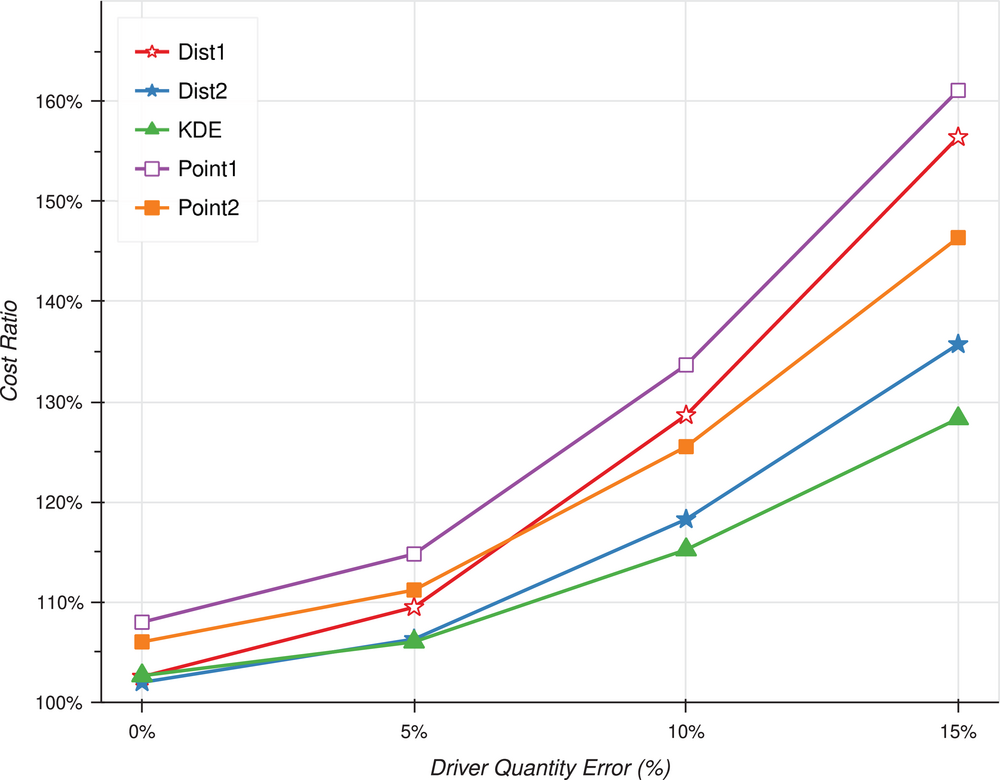
In Figure 1, we plot the efficiency of heuristics that plan the capacity of non‐driver resources. The x‐axis is the number of driver resources considered and the y‐axis is the cost ratio, with each plot marker averaged over 4000 observations. We set measurement error to zero as it has significant interactive effects, discussed later.

FIGURE 1

Efficiency of heuristics as knowledge of bill of material increases, 0% measurement error. For each of 1000 simulated firms, we infer the demand distribution for each of its 50 resources from the known demand distributions for each of its 20 products. We solve a newsvendor problem independently for each resource and obtain the optimal advance purchase quantity for each resource. From this, we compute the first‐best expected cost of supply–demand mismatch as the sum of the expected cost of spot purchases plus the expected cost of leftover inventory. We manipulate the length of history for each firm at five, 10, 25, or 50 periods. For each period in the firm's history, the firm knows the aggregate consumption of each resource required to meet product demand. From the resource consumption history, the firm computes the pair‐wise ratio of resource consumption between all resources. In this figure, we assume zero measurement error in resource consumption. For each level of the length of history, we manipulate the number of driver resources for which the firm has full information about the consumption of the resource by product. We use each driver to form a cost pool and assign non‐driver resources based on correlation patterns. We employ five heuristics to determine the advance purchase capacity of the non‐driver resources. Under the Point1 heuristic, the capacity level of a non‐driver resource equals the optimal capacity for the corresponding driver times the historical ratio between the driver and non‐driver resource. Under the Dist1 heuristic, we scale the demand distribution for the corresponding driver by the ratio and solve a newsvendor problem using the under‐ and over‐stocking cost of the non‐driver resource. Under the kernel density estimation (KDE) method, we estimate a distribution separately for each non‐driver resource from its history. For each firm, length of history, number of driver resources, and heuristic, we compute the total expected cost of supply–demand mismatch across all resources and divide it by the corresponding first‐best cost to obtain a cost ratio. The figure shows the cost ratio for each condition, averaged across levels of the length of history. Each data point corresponds to 4000 observations.

On average, the Point1 heuristic increases total cost by ∼9% relative to a solution with full information in an informationally sparse setting with three driver resources and 47 non‐driver resources. Violin plots (see Figure A1) reveal many outliers. The top decile of cost ratios averages 122% (max value = 158%, untabulated), and these observations have a greater likelihood of occurring in settings with high resource cost dispersion. ¹² Increasing the number of drivers improves the average cost ratio and reduces the variance in a concave fashion (see also Table A1). This finding, which is consistent with and augments (for variances) prior research that reaches a similar conclusion in different contexts, corroborates practice recommendations to restrict the number of driver resources. ¹³

Data in Table 2 provide insight. First, as expected, the percentage of costs accounted for by driver resources increases as we classify more inputs into this category. The ratio is 36.8% with three driver resources and 55.2% with 10 driver resources. Naturally, the costs from incorrect planning for non‐driver resources monotonically decline. Moreover, the percent increase in costs is concave, meaning that the reduction in the scope of the problem is also concave, limiting the gain from adding more drivers. Next, considering five driver resources, the average correlation in total resource usage within a cost pool is 0.5501, noticeably higher than the overall average of 0.3996 reported in Table 1. The implication is that the practice of forming cost pools by looking at correlations in resource usage leads to a significant information gain when planning for non‐driver resources. The final row of Table 2 reports on the accuracy of the ratio relating driver to non‐driver resources. We find that the average absolute error is about 3.6%. Together, the data show that increasing the number of pools helps both by reducing the magnitude of the problem and by increasing the within‐pool correlation, which in turn increases the accuracy of the ratio used in the heuristic.

TABLE 2

Effect of number of driver resources on quality of available information, 0% measurement error.

	Number of driver resources
	3	5	10	Global average
Percent of total cost contained in driver resources (in first‐best solution)	36.8%	43.3%	55.2%	45.1%
Average pair‐wise correlation in resource usage of driver and non‐driver resources within a cost pool (determined from BOM)	0.2181	0.2297	0.2468	0.2315
Average correlation in total consumption of driver and non‐driver resources within a cost pool (empirically determined)	0.5328	0.5501	0.5734	0.5521
Mean absolute percent error in installed capacity for non‐driver resources (Point1 heuristic, length of history = 10 periods, 0% measurement error)	3.57%	3.63%	3.62%	3.61%

Note: This table shows the effect of increasing available information on sources of error in capacity planning when there is 0% measurement error in driver resources. As the number of driver resources increases, firms’ knowledge of their BOM increases. Percent of total cost contained in driver resources is the percent of total cost accounted for by driver resources when the firm purchases the optimal quantity for every resource (first best). Average pair‐wise correlation in resource usage of driver and non‐driver resources within a cost pool (determined from BOM) is computed as follows. Within a cost pool, the pair‐wise correlation between the pool driver and every non‐driver is computed using rows of the BOM. This is averaged across all non‐driver resources. Average correlation in total consumption of driver and non‐driver resources within a cost pool (empirically determined) is computed similarly, but instead of using rows of the BOM, 10,000 draws from the resource demand distributions are used. Mean absolute percent error in installed capacity for non‐driver resources is ABS [(second best capacity – first best capacity)/first best capacity], averaged across all non‐driver resources. Second best capacity is computed using a heuristic, while first best is computed using full information. Larger values of this variable indicate lower quality of the ratios that map driver resources to non‐driver resources. This measure is reported only for the Point1 heuristic, length of history of 10 periods, and 0% measurement error. Entries in this table average the firm‐level value for the relevant measure over 1000 firms.

Returning to Figure 1, we find that adding in data about resource‐specific opportunity costs (Dist1) reduces the average cost ratio from 109% to 103% with three driver resources. This refinement is implementable as firms likely have good information about the unit costs and spot premiums for resources. As noted earlier, observed stocking policies for support resources appear to employ estimates of opportunity costs. Compared to Point1, the Dist1 heuristic has lower variance and fewer outliers (the average is 110% for the top decile of cost ratios and a maximum of 139%; see Figure A1). The average improvement, relative to the solution from the Point1 heuristic, ranges from 1.2% for the bottom decile to 13.6% for the top decile (see Table A2 and Figure A2). Moreover, the improvement obtains in over 99% of examined cases. The larger differences are more likely in settings with diffuse resource costs and higher variance in spot premiums. The mean value for DISP, the cost in the 10 most expensive resources is 51% (58%) in the top (bottom) decile of observations, sorted by the improvement in the cost ratio. Likewise, the correlation between the variance in the firm‐level spot premium and the gain from including opportunity costs is 0.24 (p < 0.001).

Data show limited incremental gains from increasing statistical sophistication. Fitting a distribution to the observed history of usage of non‐driver resources (KDE) does not outperform the simpler approach in the Dist1 heuristic.

We find similar patterns when we consider the length of history rather than the number of drivers (Figure A3). Firms do not appear to need deep information or experience with a proposed technology to make good planning decisions. Overall, we conclude that simple, easily implemented heuristics are cost‐efficient ways to address information limitations.

Finding 1 : Using historical ratios of the capacities of non‐driver to driver resources (“capacity ratios”) leads to a solution that is ∼9% more expensive than the full‐information solution, in the absence of measurement error. The gain from increasing the number of driver resources or the precision of available information is concave. Reliable gains are obtained from including information about opportunity costs of non‐driver resources, particularly when resource costs are diffuse.

Using multiple drivers to triangulate increases cost efficiency

Figure 1 also shows significant gains from the refinement of using two drivers to estimate the usage of capacity resources. Adding the estimate from another driver (with lower correlation) and averaging the two results decreases the cost ratio from 109% (Point1) to 107% (Point2) when using three cost drivers; the gains are similar with five and 10 cost drivers, indicating that the triangulation manipulation produces a main effect. We also document a reduction in the variance of the cost ratio, suggesting that the improvement has bite in a variety of settings (see Figure A1). However, the gain is not guaranteed as we fail to document an improvement in about 5% of the cases.

We find a similar pattern for Dist1, a heuristic that incorporates opportunity costs. However, the decline in the cost ratio is smaller: 103% (Dist1) to 102.4% (Dist2) in the case with three cost drivers. We draw three inferences. First, the data are consistent with Balakrishnan et al. (2011) who advocate the use of indexed drivers to better measure the economic usage of resources. Even considering information costs, Homburg (2001) shows that it is often beneficial to replace a driver with a combination of other drivers. Second, triangulation (or indexing) leads to smaller gains with the more sophisticated method than the simpler method. Finally, while triangulation helps, it is better to implement heuristics that include additional information such as opportunity costs of non‐driver resources, even if they involve more computations. Both refinements have the greatest impact with diffuse resource costs, increasing the dollar magnitude of the problem of planning for non‐driver resources.

Data in Table 3 report the incremental gain in regions sorted by problem parameters. Once again, diffusion in resource costs, which directly affects the magnitude of the problem, has the largest effect. Even so, the variation in the gains due to improvements is modest. We conclude that our Findings 1 and 2 apply in general (see also Table A2 and Figure A4 in the Online Appendix).

TABLE 3

Performance of heuristics and improvements, sorted by parameter values, 0% measurement error.

			Density of BOM (DNS is % of cells with positive entry in BOM)
			High	Low	Total
Dispersion in resource costs (DISP is percent of costs accounted for by 10 most expensive resources)	Low	Point1	106.97%	107.11%	107.04%
		Point2	105.34%	105.36%	105.35%
		Dist1	102.08%	102.45%	102.84%
		Dist2	101.65%	101.91%	102.21%
		P1_P2	1.63%	1.75%	1.69%
		P1_D1	4.89%	4.66%	4.77%
		DNS	62.68%	48.05%	55.01%
		DISP	62.58%	61.97%	62.26%
	High	Point1	108.67%	109.27%	108.96%
		Point2	106.44%	107.02%	106.71%
		Dist1	102.54%	103.17%	102.27%
		Dist2	101.95%	102.49%	101.79%
		P1_P2	2.24%	2.26%	2.25%
		P1_D1	6.13%	6.11%	6.12%
		DNS	62.69%	47.58%	55.50%
		DISP	47.23%	47.06%	47.15%
	Total	Point1	107.86%	108.14%	108.00%
		Point2	105.92%	106.15%	106.03%
		Dist1	102.32%	102.79%	102.56%
		Dist2	101.81%	102.19%	102.00%
		P1_P2	1.95%	1.99%	1.97%
		P1_D1	5.54%	5.35%	5.44%
		DNS	62.68%	47.83%	55.25%
		DISP	54.54%	54.87%	54.70%

Note: This table shows the variation in the performances of the heuristics across the parameter space. We form four quadrants sorted by the density of the BOM matrix and the dispersion in the resource costs, sorting based on median values. We report values when there is 0% measurement error in driver resources and average values across the number of driver resources and the length of history. The variable P1_D1 shows the improvement from the Point1 to the Dist1 heuristic. The variable P1_P2 represents the improvement from using two drivers relative to one for the Point method, and the variable D1_D2 provides the equivalent improvement under the Dist method. DNS and DISP report the average value for the density of the BOM matrix and the percentage of cost accounted for by the 10 most expensive resources, for each quadrant. Each entry in the table is an average of the firm‐level value for the relevant measure over 1000 firms.

We investigate the gains from additional triangulation by extending the analysis to three, four, and five drivers. In untabulated results, we find that the gains, while positive, fall off sharply. Our findings suggest that averaging results from two drivers is an effective way to reduce the deleterious effects of specification error (Datar & Gupta, 1994), particularly when we consider information‐related costs.

Finding 2: Averaging the solution from two driver resources (triangulation) is beneficial in the absence of measurement error. The gain is concave in the number of additional drivers considered and in the sophistication of the heuristic. The gain applies to both job and process‐shop‐type industries. Finally, emphasizing the limits of mechanical approaches, the gain from including additional information exceeds the gain from triangulation.

Reducing measurement error in usage of driver resources is valuable

As shown in Figure 2 (see also Figure A5), measurement error has a significant and convex effect on the average cost ratio, and its variance, for all five heuristics. One implication is that it is useful to focus refinement on reducing measurement error. It is better to get good data on a few driver resources than gathering mediocre data on many driver resources. ¹⁴ For instance, considering the Point1 heuristic, the cost ratio is 135% with five pools and 10% measurement error, compared to 160% with 10 pools and 15% measurement error (see Table A4). This result echoes similar findings obtain in other contexts. Considering the stocking of operating rooms in hospitals, Rappold et al. (2011) find that reducing the uncertainty (i.e., measurement error) in the physician‐determined BOM through standardization exhibited the greatest potential for savings.

FIGURE 2

Effect of measurement error. For each firm, length of history, number of driver resources, heuristic, and level of measurement noise in driver resources, we compute the total expected cost of supply–demand mismatch across all resources and divide it by the corresponding first‐best cost, computed without measurement noise, to obtain a cost ratio. The figure shows the cost ratio for each condition, averaged across all levels of the number of driver resources and length of history. Each data point has 12,000 observations. See Figure 1 for definitions of terms and description of the method.

With high measurement error, the ordering of the heuristics is not monotonic as the negative effect of measurement error is larger for more computationally intensive methods. With zero measurement error, at 103%, the cost ratio for Dist1 is four percentage points lower than the ratio for the Point2 heuristic. However, the relation reverses (i.e., Dist1 has a higher cost ratio at 158% vs. 145% for the Point2 heuristic) when we consider a setting with 15% measurement error (see Table A3). This reversal implies that triangulation becomes attractive in settings where it might be expensive to reduce measurement error directly. The intuition is that measurement error affects both the mean and the variance of the derived resource demand distribution. While the effect of the mean affects the efficacy of both the Point and the Dist heuristics, changes in the variance only affect results under the Dist1 heuristic.

Measurement error also has a larger impact on the cost ratio than the effect from the precision of available information. In Table A6, we report the extent of absolute deviation in the installed capacity of non‐driver resources, relative to the value in the full‐information solution, sorted by the levels of precision and measurement error (for the case of five driver resources). Considering the global averages, for the Point1 heuristic, increasing the length of history from five to 50 periods reduces the error from 5.92% to 5.22%. However, the deviation from the benchmark capacity increases faster, from 4.56% to 8.14%, as measurement error increases from 0% to 15%. The intuition is that a heuristic does not consider the error in the data it uses. Measurement error affects the installed capacity for driver resources and the error flows through to non‐driver resources as well. ¹⁵ In contrast, the length of history (precision) has no effect on the capacity planned for driver resources as we assume the firm knows the demand distributions of these resources.

Finding 3: It is more important to improve the accuracy of the information about driver resources than it is to collect data for more resources and/or refine estimates of the relation between driver and non‐driver resources. The intuition is that measurement error affects the installed capacity for driver resources in addition to the solutions for non‐driver resources.

Partial improvements can hurt in settings with high measurement error

Measurement error has a significant interaction effect. For the Point1 heuristic with 15% measurement error, the cost ratio declines (from 162.1% to 161.1% to 160.1%) as we go from three to five to 10 driver resources (see Table A4). This decline is proportionately smaller than for the case with 0% measurement error, suggesting the interaction. Moreover, this interactive effect is stronger for the Dist1 heuristic. In this case, we know from Figure 1 (0% measurement error) that increasing the number of drivers decreases the cost ratio. However, this improvement is absent (and reverses to a small degree) with significant measurement error; the cost ratio changes from 156.7% to 156.1% to 156.4% as we go from three to five to 10 drivers (see Table A3). With high measurement error, we document a monotonic increase in the average cost ratio for the Point2 (145% to 146% to 147%) and Dist2 (from 133% to 135% to 138%) heuristics as we increase the number of pools from three to five to 10 (see Table A3). These findings reaffirm the earlier inference that measurement error has a larger impact on more sophisticated heuristics. As measurement error is more likely in newer firms or firms using newer technologies, such firms may be better off using simple heuristics.

We next explore settings wherein the negative effects of measurement error are pronounced. Even for the Point1 heuristic, where the average improves, the change in the cost ratio from three to five cost pools is negative for ∼49% of observations, indicating that this effect is common. For insight, we sorted the change in the cost ratio by moving from three to five drivers into deciles (Table A5). We find that the lowest and the highest deciles obtain in settings with high density for the BOM . This pattern suggests that overall error decreases (increases) if the measurement errors in the added drivers offset (accentuate) the effects of the error in the current drivers. These patterns are consistent with the argument in Datar and Gupta (1994) that selective improvement in system design (e.g., increasing the number of cost pools to reduce aggregation error) might backfire because of its interaction with measurement error. The suggestion to combat the negative effects of measurement error by using fewer cost pools is salient in setting with significant commonality in resource usage.

In Figure 3, we also consider diverse levels for the precision of available information. Data show the intuitive effects with 0% measurement error. Improving the number of drivers or the precision of available data (reducing aggregation or specification error) helps system performance. Moreover, with 0% measurement error, we do not discern a strong interaction effect between these two factors, for either of the two heuristics we consider. The story changes with significant measurement error. First, improving precision does not always help. For the Point1 heuristic with three or five drivers, cost ratio increases as precision increases. The error due to measurement, in both driver and non‐driver resources, overwhelms the marginal gain due to precision, which only affects non‐driver resources. ¹⁶ Likewise, considering the Dist1 heuristic, increasing the number of drivers could degrade system performance.

FIGURE 3

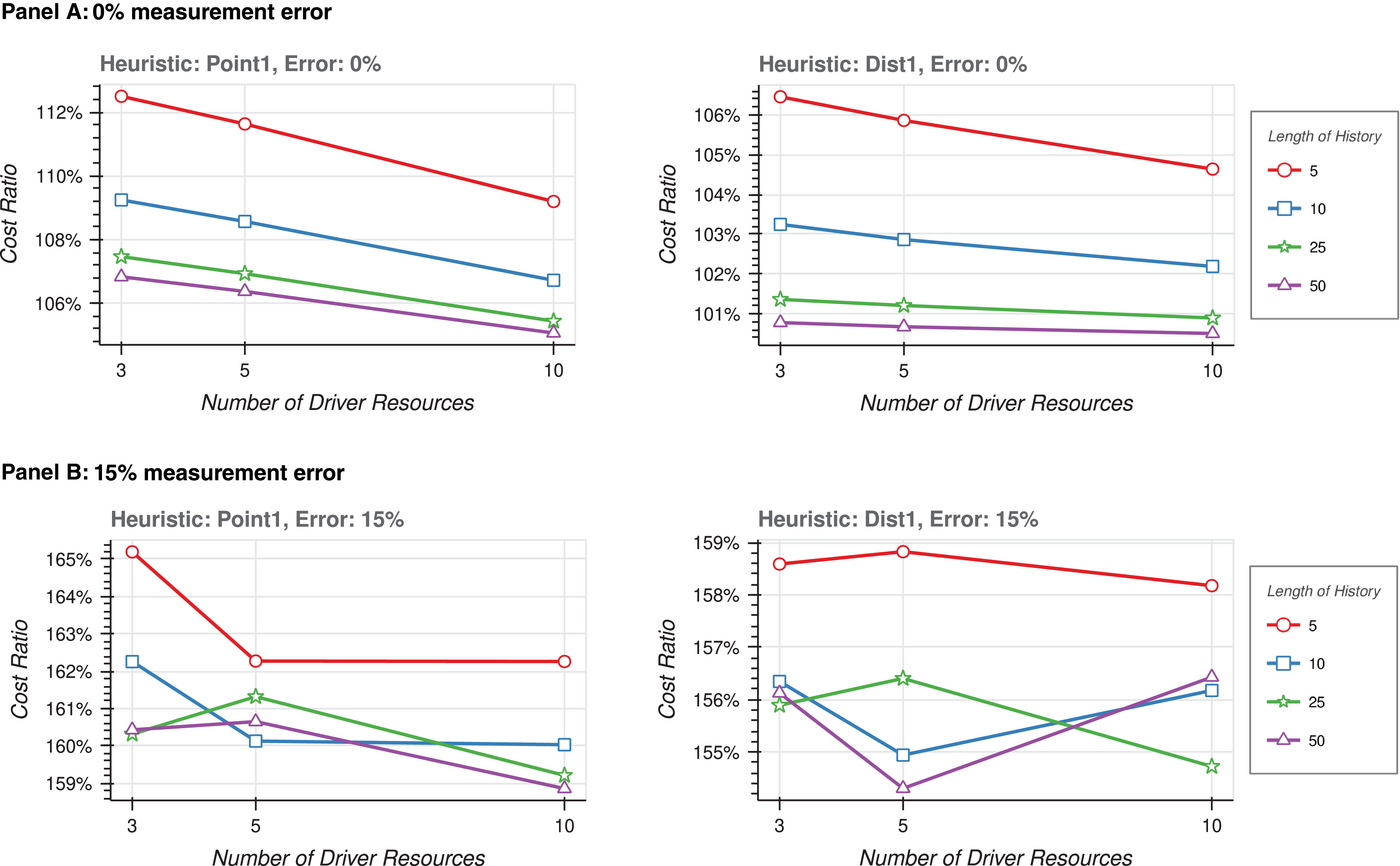
Interaction between measurement error, length of history, and number of driver resources. Cost ratio as a function of the length of history and number of driver resources for the Point1 and Dist1 heuristics. Panel A (B) shows results for low (high) measurement error. See Figure 1 for definitions of terms and description of the method. Each data point has 1000 observations.

Together, we conclude that measurement error reduces and could even reverse any gain due to the number of drivers or the precision in the ratios that relate the usage among driver to non‐driver resources. The intuition is that measurement error affects the installed capacity for both the driver and the non‐driver resources and that as we increase the number of driver resources, the magnitude of the problem (relating to non‐driver resources) decreases. The data suggest that the increased error in the installed capacity of driver resources overwhelms the marginal gain due to the reduction in the number of non‐driver resources or gains in determining their installed capacities. The implication is that in settings with high measurement error, firms need to be judicious in implementing partial improvements of their data collection processes, particularly when they employ sophisticated heuristics to fill in for limited information.

Finding 4: Partial improvements in precision or in the number of drivers can worsen system performance, particularly in settings with high measurement error. This finding is obtained because increasing the number of driver resources might also increase the associated measurement error.

ROBUSTNESS CHECKS

See Section A5 in the Online Appendix for additional details on each of these sensitivity tests.

Choosing driver resources

The centrality of driver resources implies that how we choose the set of driver resources matters. We have used the largest total cost method, the “Willie Sutton” rule, ¹⁷ which is consistent with practice. We consider four alternatives to this greedy algorithm: random choice, resources most used by products, maximum average absolute correlation with other resources, and stepwise regressions.

We find that the greedy algorithm yields the best results because this approach reduces the total costs of non‐driver resources (see Figure A7). This finding holds with positive measurement error and for the other heuristics. These results echo extant results in the operation management literature; for example, Bassok et al. (1999) and Biller et al. (2005) show that greedy algorithms are effective means for making pricing and production decisions.

Finding 5: How firms choose driver resources matters because of their central role in capacity planning. We find that a greedy algorithm for choosing the most expensive resources does best relative to methods that focus on maximizing information content.

Method for assigning resources to cost pools

Results thus far employ the NFL method to assign resources to drivers: cost pools take turns. In each turn, the cost pool chooses from the remaining unassigned non‐drivers resources the one with the highest correlation. We examined two alternate methods to assign non‐driver resources to drivers (i.e., to form cost pools): random assignment and a correlation‐based assignment. The random method is self‐explanatory. Under the correlation‐based method, we assign each non‐driver resource to the driver with the highest correlation in usage (based on the firm's production history). Note that these procedures produce an imbalanced (in terms of the number of resources and their cumulative value) cost pools. Inferences from these two alternate methods mirror those reported here. We conclude that the method for forming cost pools is not critical in capacity planning. This finding echoes findings in the research that examined the same question in the context of cost system design (Balakrishnan et al., 2011).

Picking the second driver for triangulation

The main results are from choosing as the second driver for the Point2 and Dist2 heuristics the available driver with the highest correlation. As an alternative, we estimated a stepwise regression with all remaining drivers and used the Akaike Information Criterion to select the second driver with the greatest explanatory power. Our inferences regarding the value of triangulation continue to hold. We conclude that simple methods to select the second driver suffice from the perspectives of generalizability and ease of implementation.

Distribution of product demand

Our assumption that product demand distributions are normal facilitates closed‐form solutions for expected costs but is not central to our results. Normality of the resource demand distribution is reasonable because convoluting a reasonable number (20 products in our case) of any set of distributions tends to yield a normal distribution. See Section A.5.4 of the Online Appendix for additional details.

Variations in spot premium

Results reported thus far set the distribution of the spot premium as

$U(1.25,2.75)$

. We next explore the effects due to a change in the mean or the variance of this distribution. We expected the performance of a heuristic to degrade as the average spot premium increases because errors in capacity planning are costlier. However, as reported in Table A7, an increase in the mean premium improves the average cost ratio. Analysis reveals that the improvement is a function of the change in the denominator of the ratio overwhelming the change in the numerator. Specifically, the denominator of the cost ratio is from the full‐information solution. This value increases because a higher spot premium implies greater installed capacity.

Data in panel B of Table A7 show another intriguing pattern: The performance of the Point1 heuristic (but not the Dist1 heuristic) degrades as the variance in spot premium, across resources, increases. The intuition is that the variance in spot premiums does not affect the full‐information solution, as we plan the capacity for each resource on its own. However, this variance adversely impacts the performance of the Point1 heuristic. We use the solution for the driver (which uses the opportunity costs for that resource) to project the capacities for the non‐driver resources. An increase in the variance implies that there is a greater probability of a mismatch in the opportunity costs, and hence the stocking ratio in the newsvendor problem, of the driver and non‐driver resource pairs. That is, there is a greater error in the installed capacity for the non‐driver resource. The mismatch is moot with the Dist1 heuristic as it directly employs the known opportunity costs for the non‐driver resources when planning capacity levels. The implication is that refinements in the form of heuristics that include opportunity costs (e.g., Dist1) are particularly valuable in settings with “high” variance in spot premiums. ¹⁸

Finding 6: Variance in the opportunity costs of resources adversely affects the performance of ratio‐based heuristics. Triangulation is valuable in this setting, as is the use of heuristics that include information about opportunity costs.

CONCLUDING REMARKS

In this paper, we consider the efficacy of heuristics that permit firms to plan for capacity in anticipation of demand, when they have incomplete and imperfect information about resource demand. Results from numerical analyses suggest that easy to implement heuristics perform well in terms of their efficiency relative to a solution with full information. A simple system with a handful of driver resources that uses ratios to plan for all other resources delivers good performance. Moreover, easily implemented tweaks to these heuristics (e.g., using two drivers to “triangulate” rather than one as in traditional cost systems) lead to dramatic improvements. Finally, our data show that the firms may benefit the most from efforts at reducing the measurement error in the use of driver resources. These findings are robust to considerable variations in the underlying parameters.

Our insights can be extended in several ways. A step cost formulation is likely appropriate for some resources. In this case, we conjecture that the cost efficiency of the heuristics will improve because more demand observations map into the same resource capacity. In the limit, a resource whose capacity is independent of demand will be estimated with zero error in all settings. Of note, it seems important to consider resource flexibility, which alters the opportunity costs of advance purchases. For the same reason, considering firms with pricing power that alter realized demand is likely to be fruitful. As noted earlier, considering inventory policy is important for settings with seasonal demand. Finally, considering hard capacity constraints (so that excess demand is lost rather than met via spot purchases) is important as several industries have resources that impose hard constraints (e.g., there is limited potential for outsourcing an operating room).