To maintain future supplier competition, manufacturers may support financially distressed suppliers by sourcing from them, even if they are less efficient than competitors, and by procuring larger quantities from them at higher prices. We analyze these strategies in a model in which a manufacturer decides for one of two available suppliers, supplier bankruptcy risk is endogenous, and financial distress can lead to internal or external reorganization. Following bankruptcy, the remaining supplier may serve as a backup option. Our research identifies settings in which the manufacturer should support the distressed supplier. We also find that in some cases, a nondistressed supplier may charge price premiums due to its competitor's distress, while in other cases, it may use predatory pricing to drive its competitor into bankruptcy. We complement our results with a small case study and show how our model can explain patterns observed in industry.
The financial distress of suppliers is an important, and often expensive, source of supply chain risk (Ni et al., 2017; Yang et al., 2015). When, for example, a leading automotive interiors supplier, Collins & Aikman, entered bankruptcy, its customers suffered an estimated $665 million in damages (Barkholz & Sherefkin, 2007). General Motors alone incurred costs of more than $10.6 billion following the bankruptcy of its supplier Delphi (Simon & Cohen, 2008).
Bankrupt firms do not simply cease to exist. Typically, they file for Chapter 11 bankruptcy and seek to reorganize internally (Iverson, 2018; Yang et al., 2015), as demonstrated in the application for debt restructuring submitted by the automotive supplier Sanden Holdings (Tajitsu, 2020). This form of restructuring often includes pledging future profits (Tajitsu, 2020). Debtors also may grant debt relief if the outstanding debt is less than their expected costs for attorneys, accountants, and trustees during a bankruptcy process (Bris et al., 2006; Chutchian, 2020). If an internal reorganization fails, the bankrupt firm must reorganize its assets externally. A well‐known example is the case of US Airways, which filed for Chapter 11 bankruptcy in 2013 and then merged with its direct competitor American Airlines (Harlan, 2015). Similarly, during the reorganization of the automotive supplier Visteon, its direct competitor Johnson Controls Inc. sought to strengthen its own market position by acquiring Visteon's assets (Brickley & Stynes, 2010). These types of consolidations in supply markets tend to result in price increases. In the Collins & Aikman bankruptcy, for example, customers such as General Motors, Ford, and Fiat Chrysler Automobiles experienced a rise in sourcing costs of $325 million (Barkholz & Sherefkin, 2007).
To mitigate losses from price increases and supply shortages and to potentially benefit from synergies due to vertical integration, some buyers acquire the assets of their bankrupt suppliers themselves rather than relinquishing them to remaining suppliers (Aïd et al., 2011; Lienert, 2016; Novak & Eppinger, 2001). When General Motors' supplier Clark‐Cutler‐McDermott went bankrupt, the potential supply shortage threatened the shutdown of multiple General Motors plants, with possible losses of several million dollars (Lienert, 2016). To avoid these losses, General Motors acquired the necessary assets from Clark‐Cutler‐McDermott (Gleason, 2016; Lienert, 2016). This case is a classic example of backward integration, a strategy that firms may choose to reduce supply‐side uncertainty and costs (Lin et al., 2014; MacMillan et al., 1986). However, as with any technological transfer—whether involving horizontal or vertical integration—the integrating firm faces additional costs, including those due to asset and knowledge transfer effort (Galbraith, 1990; Lukas et al., 2012). In addition, long before such an acquisition, it is uncertain which firm will acquire the assets: A competitor might expect smaller absorption costs and thus bid more aggressively.
Besides such reactive measures, supply chain risk management generally suggests the taking of proactive action (Augustine, 1995). Whether a supplier eventually files for bankruptcy depends on various factors. Proactive manufacturers can leverage different measures to predict the probability and intensity of such an event and act accordingly, even without absolute certainty. As Blome and Schoenherr (2011) and Moules (2012) note, proactive manufacturers often carefully monitor their suppliers' financial situations. Indicators such as the Altman Z‐score and credit default swaps can be valuable sources of financial distress information when available (Blome & Schoenherr, 2011; Simkovic & Kaminetzky, 2011). Additionally, firms can use global risk indicators to evaluate suppliers' risks based on their geography, operational performance measures, or historical information from previous shocks that have affected suppliers, and thereby estimate the exposure of suppliers to shocks (Amarnath et al., 2021; Blackhurst et al., 2008; Nyimbili et al., 2018; Tang, 2006).
When buying firms expect adverse cash flow shocks to hit their suppliers, they can act to reduce potential negative impacts (Blome & Schoenherr, 2011; Swinney & Netessine, 2009; Wu, 2017). In a series of interviews, multiple supply chain managers of large manufacturers in the automotive and electronics industries revealed that they sometimes support financially distressed suppliers by providing them with more business to maintain a competitive supply chain in the long run (Blome & Schoenherr, 2011). Put simply, giving a distressed supplier business rather than withholding it increases the supplier's chance of survival. Of course, such supportive strategies are not without risk: Sourcing from a distressed supplier can lead to operational disruptions if the supplier files for bankruptcy despite the extra business. To counter the risks associated with selecting a less reliable supplier, manufacturers often have backup suppliers in place (Demirel et al., 2018; White, 2020).
The decision‐makers of large manufacturers thus face several important questions: Should they choose the seemingly low‐risk option by selecting a nondistressed supplier and thereby ensure smooth operations in the short term, or should they select the distressed supplier to strengthen its chances of survival and thus maintain sufficient levels of competition in the future? Under what circumstances should the decision‐makers select the distressed supplier? Should they operate with backup suppliers? Addressing these questions requires a consideration of the endogenous bankruptcy risks that affect competition between suppliers and, in turn, the manufacturer's sourcing and suppliers' pricing decisions.
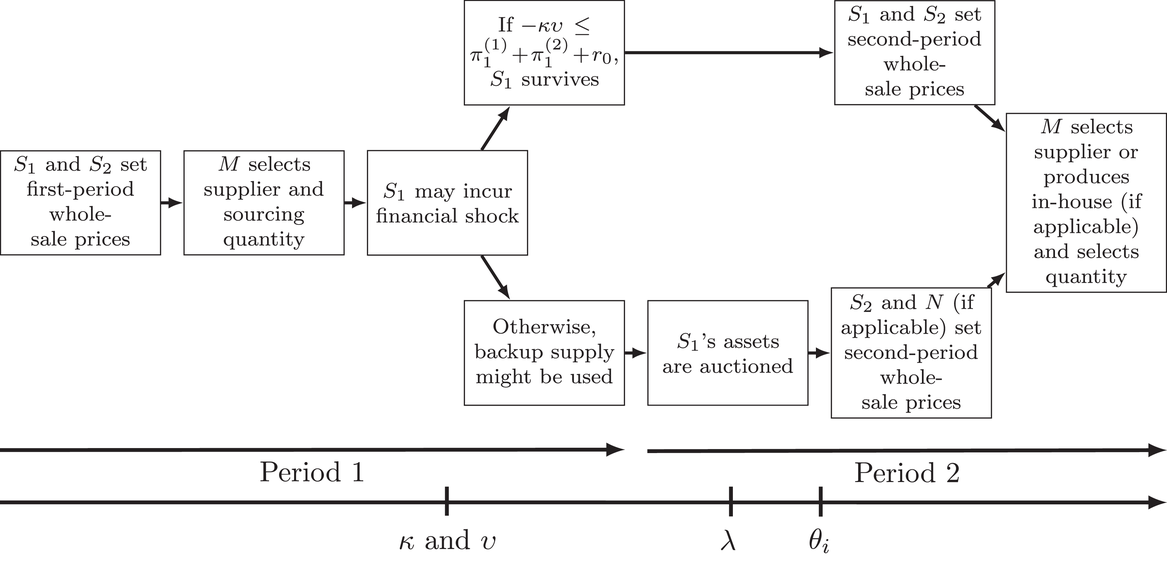
To provide structural insights into these questions, we model a game with two periods. In the first period, a manufacturer faces two suppliers, one of which is in financial distress. Considering both suppliers' wholesale‐price quotes, the manufacturer selects one supplier for this period; that is, the manufacturer cannot use a dual‐sourcing strategy. Then, with some probability, one supplier is hit by a random financial shock. Depending on the outcomes of the endogenous pricing and sourcing decisions, this shock may lead to the distressed supplier's bankruptcy. In the case of bankruptcy, this supplier may try to reorganize internally, pledging future profits and asking for debt relief from creditors. If this effort succeeds, the supplier continues its operations and the manufacturer receives its full order. If this effort fails, the manufacturer will not receive its order from the bankrupt supplier, so it must reach out to the remaining supplier, which offers the products at an updated, monopolistic price. The manufacturer sells any delivered products at a quantity‐dependent market‐clearing price. Next, the bankrupt supplier's assets are sold in an auction, where the remaining supplier, the manufacturer, and an outsider can bid; the latter may aspire to enter the business as a new supplier. The auction's winner then pays its bid and incurs stochastic absorption costs, which include the transfer and setup of the assets, among other costs. While the firms only have a rough idea about the distribution of each firm's absorption costs before the bankruptcy, they will receive additional information during the auction phase, leading to more accurate estimates of their absorption costs. In the second period, depending on the outcome of the first period, the manufacturer can source from one of two competing suppliers, procure from the sole remaining supplier, or produce in‐house. Considering strategic, forward‐looking firms, we analyze their equilibrium pricing and sourcing strategies.
The results of our game‐theoretic analysis demonstrate that financial distress in the supply base has important implications for the supplier selection decision. Basing such decisions solely on immediate purchasing costs or on costs directly associated with the bankruptcy of a supplier can have substantial negative financial consequences. Instead, the manufacturer should also consider the long‐term consequences of its supplier's possible bankruptcy. We find that the suppliers' production costs are a critical factor for the manufacturer in determining whether and to what extent to support the distressed supplier. If the distressed supplier has relatively high production costs compared to the nondistressed supplier, the former plays only a marginal role in ensuring effective competition, and the manufacturer has no incentive to support it. If the production cost disadvantage is less severe, however, the manufacturer might select the distressed supplier despite this disadvantage. In addition, the manufacturer may increase its sourcing quantity and be willing to pay more to this supplier. These effects persist if the distressed supplier has a slight production cost advantage.
Noting this pattern, we identify three important boundary conditions on the manufacturer's support. First, if the probability that a shock will occur is small, then there is no reason for the manufacturer to change its sourcing strategy. Second, suppose the probability of a shock is high and its intensity so severe that even generous support could not substantially improve the supplier's survival chances. In that case, forgoing this supplier is the manufacturer's best option. The third boundary condition relates to situations in which the supplier faces financial distress despite a production cost advantage (e.g., because other business divisions of the firm are struggling); in this case, the manufacturer decreases its support.
The financial distress of a competitor may allow a nondistressed supplier to increase its prices—after all, it is desirable for the manufacturer to choose a reliable supplier in the first place—but we also observe mechanisms that drive the nondistressed supplier to reduce its prices. On the one hand, reducing prices might be necessary to be selected as the primary supplier because the manufacturer would otherwise prefer to support the distressed supplier. On the other hand, competitive (sometimes even predatory) price reductions by the nondistressed supplier could decrease the distressed supplier's margin, increase its bankruptcy risk, and elevate the nondistressed supplier's chances to serve as a backup supplier.
Finally, based on interviews within a multiple case study of three manufacturing firms, we find that each of these firms actively engages in supporting distressed suppliers in their selection process (see the Supporting Information). Consistent with our model, they seek backup supply to limit potential damages. Uncertainty of asset auction outcomes often motivates these firms to find solutions before bankruptcy, and acquiring a bankrupt firm's assets is seen as a last resort. The managers of the case‐study firms indicate that suppliers seek to leverage the financial distress of their competitors by adjusting their prices strategically, which is consistent with our results.
LITERATURE REVIEW
Sourcing decisions that include distressed suppliers have been widely analyzed in the supply chain risk management literature (Babich et al., 2007; Demirel et al., 2018; Kazaz & Webster, 2015; Kouvelis & Li, 2008; Mendelson & Tunca, 2007; Tomlin, 2006). For example, Tomlin (2006) and Babich et al. (2007) analyze various risk‐mitigation strategies, such as inventory carrying, utilizing multiple suppliers, and passive acceptance. Kouvelis and Li (2008) and Demirel et al. (2018) focus on multisupplier strategies, such as selecting one supplier as primary and the other as a backup. Demirel et al. (2018) find that the manufacturer is typically worse off when a backup supplier exists. These studies treat supplier default risk as exogenous, such that whether a buyer sources from a distressed supplier has no impact on its survival probability. Qualitative studies complement these findings by allowing default risk to be endogenous and affected by the buyer's decision (Blome & Schoenherr, 2011; Spekman & Davis, 2004). Blome and Schoenherr (2011) also report cases in which a buyer deliberately sources from a financially distressed supplier to maintain long‐term competition, a strategy that often involves paying higher markups (Spekman & Davis, 2004). We seek to bridge the gap between studies that apply analytical models with exogenous supplier default risk to examine supply chain risk management and qualitative studies that explicitly consider a buying firm's endogenous impact on supplier default risk.
Our investigation also relates to several studies at the finance and operations interface (Buzacott & Zhang, 2004; Dong et al., 2018; Dong & Tomlin, 2012; Popescu & Seshadri, 2013; Tanrısever et al., 2012; Wu, 2017). Whereas the implications of financial constraints or financial distress tend to be studied at the firm level (Boyabatlı et al., 2016; Iancu et al., 2017), some research also examines the supply chain level (Chod et al., 2019; Kouvelis & Zhao, 2012, 2017; Yang et al., 2012). Moreover, a particular stream of studies investigates trade finance instruments that might help a financially troubled firm (Babich, 2010; Kouvelis & Zhao, 2016; Li et al., 2016; Tang et al., 2017; Tunca & Zhu, 2018). Babich (2010) and Li et al. (2016) study collaborations between a manufacturer and a supplier in which one firm is able to support its troubled trade partner through upfront subsidies. Babich (2010) provides structural insights into the relationship of product characteristics, upfront subsidies, and the ordering and subsidy decisions of manufacturers. In situations in which financial instruments are not available, Tanrısever et al. (2012) show that a start‐up may sacrifice early profits to increase its survival chances; we similarly analyze situations in which upfront financial instruments are not applicable or already exhausted. Whereas Tanrısever et al. (2012) focus on the investment strategies of two competing firms, we examine the pricing strategies of one distressed and one nondistressed supplier, both competing for the same manufacturer's business.
Several studies offer evidence regarding financial distress and possible mitigation strategies in supply chains with three or more firms (Ellis et al., 2010; Swinney & Netessine, 2009; Wagner & Bode, 2008; Yang et al., 2015). Swinney and Netessine (2009) propose two potential strategies—short‐ and long‐term contracts—for a buyer dealing with two distressed suppliers, then compare the advantages and disadvantages of these strategies for a wholesale‐price‐setting buyer. When the supplier‐switching costs are low, the buyer prefers short‐term contracts. In a study quite closely related to ours, Yang et al. (2015) investigate one supplier that decides in each of two periods what wholesale prices to charge to two retailers, one of which is distressed. Assuming Chapter 11 bankruptcy reorganizations, Yang et al. (2015) compare different wholesale‐pricing schemes and their effects on the retailers' sourcing and pricing strategies. In our complementary analysis, we consider a supply chain in which one distressed and one nondistressed supplier compete for the business of a single manufacturer. In this distinct supply chain structure, production costs are more important drivers of agents' decisions than in Yang et al. (2015). We also consider absorption costs that arise when firms seek to integrate production assets. As a result, important dynamics arise that pertain to the context of our study but not theirs; in addition, not all of their structural findings apply to our setting. As an extension to Swinney and Netessine (2009) and Yang et al. (2015), we also consider a potential recourse in the form of a backup supplier, which might reduce the short‐term damages associated with bankruptcy, as well as the effects of a possible asset auction that could alter second‐period sourcing decisions.
Finally, our research builds on direct examinations of bankruptcies and other situations that may lead to a transfer of assets (Ahern & Harford, 2014; Brege, 2006; Bris et al., 2006; Cho, 2014; Farrell & Shapiro, 1990; Fee & Thomas, 2004; Lukas et al., 2012; Thorburn, 2000). When a U.S. firm fails to meet its payment obligations, it usually files for bankruptcy under Chapter 11 and tries to reorganize internally (Pulvino, 1999; Strömberg, 2000). To persist and reorganize its assets internally, the firm must make a convincing case that its future profits are sufficient to cover its current obligations. If it cannot do so and fails to negotiate debt relief, the bankrupt firm may try to sell its assets to the highest bidder (Thorburn, 2000). As shown by Galbraith (1990) and Lukas et al. (2012), who study mergers and acquisitions and technological transfers, taking new assets into operation involves additional absorption costs, such as those related to transportation, setup, and knowledge transfer. We use these features of bankruptcies and asset transfers to model the associated processes and costs. It is worth noting, however, that financial distress is not always a consequence of inefficient production. Other causes include recalls, lawsuits, customer payment delays, policy changes, unsuccessful investments, and economic downturns (du Jardin, 2016; Geng et al., 2015; Gordon, 1971; Mai et al., 2019).
MODEL
Consider a two‐period model. Manufacturer M sells a single product type on a supply‐elastic market at the end of each period. The products from the first period cannot be carried over to the second period. The products can be supplied by two suppliers, S1 and S2, with nonnegative per‐unit production costs c1 and c2, respectively. In our model, S1 is under financial distress, which means there is a positive probability that it files for bankruptcy, whereas this probability is negligibly small for S2; that is, S2 is nondistressed. Firms suffer financial distress for various reasons. Sometimes, they have inferior production technology and are noncompetitive (
). Others have weakly lower marginal costs (
), yet they also suffer from exogenous shocks such as injury claims, product recalls, or mismanagement (Scurria, 2020; Tajitsu & Shepardson, 2017). Our model captures both cases.
Following Swinney and Netessine (2009), we assume that S1 is seeking to stay in business and already uses all available external financing arrangements in the first period. All players in our model are risk‐neutral profit maximizers. However, we show and briefly discuss that even a distressed supplier that wants to minimize bankruptcy risk will pursue a profit‐maximizing strategy in our model (see Proposition 1). As a convention, we use superscript numbers in parentheses to refer to periods. Subscript
refers to the manufacturer, S1, S2, or a potential new entrant N, respectively. For ease of exposition and when the context is unambiguous, we drop the explicit reference to the period or player. We generally use the terms increase/decrease and higher/lower in a weak sense.
In the first period, each supplier quotes a first‐period wholesale price
; then, the manufacturer selects one supplier and chooses an order quantity
. This sequence is in line with the well‐studied and conventional price‐only approach, in which each supplier offers its unit price, and the manufacturer orders quantities based on these prices (Chen, 2012; Yang & Ma, 2017).
The manufacturer sells its products in the market. As in Tanrısever et al. (2012) and Yang et al. (2015), we assume that the realized market‐clearing price is decreasing in the offered quantity, specifically,
, with
. Our primary structural results remain if M is a newsvendor or a price setter selling to price‐sensitive customers. The manufacturer's profit in the first period, when it sources quantity
at wholesale price w(1), is
; the selected supplier
yields profit
; and the nonselected supplier
yields profit
. We assume
to avoid trivial cases in which sourcing from
cannot result in positive supply chain profit. Because we allow suppliers to charge prices above, at, or even below their per‐unit production costs, we can determine if and when predatory pricing might be optimal.
In addition to the profits generated in this focal supply chain, we assume that at the end of the first period, S1 may be exposed to an exogenous shock that affects its financial situation. Such shocks include natural disasters, fluctuations in raw material prices, or unsuccessful businesses outside the focal supply chain. For instance, during the COVID‐19 pandemic, some firms supplied the aviation industry among other industries. Those firms suffered significant revenue declines and became financially distressed, affecting their other lines of business. We assume that the shock does not directly affect the quantity that the supplier can produce; however, if the supplier has to file for bankruptcy in the aftermath of the shock and cannot be reorganized, it will not produce at all. For tractability, we consider S2 nondistressed so it will not be hit by a shock (put differently, even if a shock hits it, it would simply survive in our model). We assume that S1's financial shock has two random components. First, the random variable
captures the shock's occurrence. We denote the probability of occurrence (
) by k. Second, random variable
captures the shock's intensity. We denote its probability density function (p.d.f.) with
and the cumulative density function (c.d.f.) with
. While no one can predict bankruptcy with certainty, there are typically some rumors before such an event, and firms can use various methods to get a sense of the severity of such a shock on a supplier. Instruments such as credit default swaps, disaster risk indicators, and operational performance measures can go a long way in forming such estimates (Amarnath et al., 2021; Blackhurst et al., 2008; Simkovic & Kaminetzky, 2011). Accordingly, we assume k and
are public knowledge. These distributions essentially capture that firms could make rough estimates such as the following: “If the margin of a supplier is below 15% and the order volume is below $1,000,000, the supplier has a 50% survival chance.” Or, “If we withdraw our business, the supplier's bankruptcy chance is 80%.” The parameter k and the distribution
capture this intuition more formally. The distribution
is very general. It might even allow for realizations that are so negative—such as the litigation costs of airbag manufacturer Takata (Tajitsu & Shepardson, 2017)—that the supplier becomes bankrupt regardless of the manufacturer's action, at least in any equilibrium. In short, it is random whether a shock hits the supplier or not; and if it hits, how severe it is.
Similar to Swinney and Netessine (2009) and Yang et al. (2015), we assume that the distressed supplier files for bankruptcy if the sum of its first‐period profit and the financial shock is negative,
. Bankruptcies follow a structured process (Brege, 2006), and we assume Chapter 11 proceedings. If its future profits
are sufficient to cover the financing gap, S1 can pledge these profits to reorganize its assets internally and overcome its financial distress. As also observed in industry practice, we assume that the supplier turns to its creditors for debt relief r, which they grant if it prevents a costlier liquidation process (Hakim, 2005; Tajitsu, 2020). Specifically, if sufficient for reorganization, creditors grant a relief of up to
, where
is an exogenous threshold that captures the cost of liquidation for creditors. If the debt relief is sufficient to overcome an imminent bankruptcy, the supplier has successfully reorganized its assets internally. Upon successful internal reorganization, if the supplier is the selected supplier in period 1, it will deliver the ordered quantity q(1) at wholesale price
to the manufacturer. Regardless of whether S1 directly survives period 1 or does so due to an internal reorganization, we consider its distress to be overcome; it does not face any bankruptcy risk in period 2.
In contrast, upon failure of internal reorganization, if S1 has been selected as the supplier in the first period, there are no shipments from S1 to the manufacturer. In this case, S2 offers a wholesale price
, and the manufacturer decides to source quantity
from this firm (Gupta et al., 2021, make a similar assumption). This captures the idea of backup suppliers by Kouvelis and Li (2008) and Demirel et al. (2018). Whereas we consider backup supply, our model does not allow for dual sourcing by splitting orders.
The failure of the internal reorganization also leads to the next step in the bankruptcy proceedings, that is, S1's assets are sold to the highest bidder in a first‐price auction (Strömberg, 2000; Thorburn, 2000). Besides M and S2, which may submit bids
and
, respectively, we assume that outside parties seek to become new suppliers of M and may place bids, too. Without loss of generality, we capture outside parties as N, formally the third‐party firm with the highest willingness to pay for the assets. This firm may submit bid
. This approach is consistent with former work on bankruptcy proceedings (Ahern & Harford, 2014; Cho, 2014; Farrell & Shapiro, 1990).
In addition to paying the bid, the firm that wins the asset auction incurs absorption costs, comprising the costs of transferring, setting up, and integrating assets (Galbraith, 1990). The actual absorption costs
are only realized after the auction (some firms can be caught by surprise after an acquisition). At the beginning of the game, when firms make pricing and ordering decisions in the first period, they only know that the random variables
capturing the absorption costs are distributed with continuous p.d.f.s
on supports
, with
. After S1 becomes bankrupt and fails to reorganize internally, all firms obtain more information (e.g., as they learn more about the production assets). We capture the information‐updating through random variable Λ with support
, the realization of which all parties observe before the auction. We denote the p.d.f of Λ by
and the updated p.d.f. of
—after observing λ—with
. It holds that
.
If M or N acquire S1's assets, they can produce the product in the second period at a cost c1. If S2 acquires the assets, it can produce at cost
in the second period. If none of the firms finds it attractive to acquire S1's assets (e.g., due to high expected absorption costs), S1's assets are liquidated and are no longer relevant to the focal market. These effects pertaining to production costs apply if there are no synergies between a supplier's existing and potentially newly acquired assets, as is often the case in the automotive industry, where each manufacturer has specific requirements, and production requires specific tooling (Lienert, 2016).
In the second period, the manufacturer asks the remaining supplier(s) to quote the second‐period wholesale price(s)
,
. If the manufacturer acquired S1's assets, it can source the product from S2 or produce in‐house at cost c1. Again, the manufacturer sells quantity q(2) at the market‐clearing price
. Second‐period profits
,
,
, and
, if applicable, are derived similarly as in the first period, except that the manufacturer can produce in‐house at cost c1 if it acquired S1's assets; S2's production cost would be
if it acquired S1's assets; and N's production cost would be c1 if it acquired S1's assets. We present an overview of the game in Figure 1.
Game sequence and timing of the random variables' realizations.
In our analysis, we focus on trembling‐hand equilibria (Selten, 1975), which is a refinement of the Nash equilibrium and accounts for potential but unlikely deviations from the equilibrium strategies. For ease of exposition and without changing any structural insights, we assume that whenever M bids the same as S2 or N, then M wins the auction, and whenever S2 bids the same as N and higher than M, then S2 wins the auction. Likewise, without loss of generality, we assume that if both suppliers' wholesale prices yield the manufacturer the same expected profit, M sources from S1 if and only if doing so strictly decreases this supplier's bankruptcy risks.
ANALYSIS
Using backward induction, we first analyze second‐period strategies (Section 4.1). On the basis of the outcomes for different scenarios (survival yes/no, internal reorganization yes/no, assets acquired by M/S2/N or liquidated), we then move to the first period to study the pricing and sourcing strategies (Section 4.2). Next, we analyze the impact of financial distress on strategies and profits (Section 4.3). Finally, we discuss the value of having access to a backup supply option (Section 4.4).
Second‐period strategies
An important concept for our analysis is the hypothetical wholesale price that suppliers would charge if they were monopolists; this monopolistic wholesale price also serves as the upper limit in competitive settings. (All proofs can be found in the Supporting Information.)
Suppose there is only one supplier, i, which acts as a monopolist. This firm charges the wholesale price
in equilibrium.
Building on this lemma, we can analyze the second‐period pricing decisions in competitive settings. Let
denote M's sourcing costs if firm
owns S1's assets, where
indicates that no firm acquired the assets. The exact functional forms of
follow directly from the next theorem. We use
,
,
,
, and
to denote equilibrium wholesale prices, equilibrium sourcing costs, equilibrium sourcing quantities, equilibrium bids, and expected equilibrium profits of firm i, respectively.
In the unique second‐period equilibrium,
if S1 survives,
if
, then
sets
and
sets
, with
and
,
otherwise, S1 and S2 set
;
if M acquired S1's assets,
if
, then S2 sets
,
otherwise, S2 sets
;
if S2 acquired S1's assets, then S2 sets
;
if N acquired S1's assets,
if
, then firm i sets
and firm j sets
, with
and
,
otherwise, S2 and N set
;
if no firm acquired S1's assets in the asset auction, then S2 sets
;
is the cheapest option among the wholesale prices presented in (a)–(e) and the potential in‐house production costs c1 (in case M acquired the assets);
M sources
.
In the second period, firms are nondistressed, so M sources the optimal Cournot quantity
from the cheapest option, which follows from parts (f) and (g). The pricing strategies in parts (a) and (d) then are a direct consequence: If S1 survives or N has acquired S1's assets, the two suppliers try everything in their power to be selected. Specifically, if cost structures are similar enough (
and
), the supplier with higher costs offers a price equal to its production costs, and the other supplier bids slightly less (technically, it bids some
less). If supplier i has a substantial production cost advantage with
, then it sets its price to the monopolistic level
and still is selected. In part (b), M has acquired S1's assets and S2 offers a wholesale price below M's production costs, if profitable. If c1 is very large, S2 asks for the monopolistic price
. A higher price could still lead to selection, but it would adversely impact the quantity and thus S2's profit. If
, S2 sets
. Parts (c) and (e) characterize the aftermath of S2's asset acquisition and the asset liquidation, respectively. Both allow S2 to charge monopolistic prices that only depend on S2's production costs.
Suppose S1 files for bankruptcy and cannot reorganize internally.
Let
be the bid of firm
in equilibrium and
.
Let
map the quadruple of bids to the winner i of an auction, where ∅ denotes the case in which no firm acquires the assets.
That is,
is the winner of the auction.
Let
for
.
There exist multiple equilibria in the asset auction. All equilibria have the same winner and the same winning bid.
is a partition of
.
If
and
, then
.
If
and
, then
.
There exists a nonempty subset
such that
if
, then
⇔
;
if
, then
; and
if
for any
, then
.
If
, there exists a nonempty set
such that
if
, then
;
if
, then
; and
.
If
, then
and
.
This theorem proves the existence of a unique winning bid and unique winner in the auction. If multiple firms submit the highest bid, as a tiebreaker, the manufacturer wins the auction if it is among the highest bidding firms, and S2 wins otherwise (which follows from our assumptions in Section 3). We see that it is possible to partition the support of λ into four sets
,
, such that
indicates that firm i wins the auction.
Theorem 2 has several important implications. Firms M, S2, and N can all benefit from buying the assets if their expected absorption costs are small: M could not only obtain the distressed firm's margin and maintain future competition but could also remove double marginalization; S2 could become a monopolist with strong pricing power; and N could enter a new business rather than choosing the outside option of zero profit. Part (b) states that M's incentives are the strongest unless it faces a significant absorption cost disadvantage. In that case, part (c) states that S2 has more substantial incentives than N, unless S2 itself is at a sufficiently pronounced absorption cost disadvantage. Thus, expected absorption cost differentials could be a vital determinant of the outcomes in some of our motivating examples, where either the manufacturer (e.g., GM) or the competitor (e.g., Johnson Controls, Inc.) made the highest bid (Brickley & Stynes, 2010; Gleason, 2016).
Part (d) provides insight on M's second‐period profit
. By definition,
is the second‐period equilibrium profit that would be reached if S1 stayed in business. For
and specific tuples of absorption costs, M could improve its second‐period profit in the case of S1's bankruptcy. That is, if S1 were in distress for reasons other than production inefficiencies and M acquired S1's assets, the manufacturer could benefit from S1's bankruptcy and the failure of the ensuing internal reorganization because this scenario removes double marginalization. However, for
, this can never happen, and S1's bankruptcy always leads to reduced profit for M, even when M acquires S1's assets.
Part (f) states that if S2 has a substantial production costs advantage (
), it cannot benefit from S1's bankruptcy. In all other cases (part e), S2 benefits from its competitor's bankruptcy whenever S2 acquires S1's assets at a low cost—enabling S2 to charge monopoly prices—and when
is small enough compared to
and
(see the proof of Theorem 2 for a formal derivation of this observation). Like M, S2 may benefit from its competitor's bankruptcy even if N has zero absorption costs.
The results obtained from Theorem 2 facilitate the derivation of the following insights regarding the manufacturer's optimal ordering decision and the resulting market‐clearing price, which also indicates the effects of a supplier bankruptcy on M's customers in the second period.
Assume that S1 filed for bankruptcy and failed to reorganize internally.
If
, then (i)
and (ii)
.
If
, then (i)
and (ii)
.
If
, then
.
Additionally,
.
We see that S1's bankruptcy may either improve or reduce consumer welfare. Technically, whenever
and
, consumers buy more products at lower prices, which corresponds to an increase in consumer welfare. If the manufacturer acquires S1's assets, equilibrium sourcing costs will never increase (part a.i). If the acquired assets are more efficient than those of S2, equilibrium sourcing costs are strictly smaller than they would have been if S1 had stayed in business (part a.ii). Consequently, the equilibrium quantity increases, and the market price decreases. However, if either S2 or no firm acquires the assets, and S2 has not been at a strong production cost advantage, then the equilibrium wholesale prices are larger than in the hypothetical case of S1's survival (part b). The equilibrium quantity then decreases, and the market price increases. The entry of a new player leads to the same outcomes as the survival of S1 would have (part c).
First‐period strategies
In the first period, M selects
,
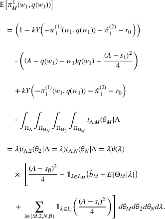
, leading to an expected profit of
. If M selects S1, S1's bankruptcy probability is
. In the case of bankruptcy, the manufacturer makes profit
from utilizing the now monopolistic S2 as a backup supplier (for the derivation of this technical result, see Lemma 3 in the Supporting Information). If M acquires the assets, M incurs the bid price and absorption costs. Depending on whether and which firm
will own the assets in the second period, the manufacturer has second‐period profits of
. All together, we have
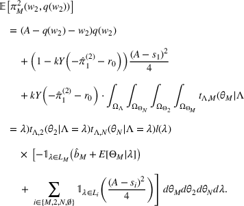
If M sources from S2 in the first period, the bankruptcy probability becomes
, and no backup supply is needed, so
The optimal first‐period order quantity when selecting
as the primary supplier at wholesale price
is
. This information is known to each supplier, so each can calculate its competitor's first‐period wholesale price that would maximize M's expected profit. Yet, S2 may also generate profit as a backup supplier. Thus, when it decides on the optimal first‐period price, S2 does not focus exclusively on the consequences of being selected; instead, even in cases in which it will not be selected, it may strategically opt for a lower wholesale price to increase the pressure on its competitor and thus its chances of acting as a backup supplier.
Whereas optimal second‐period strategies can be expressed in closed form, there are generally no closed‐form expressions of the manufacturer's and suppliers' equilibrium pricing strategies in the first period. Denoting the equilibrium quantity that M sources from
at prices
with
, the following result proves the existence of a unique equilibrium:
In the first period, there exists a unique subgame‐perfect equilibrium
,
,
,
,
,
. If S1 can make an offer leading to its selection, it does so in equilibrium. If S2 can make an offer leading to its selection, it does so in equilibrium unless serving as a backup supplier leads to higher expected profits.
This theorem provides insights into three strategic outcomes. S1 always follows the same strategy, which is to attempt to make the winning offer. S2's strategy is more interesting in that it may seek to make the winning offer but may also purposefully make the second‐best offer, even if it could price to win. Forgoing becoming the primary supplier is attractive for S2 if potential monopolistic pricing as a backup supplier is very profitable (i.e., if c2 is small).
Having established the existence of the unique first‐period equilibrium, we next offer three propositions to characterize optimal strategies in terms of pricing, quantities, and profits. From here on, we let
denote the set of tuples
.
In any equilibrium, it holds that
and
;
if
, then
;
if M selects S2 as the primary supplier, then
; if M selects S1 as the primary supplier but benefits in the aftermath of S1's bankruptcy, then
; and
there exists
such that
.
To maximize its total profit, S1 prefers survival to bankruptcy; survival retains the potential to generate positive profit in the second period. Maximizing first‐period profit implies minimizing bankruptcy risk, so S1 would never offer bids below its production costs (part a). In part (b), we show that a substantial production cost advantage for S2, specifically
, is a sufficient condition for charging a wholesale price above its marginal costs, irrespective of the potential for asset acquisitions in the aftermath of bankruptcy; if this substantial advantage does not exist, S2 might charge at the level of its production costs or even below that, as we examine in Section 4.3. Complementing this consideration, part (c) implies that M typically charges its customers a price above the wholesale price, as one would surmise. However, extreme situations exist where M would charge below its marginal costs, as seen in part (d). This can only arise if M materially benefits from S1's survival and combines paying a high wholesale price and keeping its prices low to attract more demand. (Whether pricing below costs is permissible in this case is outside the scope of our analysis.)
The following two propositions reveal insights into the complex strategic trade‐offs involved in the first‐period decision making and their interaction with the first and second moments of M's and S2's absorption costs,
and Θ2, respectively.
denotes the prior expectation, which is
.
There exist nonempty subsets
,
, such that
if and only if
, then
and
decrease in
, whereas
increases in
, and
increases in
;
if and only if
, then
and
increase in
, whereas
decreases in
, and
decreases in
;
if and only if
, then
and
increase in
, whereas
decreases in
, and
decreases in
;
if and only if
, then
and
decrease in
, whereas
increases in
, and
increases in
.
Part (a) is partially intuitive. For cases with
, more considerable absorption costs for the manufacturer imply that the manufacturer is worse off in expectations. At the same time, S1 fares better since the manufacturer must be more supportive (part a.ii). That, in turn, comes at the expense of S2, whose profit also decreases in expectation.
This mechanism does not have to be prevalent, however. Part (b) states the existence of cases,
, in which the relationships in part (a)(i) reverse. Part (b)(ii) provides the missing link between the expected profit functions and the expected absorption costs of the manufacturer. Suppose
where S2 has a sufficiently high probability of purchasing the assets of S1 in the case of bankruptcy. Then, an increase of M's absorption costs implies that, in equilibrium, S2 can win the asset auction with a smaller bid, making the acquisition more interesting. In anticipation, S2 decreases its first‐period wholesale price to increase the pressure on S1. Therefore, S2 is better off. In expectation, the overall effect is so strong that even the manufacturer benefits, whereas S1 suffers.
Part (c) is analogous to part (a) but examines the effects of S2's expected absorption costs. The manufacturer benefits from increases in S2's absorption costs for
because it is more likely to acquire S1's assets at a lower price. Therefore, it is willing to reduce its support for S1 in the first period, increasing the likelihood for S2 to serve as a backup supplier, which raises S2's expected profit. That all happens at S1's expense, as it receives less support and is more likely to become bankrupt. Finally, part (d) is analogous to part (b).
Whereas our intuition regarding the role of expected costs suggests that they affect expected profits (as shown by Proposition 2), the impact of uncertainty, here expressed in the variance of absorption costs,
, is more complicated. The following result provides some insights. Let
denote the prior variance (i.e., before the realization of λ).
There exist nonempty subsets
,
, such that
if and only if
, then
and
decrease in
, whereas
increases in
, and
increases in
;
if and only if
, then
and
increase in
, whereas
decreases in
, and
decreases in
;
if and only if
, then
and
decrease in
, whereas
increases in
, and
increases in
; and
if and only if
, then
and
increase in
, whereas
decreases in
, and
decreases in
.
Keeping the expected absorption costs prior to updating (
) fixed, the absorption cost variance can have an impact only if the payoff functions are asymmetric. While Proposition 3 holds for general functional dependencies, we use—for expositional clarity—two special cases to discuss the emergence of these asymmetries. Suppose, in (a) and (b),
linearly increases in λ, and
for
is independent of λ. Similarly, in (c) and (d), suppose
linearly increases in λ, and
for
is independent of λ.
Consider
in part (a). For such an
, S2 tends to have a relatively high probability of acquiring S1's assets in an auction. If the realization of λ clearly exceeds its expected value,
becomes meaningless because either M will not place a positive bid in the first place or the outside bidder N already bids more than M. Therefore, for any realizations of λ above a given threshold, λ will not affect S2's profit function. However, if the realization of λ is sufficiently far below its expected value, it affects S2, as M can make more competitive bids, effectively forcing S2 to bid more. Due to this asymmetry, S2's profit decreases in
. In turn, S2 will find the acquisition of assets less profitable in expectation and will thus bid less aggressively in the first period (statement a.ii), which reduces the expected profit for M. This effect dominates other effects for M such that M also suffers from an increase in
. S1 alone benefits, as it faces less competition in the first period and thus is more likely to survive.
Part (b) captures the settings,
, in which the impact of
reverses. For these
, it is likely M that would acquire the assets. If the realization of λ clearly exceeds its expected value, the loss will be limited. Eventually, M will not place a positive bid but rather relinquish the assets to S2 or N. In contrast, if the realization of λ clearly falls short of its expected value, then M still acquires the assets but at a much smaller cost. This induced asymmetry causes M to benefit, in expectation, from higher variance in its absorption costs. Consequently, M is less concerned about bankruptcy and decreases its support, as statement (ii) expresses. In turn, S2 benefits because the likelihood of becoming a backup supplier increases. Only S1 suffers. Parts (c) and (d) follow a similar logic concerning
.
Impact of financial distress on optimal strategies
We next take a more nuanced approach to evaluate the impact of financial distress on sourcing, quantity, and pricing decisions to characterize better how and when the manufacturer might be able and willing to support S1. The following analysis also sheds light on the aggressiveness of S2, progressing from monopolistic pricing to competitive pricing, and finally to predatory pricing. To characterize the impact of financial distress, let
and
denote the equilibrium wholesale prices in the benchmark setting in which S1 is not financially distressed (i.e., S1 survives period 1 with certainty, regardless of M's decisions). Let
denote the optimal sourcing strategy in the same setting. Then,
corresponds to the benchmark equilibrium in which S1 is nondistressed. To distinguish the effects on the order quantity that arise because both suppliers take financial distress into account (i.e.,
vs.
) from the effects that arise because M takes financial distress into account (i.e.,
vs.
), we also capture the theoretical value of
, which is M's best response to the wholesale prices arising in the scenario without distress. Although this is not an equilibrium outcome, it facilitates interpretation as it manifests an important benchmark.
Let
denote the set of all feasible tuples
.
If
, then
and
.
There exist
and
such that if
or
and
, then
, for
and
.
There exist
,
,
,
, and
such that if
,
,
, and
, then
.
There exist
,
, and
such that if
and
, then
; and
, then
.
There exist
and
such that if
,
, and
, then
, and if and only if S1 is nondistressed, M sources from S1.
The tuple sets can be characterized as follows:
If
and
, then
.
If
,
, and
, then
.
The first five parts of Proposition 4 capture different competitive environments, and the last part characterizes the most critical parameter sets.
In part (a), S1 is at a production cost disadvantage. Without financial distress, S1 would not be selected in equilibrium. However, if S1 is financially distressed and the offered wholesale prices are unchanged, then M might select and support S1, which means M increases its sourcing quantity from this supplier. This strategy resonates with real‐world observations of some automotive and electronics manufacturers that purposefully and explicitly source from suppliers to support them (Blome & Schoenherr, 2011). S1 can exploit this strategy and charge a higher wholesale price. For S2, the impact of financial distress can go either way. If it makes S1 more competitive (i.e., if the manufacturer is willing to pay a surcharge), S2 offers a reduced wholesale price. However, if S1 becomes less competitive due to the risk of M facing a monopolistic backup supplier in the case of a bankruptcy, S2 may increase its wholesale price to a level between the competitive baseline (
) and the monopolistic price (
).
Part (b) highlights that neither M nor S2 changes their strategies compared to a nondistressed situation if the exogenous shock is sufficiently unlikely, that is, with a probability below a threshold k1. While the first condition allows k1 to be zero, we explicitly state in the second part that even strictly positive probabilities may not affect any strategies. This latter situation arises when the potential damages of a shock for S1 are sufficiently low.
Part (c) focuses on situations where sourcing from S2 in the first period leads to a high bankruptcy probability, while S1 has a limited production cost advantage. If the intensity of the shock is small—that is, if a bit of support would have substantial effects (specifically,
)—the manufacturer increases its order quantity to support S1.
Part (d) characterizes the strategies when S1's assets are even more efficient, as indicated by the parameter set
in part (f.ii). If M anticipates acquiring the assets in the case of bankruptcy (see part d.i), support from M may turn into added pressure, expressed in the form of reduced sourcing quantities from S1. However, if S2 were to acquire S1's assets, S2 would engage in competitive pricing, and at times even predatory pricing, being willing to charge a wholesale price strictly below its marginal costs.
Part (e) sheds light on cases in which S1 has a substantial production cost advantage and both the probability and intensity of the shock are large. In these cases, even if M selected S1 in the first period, S1 would still face a high risk of becoming bankrupt; consequently, M then avoids sourcing from S1. That reflects the strategy of sourcing from a healthy supplier in the first place. When this happens, S2 may demand surcharges in anticipation of being preferred. These motives differ from those that apply under the conditions in part (d), where M reduces the sourcing quantity in anticipation of eventually acquiring S1's assets. In part (e), this condition is not present. Here, the key motive is that supporting S1 is relatively expensive, given the high intensity of the shock (specifically,
).
We next examine the impact of financial distress on the expected profits of the different firms, comparing them against a hypothetical profit that could be realized if S1 was nondistressed.
Let
denote expected profit for firm
minus the hypothetical profit for firm i if S1 were not under financial distress.
If
,
then
and
;
there exists
such that
, and there exists
such that
; and
there exists
such that
, and there exists
such that
.
If
,
then
,
, and
; and
there exists
such that
; and there exists
such that
.
If
,
for all
.
There exists
such that
for
.
This proposition does not pose any restriction on the prior absorption cost variances
,
. However, to form an intuition, it is insightful to consider a thought experiment. Suppose the absorption costs were fairly predictable with sufficiently low variances. Then, all firms can predict, with high confidence, who would win a potential asset auction.
Part (a) characterizes settings in which S1 has more efficient assets than S2 (
). In those cases, neither S2 nor any outside firm would be considered in the first period or could become a second‐period supplier if S1 was nondistressed; therefore, neither S2 nor N are worse off in expectation due to financial distress. For M and S1, the effects of financial distress can go either way, but they tend to move in opposite directions. If M's absorption costs are sufficiently low, M might benefit from distress due to the higher likelihood of acquiring efficient production assets. As M's absorption costs increase, its expected profit declines, and it might become worse off under financial distress. However, as M's absorption costs increase further, all else held equal, acquiring the assets becomes relatively cheaper and more likely for S2. In anticipation of this, S2 then prices more aggressively in the first period, to the overall advantage of M.
Part (b) focuses on situations where S1 is at a slight production cost disadvantage, but it is still efficient enough to prevent S2 from charging monopolistic prices. In this case, N does not benefit from distress because it cannot turn the assets into second‐period profits; M always suffers from distress because of decreased competition in the first period and potentially also in the second period; and S1 always benefits, because it would not make any profit if it were nondistressed. Whether S2 is better off depends on the potential absorption costs of M. If these are expected to be very low, M can likely acquire S1's assets at a small cost, so its support for S1 is limited. The option of becoming a monopolistic backup supplier is desirable for S2. For intermediate expected absorption costs, M's support for S1 is stronger, and S2 is less likely to become a backup supplier. When M's absorption costs are likely to be high, S2 can acquire S1's assets itself at a smaller cost; S2 then would benefit from its competitor's financial distress and the potential to charge monopolistic prices.
In part (c), S1 is so inefficient that even if it is nondistressed, it cannot prevent S2 from charging monopolistic prices. Consequently, S1's potential bankruptcy and its financial distress will neither harm nor benefit any of the firms.
Finally, in part (d), we observe that, under certain conditions, S1's, S2's, and M's profits can all be strictly better off in expectation. This result arises because S1's financial distress aligns M's and S1's interests: S1 benefits because M wants to support it; M benefits when S1 decreases its prices in anticipation of M's willingness to support it with higher sourcing quantities; and finally, S2 benefits because of the attractive backup supply option.
The role of backup supply
In this section, we examine the impact of using a backup supplier. Theorem 3 and its implications (Propositions 2, 3, and 4) indicate the importance for S2 of serving as a backup supplier. If it prefers to be the backup rather than the primary supplier, S2 is betting on its competitor's bankruptcy. Even if S2 does not actively choose to be the backup supplier but is simply incapable of making a winning offer, it still may benefit from serving as the backup supplier. However, it is unclear whether S2 always benefits from the option of being a backup supplier or whether, at times, it would fare better by ruling out this engagement, for example, by committing its production capacity to other customers in case it is not selected as the primary supplier. It is also unclear how this option affects the other firms. To examine the impact of the backup supply option, define
as the difference between the expected profit of firm
and the hypothetical expected profit of that firm if S2 cannot act as a backup supplier.
then indicates that firm i benefits from the option of backup supply by S2. For the benchmark case without backup supply and for the case in which S1 is the primary supplier and files for bankruptcy without being able to reorganize internally, we consider a first‐period manufacturer profit of zero.
Let
indicate firm i's benefits from the option of backup supply by S2.
.
For
, there exists
such that
; there exists
such that
; and there exists
such that
.
The manufacturer is always weakly better off when there is an option of backup supply by S2 (part a). In some cases, this benefit is driven by the limited first‐period damage for M in the case of bankruptcy; specifically, M's profit is at least
, corresponding to the monopolistic prices charged by S2, which is still better than the zero profit that M would earn without backup supply. In other cases, M benefits from the pressure that S2 exerts on S1, leading to lower first‐period wholesale prices.
The results in part (b) demonstrate that S1 may or may not benefit from the backup supply option. On the one hand, S1 benefits from the existence of backup supply, as it reduces M's exposure to the risks associated with S1's bankruptcy, making S1 a more attractive sourcing option. On the other hand, S1's profit might suffer due to the potentially more aggressive pricing by S2, which aims to lower S1's profit to induce bankruptcy and increase S2's chances to serve as a backup supplier. Depending on which effect is stronger, S1 can be better off, not affected, or worse off in the presence of a backup supply option.
Similarly, the backup supply option may have positive, negative, or no effects for S2. On the positive side, it may generate a positive expected profit for S2 even if S1 is the primary supplier, and this profit can be substantial, given S2's ability to charge monopolistic prices. However, S2's role as the backup supplier also makes S1 more attractive due to the limited damages in the case of bankruptcy. This proposition states that either effect might be stronger (or they cancel each other out). A managerial implication is that if S2 could credibly commit never to act as a backup supplier, it would sometimes be better off. In contrast, M should never rule out this option.
DISCUSSION AND CONCLUSIONS
Supplier bankruptcies regularly lead to multimillion‐dollar losses, requiring proactive mitigation strategies (Simon & Cohen, 2008). Avoiding sourcing from financially distressed suppliers might not be enough because manufacturers still can suffer substantial indirect bankruptcy costs due to supplier market consolidation and the potential for future price increases (Barkholz & Sherefkin, 2007). Qualitative studies identify buyers that deliberately source from financially distressed suppliers in an attempt to support them by giving them business (Blome & Schoenherr, 2011; Spekman & Davis, 2004). However, this option creates a dilemma in that a supplier under financial distress might exploit the situation to charge higher wholesale prices; it also motivates nondistressed competitors to leverage pricing instruments to increase pressure on the distressed firm potentially. Our study takes various strategic considerations—pricing and sourcing decisions, backup supply, as well as horizontal and vertical integration through an asset auction—into account. Our game‐theoretic analysis generates insights into the different firms' strategies, the effects of financial distress in general, and the impact of a backup supply option.
We identify three levers the manufacturer might use to support the distressed supplier: (i) sourcing from the distressed supplier even if it has a slight production cost disadvantage (which the manufacturer would not do in the absence of financial distress), (ii) accepting higher wholesale prices, and/or (iii) sourcing quantities above the myopic optimum, combined with charging reduced prices to end‐customers to clear the market. All three levers help shift more business to the financially distressed supplier and increase this firm's survival chances.
The distressed supplier seeks to do everything in its power to survive the first round, such as using all available credit, seeking debt relief from debtors, pledging future profits, and reorganizing internally. As we show, this effort is also reflected in the supplier's pricing strategy. If it anticipates support from the manufacturer, the distressed supplier may charge higher prices to increase its margin in the first period. However, in other cases, this supplier must reduce its wholesale price, particularly if its financial distress and the imminent risk of bankruptcy put it in an inferior position.
The nondistressed supplier also has various strategies to choose from. It may (i) forgo the option of becoming a primary supplier because it anticipates high profits as a backup supplier, (ii) increase its prices because financial distress has made its competitor less attractive, or (iii) reduce its prices to become the primary supplier. In some cases, competitive pricing even transforms into predatory pricing, such that the nondistressed supplier offers wholesale prices below its marginal costs to exert additional pressure on the distressed firm. Although, in general, pricing below marginal costs is not necessarily predatory (Park et al., 2016), in our study, it is.
We identify the limits to the manufacturer's willingness to support the distressed supplier. Even if the manufacturer incurs absorption costs and must pay to acquire the assets of a distressed firm, it can then produce products in the second period and increase efficiency by removing double marginalization. In some extreme cases, the manufacturer thus may benefit from the supplier's bankruptcy, which reduces the manufacturer's willingness to support the distressed supplier or even encourages it to reverse such efforts. By examining the interaction between financial distress and double marginalization, we complement the study by Netessine and Zhang (2005), which focuses on double marginalization and the substitutability and complementarity of suppliers. In our setting, the manufacturer may use three levers against the distressed supplier: (i) sourcing preferably from the nondistressed firm, (ii) sourcing from the distressed firm only at reduced wholesale prices, or (iii) sourcing quantities below the myopic optimum. According to Yang et al. (2015), the vertical partner of the distressed firm only engages in strategies against that firm in tandem with the horizontal competitor of that firm. Still, we find that the manufacturer may unilaterally engage in sourcing strategies that reduce the survival chances of the distressed firm. The manufacturer would only engage in such actions if the distressed supplier had a production cost advantage.
Whether the supplier's financial distress leads to more support or more pressure depends on, among other things, the manufacturer's expected absorption costs and the variance of these costs. Increases in the expected cost or, similarly, decreases in their variance have two major effects. On the one hand, such changes increase the average costs the manufacturer must pay when acquiring the assets. On the other hand, they reduce the maximum bid that the manufacturer would make for the assets so that the nondistressed supplier could acquire the assets at a lower cost, which in turn would induce this supplier to price more aggressively in the first period. Depending on which of these two effects dominates, higher expected costs or smaller variances in these costs can increase or decrease each of the firms' expected profits.
All firms can benefit from a supplier's financial distress—even at the same time—if two conditions are met. First, financial distress must align the manufacturer's and the distressed supplier's interests. Second, the potential to become a backup supplier must be attractive for the nondistressed supplier. In all other cases, at least one firm is worse off due to financial distress.
Even though the nondistressed supplier can charge monopolistic prices when the manufacturer needs a backup supplier, this supplier is not always better off when the backup supply option exists. In some cases, by being ready to serve as the backup supplier, this firm limits the potential bankruptcy‐induced losses for the manufacturer, which increases the attractiveness of the distressed supplier, ultimately to the disadvantage of the nondistressed supplier. Whereas Demirel et al. (2018) show that with exogenous default risks, a manufacturer may prefer the absence of a backup supply option, we find that having access to a backup supplier is always beneficial when one supplier faces endogenous bankruptcy risks, as in our model. This difference arises because, in Demirel et al. (2018), the suppliers may specialize as primary and backup suppliers, which leads to less competitive pricing, whereas in our setting, the nondistressed supplier might price more aggressively to increase its competitor's bankruptcy risk.
We can translate our theoretical results into several managerial implications. Selecting an apparently low‐risk, nondistressed supplier can increase per‐unit sourcing costs in the long run. Consequently, a practical approach to managing the risks related to financial distress might be sourcing from and supporting a distressed supplier. However, whether or not such support helps the manufacturer depends on the nontrivial interaction between several key factors. Several factors tend to make support more relevant for the buyer (we write “tend” because either effect by itself is typically not enough). If the nondistressed supplier has relatively high production costs, it is a less efficient backup option, and then the manufacturer tends to be more supportive of the distressed supplier. At the same time, the buyer tends to be more supportive if its expected absorption costs and those of the outside firm are very high compared to the nondistressed supplier's absorption costs. In markets where costs of liquidation for creditors are relatively low, the supplier is less likely to obtain debt relief from its lenders and, thus, more likely to become bankrupt. Consequently, the buyer tends to be more supportive unless it expects to benefit from bankruptcy in the aftermath, for instance, due to the removal of double marginalization. Finally, the probability of incurring a financial shock and the distribution of this shock's intensity also play a role. Those distributions are fairly general in our model; we recommend manufacturers carefully assess how much they would need to help their distressed supplier to reduce the bankruptcy risk meaningfully. Would, for instance, increasing the supplier's margin by 2% and increasing the order quantity by 10% be sufficient to stabilize the supplier? Or would this merely be a drop in the ocean? Gaining such knowledge, for instance, through thorough risk assessments and indicators such as the Altman Z‐score, which depend on a firm's earnings before interest and taxes (EBIT), can go a long way to that end. There are also scenarios in which the manufacturer tends to be less supportive. Those are then characterized by one or more of the following aspects: relatively attractive backup option, low expected absorption costs of the manufacturer or the new entrant, high costs of asset liquidation, and high probability of high‐impact shocks.
Our study also provides insights into the choices of the other firms. It could be a good strategy for the nondistressed supplier to signal credibly that it will not act as a backup supplier. By doing so, sourcing from its competitor becomes less attractive. However, this strategy is not always optimal. The nondistressed supplier tends to gain by acting as a backup supplier if suppliers have similar production costs and absorption costs are high. Even if offering the backup option favors the distressed firm during the selection process, the nondistressed firm should then avoid ruling it out. Finally, for the distressed supplier, we note that sharing information on its financial state can be beneficial in environments where the manufacturer will act supportive.
Through a series of case studies, we provide context‐rich descriptions and verify several key assumptions (see the Supporting Information). We also demonstrate that our results may explain several phenomena observed in industry. However, we highlight that each firm has unique facets not entirely captured by our model. For instance, in some industries, the focus is less on sourcing costs and more on capacity constraints and the assurance of supply in the case of supplier bankruptcy.
Like other papers, ours is not without limitations. We assume that the distressed supplier is risk neutral. However, in extreme situations such as being close to bankruptcy, it is conceivable that this supplier may deviate from a risk‐neutral strategy. Future research might explore whether and how strategies change when the distressed supplier's objective function decreases in uncertainty (O'Donoghue & Somerville, 2018) or when the supplier weighs losses more than gains (Kahneman & Tversky, 1979; Tversky & Kahneman, 1991). On the one hand, one could argue that managers often tend to decide in a risk‐averse manner (Lewellen, 2006). On the other hand, the finance literature provides a rich set of theories indicating the importance of managing risks relative to returns (Fishburn, 1977; Jagannathan & Wang, 1996; Vassalou & Xing, 2004). For instance, in the capital asset pricing model (CAPM), the equilibrium valuation of assets depends on the underlying risks to investors (Jagannathan & Wang, 1996). Future research could build on the CAPM or related models anchored in the finance literature to derive a solid treatment of bankruptcy risks. Such work should relax or change several of our assumptions because, in our setting, maximizing first‐round profit is fully consistent with minimizing bankruptcy risks. Including further sources of uncertainty might be beneficial in this regard. While in our paper, the supplier selection in period 1 is deterministic; future studies could add disturbance terms or other unobservable features requiring the distressed supplier to price more aggressively to obtain the business. In a certain sense, this resembles a newsvendor model in which the distressed supplier has elevated underage costs and thus tries to bid more aggressively, even if this comes at the expense of first‐round profit.
Other limitations of our paper are related to the distributions of the financial shock and the absorption costs. We assume that firms know the probability and the distribution of the intensity of the financial shock if it occurs. While there are tools such as the Altman Z‐score, credit default swaps, and other risk indicators that can inform about the risks to which firms are exposed, these indicators only focus on specific types of risks. Future research might study asymmetric information that could emerge from either different access to tools or different trust levels in them, as well as how this information might affect firms' strategies. While we model heterogeneous absorption costs about which only sequentially more information can be gathered, we assume that all distributions are public knowledge. This assumption is required for analytical tractability in auctions with more than two players and when each player's profit differs depending on which firm wins the auction. Future research may complement our paper by simplifying some of our modeling assumptions—for example, reducing the number of bidders—and examining private information auctions.
Finally, we assume that the manufacturer cannot use dual sourcing but must commit to a single supplier in each period and may switch to a backup supplier only in the case of bankruptcy. Both dual sourcing and backup supply are widely used strategies in practice. Dual sourcing could also support a distressed supplier while continuing to source from both suppliers and maintain competition. Considering dual sourcing would not have been analytically tractable without substantially simplifying other important aspects of the model. To model dual sourcing accurately and generate interesting new insights while maintaining analytical tractability, focusing on exogenous prices and suppliers with limited production capacities seems like a promising avenue for future research.
Footnotes
ORCID
Andreas K. Gernert
David A. Wuttke
H. Sebastian Heese
References
1.
AhernK. R.HarfordJ. (2014). The importance of industry links in merger waves. The Journal of Finance, 69(2), 527–576.
2.
AïdR.ChemlaG.PorchetA.TouziN. (2011). Hedging and vertical integration in electricity markets. Management Science, 57(8), 1438–1452.
3.
AmarnathG.AmarasingheU. A.AlahacoonN. (2021). Disaster risk mapping: A desk review of global best practices and evidence for South Asia. Sustainability, 13(22), 12779.
4.
AugustineN. R. (1995). Managing the crisis you tried to prevent. Harvard Business Review, 73(6), 147.
5.
BabichV. (2010). Independence of capacity ordering and financial subsidies to risky suppliers. Manufacturing & Service Operations Management, 12(4), 583–607.
6.
BabichV.BurnetasA. N.RitchkenP. H. (2007). Competition and diversification effects in supply chains with supplier default risk. Manufacturing & Service Operations Management, 9(2), 123–146.
BlackhurstJ. V.ScheibeK. P.JohnsonD. J. (2008). Supplier risk assessment and monitoring for the automotive industry. International Journal of Physical Distribution & Logistics Management, 38(2), 143–165.
9.
BlomeC.SchoenherrT. (2011). Supply chain risk management in financial crises—A multiple case‐study approach. International Journal of Production Economics, 134(1), 43–57.
10.
BoyabatlıO.LengT.ToktayL. B. (2016). The impact of budget constraints on flexible vs. dedicated technology choice. Management Science, 62(1), 225–244.
11.
BregeJ. (2006). An efficiency model of Section 363 (b) sales. Virginia Law Review, 92(7), 1639–1685.
12.
BrickleyP.StynesT. (2010, May 22). Johnson controls bids for Visteon businesses. The Wall Street Journal. https://www.wsj.com/articles/SB10001424052748704852004575258482428144788
13.
BrisA.WelchI.ZhuN. (2006). The costs of bankruptcy: Chapter 7 liquidation versus Chapter 11 reorganization. The Journal of Finance, 61(3), 1253–1303.
ChenK. (2012). Procurement strategies and coordination mechanism of the supply chain with one manufacturer and multiple suppliers. International Journal of Production Economics, 138(1), 125–135.
16.
ChoS. H. (2014). Horizontal mergers in multitier decentralized supply chains. Management Science, 60(2), 356–379.
ChutchianM. (2020, November 10). J.C. Penney rescue deal approved in bankruptcy court. Reuters. https://www.reuters.com/article/us-jc-penney-bankruptcy-idUKKBN27Q0FB
19.
DemirelS.KapuscinskiR.YuM. (2018). Strategic behavior of suppliers in the face of production disruptions. Management Science, 64(2), 533–551.
20.
DongL.TangS. Y.TomlinB. (2018). Production chain disruptions: Inventory, preparedness, and insurance. Production and Operations Management, 27(7), 1251–1270.
21.
DongL.TomlinB. (2012). Managing disruption risk: The interplay between operations and insurance. Management Science, 58(10), 1898–1915.
22.
duJardinP. (2016). A two‐stage classification technique for bankruptcy prediction. European Journal of Operational Research, 254(1), 236–252.
23.
EllisS. C.HenryR. M.ShockleyJ. (2010). Buyer perceptions of supply disruption risk: A behavioral view and empirical assessment. Journal of Operations Management, 28(1), 34–46.
24.
FarrellJ.ShapiroC. (1990). Horizontal mergers: An equilibrium analysis. The American Economic Review, 80(1), 107–126.
25.
FeeC. E.ThomasS. (2004). Sources of gains in horizontal mergers: Evidence from customer, supplier, and rival firms. Journal of Financial Economics, 74(3), 423–460.
26.
FishburnP. C. (1977). Mean‐risk analysis with risk associated with below‐target returns. The American Economic Review, 67(2), 116–126.
27.
GalbraithC. S. (1990). Transferring core manufacturing technologies in high‐technology firms. California Management Review, 32(4), 56–70.
28.
GengR.BoseI.ChenX. (2015). Prediction of financial distress: An empirical study of listed Chinese companies using data mining. European Journal of Operational Research, 241(1), 236–247.
29.
GleasonS. (2016, July 13). GM reaches deal with bankrupt supplier Clark‐Cutler‐McDermott. The Wall Street Journal. https://www.wsj.com/articles/DJFDBR0120160713ec7doc231
30.
GordonM. J. (1971). Towards a theory of financial distress. The Journal of Finance, 26(2), 347–356.
31.
GuptaV.IvanovD.ChoiT. M. (2021). Competitive pricing of substitute products under supply disruption. Omega, 101, 102279.
32.
HakimD. (2005, May 25). Ford to bail out Visteon and take over 24 plants. The New York Times. https://www.nytimes.com/2005/05/25/automobiles/ford-to-bail-out-visteon-and-take-over-24-plants.html
33.
HarlanC. (2015, September 25). Landing a mega‐merger: The last days of US Airways. The Washington Post. https://www.washingtonpost.com/business/the-last-days-of-us-airways/2015/09/25/f5530686-60a6-11e5-8e9e-dce8a2a2a679_story.html
34.
IancuD. A.TrichakisN.TsoukalasG. (2017). Is operating flexibility harmful under debt?Management Science, 63(6), 1730–1761.
35.
IversonB. (2018). Get in line: Chapter 11 restructuring in crowded bankruptcy courts. Management Science, 64(11), 5370–5394.
36.
JagannathanR.WangZ. (1996). The conditional CAPM and the cross‐section of expected returns. The Journal of Finance, 51(1), 3–53.
37.
KahnemanD.TverskyA. (1979). Prospect theory: An analysis of decision under risk. Econometrica, 47(2), 263–291.
38.
KazazB.WebsterS. (2015). Price‐setting newsvendor problems with uncertain supply and risk aversion. Operations Research, 63(4), 807–811.
39.
KouvelisP.LiJ. (2008). Flexible backup supply and the management of lead‐time uncertainty. Production and Operations Management, 17(2), 184–199.
40.
KouvelisP.ZhaoW. (2012). Financing the newsvendor: Supplier vs. bank, and the structure of optimal trade credit contracts. Operations Research, 60(3), 566–580.
41.
KouvelisP.ZhaoW. (2016). Supply chain contract design under financial constraints and bankruptcy costs. Management Science, 62(8), 2341–2357.
42.
KouvelisP.ZhaoW. (2017). Who should finance the supply chain? Impact of credit ratings on supply chain decisions. Manufacturing & Service Operations Management, 20(1), 19–35.
43.
LewellenK. (2006). Financing decisions when managers are risk averse. Journal of Financial Economics, 82(3), 551–589.
44.
LiY.ZhenX.QiX.CaiG. G. (2016). Penalty and financial assistance in a supply chain with supply disruption. Omega, 61, 167–181.
45.
LienertP. (2016, July 13). GM gets deal with supplier CCM, says plant shutdown threat averted. Reuters. https://www.reuters.com/article/us-gm-supplier-idUSKCN0ZT2OS
46.
LinY. T.ParlaktürkA. K.SwaminathanJ. M. (2014). Vertical integration under competition: Forward, backward, or no integration?Production and Operations Management, 23(1), 19–35.
47.
LukasE.ReuerJ. J.WellingA. (2012). Earnouts in mergers and acquisitions: A game‐theoretic option pricing approach. European Journal of Operational Research, 223(1), 256–263.
48.
MacMillanI. C.HambrickD. C.PenningsJ. M. (1986). Uncertainty reduction and the threat of supplier retaliation: Two views of the backward integration decision. Organization Studies, 7(3), 263–278.
49.
MaiF.TianS.LeeC.MaL. (2019). Deep learning models for bankruptcy prediction using textual disclosures. European Journal of Operational Research, 274(2), 743–758.
50.
MendelsonH.TuncaT. I. (2007). Strategic spot trading in supply chains. Management Science, 53(5), 742–759.
NetessineS.ZhangF. (2005). Positive vs. negative externalities in inventory management: Implications for supply chain design. Manufacturing & Service Operations Management, 7(1), 58–73.
53.
NiJ.ChuL. K.LiQ. (2017). Capacity decisions with debt financing: The effects of agency problem. European Journal of Operational Research, 261(3), 1158–1169.
54.
NovakS.EppingerS. D. (2001). Sourcing by design: Product complexity and the supply chain. Management Science, 47(1), 189–204.
55.
NyimbiliP. H.ErdenT.KaramanH. (2018). Integration of GIS, AHP and TOPSIS for earthquake hazard analysis. Natural Hazards, 92(3), 1523–1546.
56.
O'DonoghueT.SomervilleJ. (2018). Modeling risk aversion in economics. Journal of Economic Perspectives, 32(2), 91–114.
57.
ParkJ.KazazB.WebsterS. (2016). Technical note—Pricing below cost under exchange‐rate risk. Production and Operations Management, 25(1), 153–159.
58.
PopescuD. G.SeshadriS. (2013). Demand uncertainty and excess supply in commodity contracting. Management Science, 59(9), 2135–2152.
59.
PulvinoT. C. (1999). Effects of bankruptcy court protection on asset sales. Journal of Financial Economics, 52(2), 151–186.
60.
ScurriaA. (2020, September 20). Auto supplier Garrett Motion files for Chapter 11 with $2.1 billion KPS offer. The Wall Street Journal. https://www.wsj.com/articles/auto-supplier-garrett-motion-files-for-chapter-11-with-2-1-billion-kps-offer-11600652574
61.
SeltenR. (1975). Reexamination of the perfectness concept for equilibrium points in extensive games. International Journal of Game Theory, 4, 25–55.
62.
SimkovicM.KaminetzkyB. S. (2011). Leveraged buyout bankruptcies, the problem of hindsight bias, and the credit default swap solution. Columbia Business Law Review, 1, 118–221.
63.
SimonB.CohenN. (2008, September 14). GM raises support for Delphi to $10.6bn. Financial Times. https://www.ft.com/content/a6cc8584-8276-11dd-a019-000077b07658
64.
SpekmanR. E.DavisE. W. (2004). Risky business: Expanding the discussion on risk and the extended enterprise. International Journal of Physical Distribution & Logistics Management, 34(5), 414–433.
65.
StrömbergP. (2000). Conflicts of interest and market illiquidity in bankruptcy auctions: Theory and tests. The Journal of Finance, 55(6), 2641–2692.
66.
SwinneyR.NetessineS. (2009). Long‐term contracts under the threat of supplier default. Manufacturing & Service Operations Management, 11(1), 109–127.
67.
TajitsuN. (2020, June 30). Pressured by coronavirus, Japan auto supplier Sanden Holdings files for debt relief. Reuters. https://jp.reuters.com/article/us-sanden-hldg-adr-idUSKBN2411J6
68.
TajitsuN.ShepardsonD. (2017, June 26). Japanese airbag maker Takata files for bankruptcy, gets Chinese backing. Reuters. https://www.reuters.com/article/us-takata-bankruptcy-japan-idUSKBN19G0ZG
69.
TangC. S. (2006). Perspectives in supply chain risk management. International Journal of Production Economics, 103(2), 451–488.
70.
TangC. S.YangS. A.WuJ. (2017). Sourcing from suppliers with financial constraints and performance risk. Manufacturing & Service Operations Management, 20(1), 70–84.
71.
TanrıseverF.ErzurumluS. S.JoglekarN. (2012). Production, process investment, and the survival of debt‐financed startup firms. Production and Operations Management, 21(4), 637–652.
72.
ThorburnK. S. (2000). Bankruptcy auctions: Costs, debt recovery, and firm survival. Journal of Financial Economics, 58(3), 337–368.
73.
TomlinB. (2006). On the value of mitigation and contingency strategies for managing supply chain disruption risks. Management Science, 52(5), 639–657.
TverskyA.KahnemanD. (1991). Loss aversion in riskless choice: A reference‐dependent model. The Quarterly Journal of Economics, 106(4), 1039–1061.
76.
VassalouM.XingY. (2004). Default risk in equity returns. The Journal of Finance, 59(2), 831–868.
77.
WagnerS. M.BodeC. (2008). An empirical examination of supply chain performance along several dimensions of risk. Journal of Business Logistics, 29(1), 307–325.
78.
WhiteJ. (2020, June 10). Global automaker supplies threatened by China coronavirus crisis. Reuters. https://www.reuters.com/article/us-autos-coronavirus-idUSKBN2001ZJ
79.
WuA. (2017). A supportive pricing model for suppliers with purchase order financing. International Journal of Production Research, 55(19), 5632–5646.
80.
YangR.MaL. (2017). Two‐part tariff contracting with competing unreliable suppliers in a supply chain under asymmetric information. Annals of Operations Research, 257(1), 559–585.
81.
YangS. A.BirgeJ. R.ParkerR. P. (2015). The supply chain effects of bankruptcy. Management Science, 61(10), 2320–2338.
82.
YangZ.AydınG.BabichV.BeilD. R. (2012). Using a dual‐sourcing option in the presence of asymmetric information about supplier reliability: Competition vs. diversification. Manufacturing & Service Operations Management, 14(2), 202–217.
Supplementary Material
Please find the following supplemental material available below.
For Open Access articles published under a Creative Commons License, all supplemental material carries the same license as the article it is associated with.
For non-Open Access articles published, all supplemental material carries a non-exclusive license, and permission requests for re-use of supplemental material or any part of supplemental material shall be sent directly to the copyright owner as specified in the copyright notice associated with the article.