Sage Journals: Discover world-class research

Abstract

In current clinical practice, priority‐specific wait time targets are usually determined based on the consensus of medical specialists and health care administrators. The rationale behind this approach considers clinical urgency but it does not consider the efficient use of clinical resources and the patient volume associated with each priority class. The approach we present here aims to determine wait time targets in a systematic fashion that both respects clinically acceptable maximum recommended wait times and considers clinic size and demand distribution across patient classes. First, we discuss the performance of several advance patient scheduling policies in the literature in terms of average wait times and overtime and select one for illustrative purposes. Second, we simulate the chosen policy given a demand distribution and a fixed system capacity and approximate (using regression and neural networks) the average wait time for each priority class and the use of overtime as a function of potential wait time targets. Finally, using a parameterized cost function, we formulate forward and inverse mathematical problems to determine when the implicit unit wait time costs drop to zero as wait time target values increase. Using illustrative examples with two patient classes, and a practical application with four patient classes, we demonstrate the potential managerial benefits of the proposed approach in terms of improved clinic efficiency and reduced wait times. This approach ensures that wait times are set to the minimum value that still achieves the maximal resource efficiency ensuring that patients wait for service is not extended unnecessarily.

Keywords

health care operations management inverse optimization patient scheduling simulation wait time targets

INTRODUCTION

Timely access to health care continues to be a growing concern in jurisdictions with both publicly and privately funded health systems (Davis et al., 2014; Sanmartin et al., 2004). It is known that long patient wait times are associated with patient distress and adverse health outcomes (Derrett et al., 1999; Mahon et al., 2002). Health policy makers have implemented different intervention strategies to mitigate the consequences of long waits for care (Ansell et al., 2017; Luigi et al., 2013; Naiker et al., 2018). However, the impact of regulatory policy interventions has been inconclusive (Ballini et al., 2015). In Canada, patient wait times have increased over the last decade. For example, the average wait time from a general practitioner visit to a specialist visit (i.e., referral) and from a specialist visit to the start of treatment across 12 medical specialties increased more than twofold across Canada from 1993 to 2017 (Barua, 2017).

A wait time target is typically defined as the maximum medically recommended wait patients can endure. Most countries have implemented some form of wait time target for nonemergency medical services. Here, we use the example of Canada to illustrate. In 2005, the Canadian provinces and territories agreed to common wait time targets and federal benchmarks across the country in an effort to reduce patient wait times. This pan‐Canadian initiative, that was claimed to be based on “research and clinical evidence,” applies to the provision of nonemergency medical treatments and screening services including hip and knee replacement, hip fracture repair, cataract surgery, cardiac bypass surgery, radiation therapy, CT scans, MRI scans, and cancer‐related surgeries. The federal benchmark for each of these services provides a single wait time target. For example, the wait time target for radiation therapy to treat cancer is 4 weeks for patients having ready‐to‐treat status, for hip fracture fixation is 48 h, and for cataract surgery is 16 weeks for high‐risk patients. However, individual provinces are given the flexibility to define several urgency or priority levels, with separate wait time targets, all respecting the federal benchmark. For example, the province of Ontario has set four levels of urgency to see a surgical specialist and undergo surgery. Table 1 summarizes the provincial government‐mandated patient priorities and associated wait time targets in Ontario for a number of nonemergency medical and clinical services. Emergency patients must be seen immediately, so they are not included in the benchmark indicators that provinces report to the Canadian Institute for Health Information (CIHI). Wait time targets for nonemergency medical conditions range from 24 h to 182 days. In the case of breast cancer, patients with priorities 1, 2, 3, and 4 seeking their first surgical appointment should be seen by a doctor within 1, 10, 21, and 35 days, respectively. In addition, Cancer Care Ontario has established wait time targets for radiation therapy based on three priority categories. Patients with priorities 1, 2, and 3, and ready‐to‐treat status, should start radiation therapy within 1, 7, and 14 calendar days, respectively (Cancer Care Ontario, 2019). In addition to government‐driven regulatory initiatives, the Wait Time Alliance (WTA) comprising several medical associations has determined medically acceptable wait times for 1000 treatments in 16 areas of medical practice.

TABLE 1

Provincial government‐mandated wait time targets in Ontario for a number of nonemergency clinical and medical services by patient priority.

Surgeries and procedures	Priority 1	Priority 2	Priority 3	Priority 4
Pediatric surgeries
Time to first surgical appointment	–	30 days	90 days	182 days
Cancer surgeries
Time to first surgical appointment	24 h	10 days	21 days	35 days
Time to cancer surgery	24 h	14 days	28 days	84 days
Cardiac surgeries and procedures
Time to cardiac bypass	14 days	14 days	42 days	90 days
Time to angioplasty	7 days	7 days	14 days	28 days
Time to angiography	7 days	7 days	28 days	84 days
Eye surgeries
Time to specialist appointment	7 days	30 days	90 days	182 days
Time to cataract, cornea and other	24 h	42 days	84 days	182 days
Time to corneal transplant	24 h	14 days	42 days	112 days
Time to vitrectomy	24 h	7 days	42 days	84 days
Time to combination of cataract and other procedures	24 h	7–42 days	42–84 days	84–182 days
Orthopaedic
Time to first orthopaedic appointment	–	30 days	90 days	182 days
Time to orthopaedic surgery	7 days	7–42 days	56–84 days	182 days
Other surgeries
Time to first surgical or specialist appointment	–	30 days	90 days	182 days
Time to other surgery or procedure	–	7–56 days	56–112 days	182 days
Diagnostic imaging
Time to MRI or CT scan	24 h	48 h	10 days	28 days

Source: http://www.hqontario.ca [Accessed: May 1, 2019].

What is common to all of these wait time target setting initiatives is the consensus approach to their determination. Set by a panel of surgeons, specialists and health care administrators, these priority‐specific wait time targets are based on clinical urgency and reasonable waits for medical procedures but they do not consider the efficient use of clinical resources and the patient volume associated with each patient class. In practice, two critical elements that are not considered in setting the targets are the system capacity and the variability in demand. Ignoring these factors results in suboptimal operational practices. Typically, the challenging task of booking randomly arriving patients into available service capacity while meeting priority‐specific wait time targets in a cost‐efficient manner is left to the discretion of the booking clerks with little to no guidance.

From a societal perspective, the cost of waiting and the cost of overtime are two important components of the total cost to the health system. The cost of time lost due to waiting can be seen as the monetary value of lost productive time. Many patients can experience discomfort, pain and even health deterioration resulting in lost productivity and wages. A recent Statistics Canada study estimated that the average cost of waiting for 1,082,541 patients who waited 11 weeks on average for treatment, and reported that the wait adversely affected their lives, was $1924 per patient (Barua & Jacques, 2019). The above attempt notwithstanding, the cost of waiting is difficult to quantify. In this paper, we take an implicit rather than explicit approach to estimate the cost of waiting. We recognize that the setting of wait time targets is a balancing act that seeks a compromise between short wait times and reduced overtime utilization. Extending wait time targets allows health care organizations to smooth out demand over a period of time and thus mitigate against the need for overtime. However, longer targets lead to increased patient wait times and the associated costs. Thus, we are attempting to balance a subjective cost (waiting) against a more objective one (overtime).

Through this paper, we aim to provide a method clinics can use to determine the shortest wait time targets possible while still attaining the benefits associated with smoothing out demand. We assume that there already exists a clinically acceptable maximum wait time for each priority class that cannot be exceeded. It is our contention that these clinical maximums are often unreasonably long in that they extend wait times for no additional managerial benefit (and clearly with no clinical benefit either). It is also our contention that it is important that the wait time targets take into account the specific setting of the clinic—the distribution of its demand, the scheduling policy it uses and the capacity that it has available. Thus, we first discuss the performance of several advance patient scheduling policies in the literature in terms of average wait times and overtime and select one for illustrative purposes. Then, through the simulation of the chosen policy, we derive an analytical form for the total cost function that characterizes the trade‐off between average patient wait times and the use of overtime given a possible set of wait time targets. We do this through a combination of classical regression and neural networks. We then use an inverse optimization approach to determine the implicit costs of waiting for any set of wait time targets. We show that while the total cost function initially decreases as you increase the targets, there is a threshold for each target beyond which the cost function levels out of even increases meaning that there is no benefit in extending the targets further. The best target can then be set as the minimum between the clinical maximum and the point at which there ceases to be a managerial benefit to further extension. Thus, there are two possible outcomes. If the identified target is less than the clinical maximum then we have identified an opportunity to reduce patient wait times without requiring additional resources. Typically, this is the case for lower priority classes. On the other hand, if the identified target is greater than the clinical maximum then there exists a potential opportunity to improve resource utilization should it be possible to either increase the clinical maximum for that priority class or else at least reduce the size of that class by re‐defining who is classified as that priority. Typically, this is only the case for high priority classes. Incidentally, current practice often chooses to push the target of the lowest priority class further out. Our analysis suggests that this is of no long‐term benefit.

The rest of the paper proceeds as follows. In Section 2, we provide a review of the relevant literature on the definition and determination of wait time targets. In Section 3, we describe the proposed methodological approach in detail and discuss a number of numerical experiments. We then conclude with remarks and future research directions in Section 4.

RELATED LITERATURE

In the patient scheduling literature, wait time targets have been used as an input parameter in mathematical programming, discrete‐event simulation and queueing theory models developed to reduce wait times, increase patient throughput and maximize resource utilization. The focus is therefore on capacity planning and/or scheduling optimization to meet clinically set wait time targets. In contrast, our paper seeks to determine the appropriate wait time targets given the available capacity and chosen scheduling policy. For example, Patrick et al. (2008) developed a Markov Decision Process (MDP) model to dynamically schedule patients with different priorities and associated wait time targets to a diagnostic facility. Similarly, Sauré et al. (2012) built and approximately solved an MDP model to dynamically schedule multiple types of radiation therapy treatments into treatment units within the mandated wait time targets. More recently, Astaraky and Patrick (2015) developed an MDP model to schedule multi‐class surgery patients with class‐specific wait time targets with the goal of optimizing the use of upstream and downstream hospital resources simultaneously. Huang et al. (2015) proposed a queueing model for multi‐class emergency department (ED) patients to be seen by a physician within patient‐specific wait time targets. The authors also identified policies that asymptotically minimize the congestion costs for their setting. Li et al. (2015) developed a mixed integer programming model to optimize LINAC (linear accelerator) capacity allocation and case‐mix decisions while meeting wait time target requirements for multiple types of patients. Ma et al. (2016) built simulation‐ and optimization‐based models to enable clinic managers to make informed capacity planning decisions with respect to multi‐class cancer patients seeking consult appointments with oncologists. Geng and Xie (2016) considered the advance appointment scheduling of two types of patients with specific wait time targets for a diagnostic service using a finite‐horizon MDP approach and provided a characterization of an optimal control policy by proving the monotonicity and concavity properties of the reward function. Kazemian et al. (2017) considered five patient priority levels and a maximum wait time target for elective surgery in their discrete‐event simulation model. In a stochastic programming model meant to maximize both revenue and equity, Zhou et al. (2018) considered access time targets for different types of patients as a constraint in the allocation of hospital ward capacity.

Despite the number of patient scheduling and capacity planning studies using wait time targets as an input, there are only a few published papers in the medical research literature concerned with the determination of wait time targets. Paterson et al. (2006) established the maximal wait times for specialist consultation and procedures for digestive diseases. Their approach was based on seeking a consensus on predetermined statements on medically acceptable wait times among the 25 members of a consensus group comprising community and academic gastroenterologists from across Canada. As a result, the Canadian Association of Gastroenterology defined four acuity patient categories and associated targets—within 24 h, 2 weeks, 2 months, and 6 months.

Schaafsma (2006) pointed out the need for a better approach and reproducible methodology to determine wait time targets as opposed to the survey‐and‐consensus method. Without laying out the specifics, he proposed a method that is based on the cost minimization problem that arises from the trade‐off between excess capacity and waiting in a setting where random patient arrivals occur. The method addressed two elements that the consensus method did not consider: a variable number of patient arrivals and capacity allocation practices. Harrison and Appleby (2009) criticized the national 18‐week wait time target set by NHS England and argue in favor of variable wait time targets across medical conditions, regions, and hospitals. They claimed that patient prioritization would generate more benefits without any additional costs, or a reduction in the maximum mandated wait, while also decreasing patient wait times further. In a related paper, Harrison and Appleby (2010) conducted a cost–benefit analysis of different measures to reduce waits and discussed the factors that should be considered in estimating the cost of waiting and shortening wait lists. They also highlighted that the need for more capacity was overestimated by the government when setting the 18‐week target for a range of medical services, suggesting that waiting times could be reduced through better patient flow, diversion of care from hospitals, pooling of consultants within specialties, and some rationing.

Ahn et al. (2011) empirically derived maximal acceptable wait times for adolescent scoliosis treatment. Using retrospective clinical data about 216 patients, they built a logistic regression model to investigate the relationship between surgical wait times and predetermined adverse events while controlling for several confounding variables. They showed that longer wait times are associated with higher odds of adverse events. They also looked at true and false positives for adverse events at cutoff wait times ranging from 1 to 365 days. Through a receiver operating characteristic (ROC) curve, they showed that an access target of 3 months compared to a consensus target of 6 months had the potential to reduce the risk of adverse complications and that there was no potential gain, and hence additional costs, in setting longer targets to reduce false positives.

Also related to our work is the paper by Olivares et al. (2008). The authors considered a newsvendor setting and proposed two methods to estimate the unobservable cost parameters characterizing the mismatch cost function. The authors also developed an econometric model that accounts for heterogeneity in the uncertainty faced by the newsvendor as well as in the cost parameters, which they applied to a hospital that balances the idle time and overtime costs associated with operating room capacity decisions for cardiac surgeries. Although their study concerns health care capacity allocation decisions, its focus is on the direct waits associated with appointment (allocation) scheduling decisions, whereas the present study focuses on the indirect waits associated with advance scheduling decisions.

In a closely related study, Robinson and Chen (2011) developed a method to estimate the relative cost of customer direct waiting while considering the trade‐off between idle time and waiting time in the context of appointment (allocation) scheduling. Their work, however, focused on identifying optimal appointment scheduling policies rather than on the determination of wait time targets. As the optimal scheduling policy depends critically on it, they derived bounds on the relative perceived value of patients waiting and proposed a simple queueing model to estimate this parameter based on the average number of customers waiting and server's utilization.

Most related to our work is the paper by Liu (2016). He studied the impact of the size of the appointment scheduling window (defined by the wait time target) on operational efficiency under patient no‐shows. Using a single‐server queueing model, he proposed an approach to determine the capacity of the queue, which serves as a proxy for the length of the appointment scheduling window, and provided an analytical characterization for the corresponding optimal values. Our study significantly differs from that of Liu's mainly because we consider multiple classes of patients defined in terms of clinical urgency, whereas he only considered two classes of patients defined based on no‐show probabilities. Furthermore, it is not clear if his conclusions can be generalized to three or more patient classes.

Finally, using a multi‐class queueing model, Ding et al. (2019) structurally estimated the perceived marginal waiting cost of ED patients from a hospital perspective and empirically showed how it impacts patient routing decisions. They also determined that this cost can be best described by a piece‐wise linear concave function in the wait time for each class.

A METHODOLOGY TO DETERMINE WAIT TIME TARGETS

There is a clear relationship between the choice of wait time targets and the use of overtime. Long wait time targets allow booking clerks to book arriving demand further into the future smoothing out the variation of the demand over time. This reduces overtime usage but increases patient wait times. Short wait time targets, on the other hand, limit the clerks' ability to book incoming patients within the targets without resorting to overtime.

We develop a parametric mathematical programming model that seeks to determine the optimal wait time targets based on the trade‐off between average patient wait times and daily (or weekly) overtime utilization. This is done assuming that the scheduling policy is known in advance. Thus, given cost parameters and a scheduling policy, the model finds a set of wait time targets (restricted by medically acceptable upper bounds) such that the total cost associated with the resulting average wait times and daily overtime utilization is minimized. In mathematical terms, the model can be formulated as follows: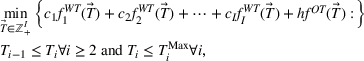

\begin{matrix} \min_{\vec{T} \in Z_{+}^{I}} \{c_{1} f_{1}^{WT} (\vec{T}) + c_{2} f_{2}^{WT} (\vec{T}) + \dots + c_{I} f_{I}^{WT} (\vec{T}) + h f^{OT} (\vec{T}) :\} \\ T_{i - 1} \leq T_{i} \forall i \geq 2 and T_{i} \leq T_{i}^{Max} \forall i, \end{matrix}

1where

c_{i}

is the unit daily (or weekly) wait time cost for priority class i patients, h is the overtime cost per patient, and I is the number of patient classes. The functions

f_{i}^{W T} (\vec{T})

and

f^{O T} (\vec{T})

represent the average wait time for priority class i patients and the average daily (or weekly) overtime utilization, respectively. The vector

\vec{T} = (T_{1}, T_{2}, …)

is a decision variable that represents the wait time targets and

{\vec{T}}^{Max} = (T_{1}^{Max}, T_{2}^{Max}, …)

is the vector of maximum clinically recommended wait times. We assume that lower values of i represent higher priority patients, and thus the targets should be nondecreasing in i.

An important caveat to note is that we are assuming that a clinic has already done its due diligence in ensuring sufficient (but not excess) available capacity in order to meet demand. If this first step is not done then the setting of targets is largely a pointless task as indeed is spending much time determining a good scheduling policy. In a setting with excess capacity, even a first‐come‐first‐served policy will likely be fine and achieving wait time targets will not be much of an issue. Conversely, in a setting where there is insufficient capacity, no scheduling policy will be capable of achieving any targets in the long run. A clinic that continually finds itself having to adjust its wait time targets is likely one that needs to go back and revisit the capacity decisions made earlier. Of course, it is in that narrow band where there is sufficient capacity but not excessive capacity that a clinic is functioning most efficiently. Thus, this paper focuses on a setting where capacity is about equal to average demand. The presence of overtime allows such a system to function well provided that the scheduling policy is a good one and the targets are well set.

The use of average as the metric related to wait times needs some justification as, quite frequently, health organizations prefer to focus on the 90th percentile. We focus on averages because we are attempting to balance the “cost” of waiting against the cost of overtime. Thus, we are interested in the wait time of the average patient rather than that of the extreme value represented by the 90th percentile. The challenge with using the 90th percentile is that it introduces intractable nonlinearity to the problem. Moreover, there are a number of reasons why we believe the analysis using averages is sufficient. First, we consider a scheduling policy that does not book patients late meaning that the wait time targets act like hard upper limits on the wait time of patients thus providing a bound on the 90th percentile (assuming that the capacity has been determined as mentioned earlier and that sufficient overtime is available). This follows from earlier research (Sauré et al., 2015) demonstrating that booking patients late rarely has any benefit because all it does is to push the problem downstream rather than addressing it. Second, we explicitly state that the final targets must be less than or equal to the clinically acceptable maximums thus ensuring that the wait time of the 90th percentile is within acceptable limits. It is certainly true that the cost of waiting is likely nonlinear past the clinical acceptable maximums as those targets are precisely the point at which, in the judgment of clinicians, the health of the patient begins to deteriorate rapidly. However, within those upper bounds it is reasonable to assume that the health of the patient does not deteriorate too quickly and thus the cost of waiting can reasonably be captured using the average. Third, our method proposes wait time targets where the implicit cost of waiting has been reduced to zero as the implication is that there is no further reduction in overtime possible by extending them further (given the available capacity, demand distribution and the scheduling policy implemented). It stands to reason that the point at which the implicit cost of waiting for the 90th percentile reaches zero would be as low or lower than that point determined by using the average leading to an even more aggressive reduction in the targets. The only alternative to our approach currently available to clinics is to maintain the targets at the clinically acceptable maximums that would clearly increase the 90th percentile wait times compared to our approach. All that notwithstanding, we acknowledge that the use of averages may be seen as a limitation of our approach.

There are several challenges that prevent us from directly solving (1). First, average wait times and overtime utilization depend on the demand, the system capacity and the scheduling policy employed. Second, even if the demand, system capacity and scheduling policy are known, there is no closed‐form expression for either the average wait times or the overtime function. Finally, even if there were functions that accurately captured the average wait times, there are no objective values for the unit wait time costs

c_{i}

in the objective function. We emphasize that what we are providing in this research is a methodology that determines wait time targets that are setting specific. In the following subsections, we therefore suggest the following approach to determine the best choice of wait time targets that addresses the challenges laid out above:

Determine the setting. This requires three tasks. (a)

Choose an intelligent scheduling policy. We briefly describe some advance patient scheduling policies available in the literature that have previously been shown to perform well. From these policies, we choose a single booking policy to use for the rest of the paper. The choice of this policy is justified below but the method itself could be utilized based on any other policy. An organization using a different scheduling policy would simply need to adjust the simulation component (step 3 below) of the methodology accordingly.

(b)

Ensure that sufficient capacity (both regular and overtime) is available to make the scheduling policy viable. For instance, the policy that we use in the rest of the paper books within the targets and uses overtime if no such capacity is available. Thus, the demand distribution imposes a capacity requirement. Previous research provides one means of determining the necessary capacity (Patrick et al., 2008).

(c)

Determine distribution of demand for each priority class.

Simulate the setting. Once the setting is known (step 1) simulate the chosen scheduling policy under the known capacity and demand for a wide set of potential wait time targets.

Approximate the average wait time and overtime functions. Based on the simulated data, approximate the average wait time for each priority class and the average overtime as a function of the choice of wait time targets using either multiple regression or neural networks.

Forward optimization problem. Formulate the forward optimization (FO) problem described in (1). As solving this problem relies on knowing subjective wait time costs, we move to step 5 as a means to implicitly determine these costs.

Inverse optimization problem. Use inverse optimization to determine the implicit wait time costs associated with the choice of a given set of targets (rather than imposing an arbitrary cost). In inverse optimization, the goal is usually to infer the parameters of the FO, intending to later solve that FO with the inferred parameters. Here, the end goal is rather to use inverse optimization as a middle step toward finding targets that are then used in conjunction with the scheduling policy. To that end, we demonstrate that, for each priority class, there comes a point where the implicit cost of waiting has been reduced to zero. This represents the target beyond which there is no managerial benefit (i.e., no reduction in overtime) achieved by extending the target further.

Set the targets. Recommend as the wait time target for each priority class the minimum of the clinically acceptable maximum and the point where the implicit cost of waiting has been reduced to zero.

These steps are outlined in the following sections using numerical examples throughout to illustrate.

Determine the setting

Choosing a scheduling policy

Advance patient scheduling plays a critical role in the optimal allocation of capacity among different types of incoming patients. There are several advance scheduling policies discussed in the literature. Using a first available slot policy (i.e., a myopic policy based on the immediate cost function), patients are booked as soon as possible in order of urgency. This policy fails to consider the impact of today's decisions on the future performance of the scheduling system. Patrick et al. (2008) derived a set of booking rules known as the PPQ (Patrick, Puterman, and Quayrenne) policy to efficiently book incoming patients into available appointment slots. According to this policy, the highest priority patients are booked as soon as possible within the wait time target and lower priority patients are booked on day 1, then on the last day within the target window and finally working backward to day 2. If there is insufficient capacity within the target window, overtime is used rather than booking late. More recently, Sauré et al. (2015) compared the performance of several advance scheduling policies including a novel SS policy (policy obtained through a simulation‐based approximate dynamic programming approach using an S‐shaped value function approximation), the PPQ policy, a Myopic policy, and a heuristic policy called “Day with the Minimum Number of Bookings” or DMB policy. The DMB policy books patients on day 1 and then on the day within the target window that contains the fewest bookings—starting with the highest priority class and working downward. If the capacity within the target window is insufficient, overtime is used. The Myopic policy performed very poorly compared to the others on most relevant metrics (such as total discounted cost, average wait times, average time to first available slot, percentage of late bookings and overtime utilization) while the performance of the DMB and the PPQ were reasonably similar with the notable exception that the DMB managed significantly lower average wait times for the lower priority classes. Although the SS policy outperformed both the PPQ and the DMB, the improvement was small. The significant downside of the SS policy is that it depends on an optimization model rather than a set of policy rules thus making it much more difficult to implement. Considering both performance and practicality, we chose to simulate the DMB policy to approximate the average wait times and overtime utilization as functions of the different wait time targets though again the approach can be used with any policy. To demonstrate the latter, we provide one example where the first available slot policy (with booking limits) is used instead.

Demand and capacity

We describe the proposed approach using several multi‐priority patient scheduling settings including three illustrative examples with two patient classes (base case and two variants) and a practical application with four patient classes. For the illustrative examples, we consider a small clinic with an average daily demand of 10 appointment requests per day, regular‐hour capacity of 10 appointment slots per day, and sufficiently high overtime capacity to serve all the demand not booked through regular‐hour capacity (four slots suffice). First, we assume that the clinic classifies incoming patients into two categories, priority 1 and 2, with maximum clinically recommended wait times of 7 and 14 days, respectively (i.e.,

{\vec{T}}^{M a x} = [7, 14]

). The daily demand of each type is assumed to follow a Poisson distribution with means of 7 and 3 requests per day, respectively. In addition, and for comparative purposes, we present the results from two variants of the two‐patient class setting. In the first variant, patients are scheduled using the first available slot policy rather than the DMB. In the second variant, the system is assumed to be under‐capacitated (imbalanced) with regular‐hour capacity for nine appointments per day but demand remaining at an average of 10 appointment requests per day. We intentionally chose decreasing demand rates for the illustrative examples as the demand rates increase for lower priority patients in the practical application we describe next. This enabled us to explore the impact of both increasing and decreasing demand patterns on the choice of wait time targets. The practical application is based on data from a rheumatology clinic at a large teaching hospital in Ontario, Canada. The clinic receives an average of 39 new‐consult requests per week from patients classified into five priority classes. The maximum clinically recommended wait times are 2, 9, 13, 26, and 52 weeks, respectively. To simplify the analysis of the simulation results, we combined the demand for consults coming from the last two classes and assumed a joint maximum clinically recommended wait time of 26 weeks (i.e.,

{\vec{T}}^{M a x} = [2, 9, 13, 26]

). Consequently, we consider weekly Poisson service requests with rates of 0.78, 7.41, 13.26, and 17.55 for patients of priority 1, 2, 3, and 4, respectively.

Simulate the setting

The simulation of the settings outlined in Subsection 3.1 involved a warm‐up period of

T_{0} = 250

days and a simulation length of

T = 1250

days. Results are averaged over

R = 30

replications. We tested the performance of the booking policy over all possible wait time target values lower than the corresponding maximum medically recommended wait times and computed the following output measures: average wait time (in days or weeks) per patient for each priority class and average volume of overtime bookings (per day or week) aggregated across all priority classes. The simulation model was implemented in Java and run on a MacBook Pro computer with a 2.4 GHz Intel Core i7 processor and 16 GB of RAM. A pseudo‐code of the simulation procedure for the two‐patient class example is provided in Algorithm 1.

ALGORITHM 1

Simulation procedure for the two‐patient class example

Require: $T_{1}^{Max} \geq 1$ and
$T_{2}^{Max} \geq 1$
, where
$T_{1}^{Max} \leq T_{2}^{Max}$

$T_{0} \leftarrow$
length of the warm‐up period

$T \leftarrow$
length of a simulation run for statistics collection

$R \leftarrow$
number of replications

$λ_{1}, λ_{2} \leftarrow$
demand rates

for
$i \leftarrow 1$
to
$T_{1}^{Max}$
do

for
$j \leftarrow i$
to
$T_{2}^{Max}$
do

$r \leftarrow 0$

repeat

for
$t \leftarrow 1$
to
$T_{0} + T$
do

Generate random Poisson demand with rates λ₁ and λ₂

Book appointments according to the chosen patient scheduling policy (e.g., DMB policy)

end for

return Average wait time and total overtime bookings over days
$[T_{0} + 1, T]$

$r \leftarrow r + 1$

until
$r = R$

end for

end for

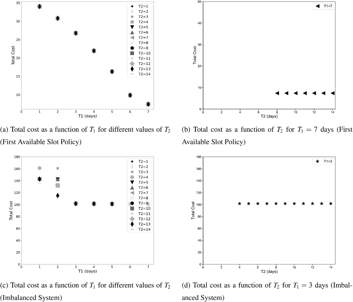
Figure 1 displays some of the results of the simulation for the base‐case example with two patient classes. In this setting, the mean wait times increase linearly with T ₁ and T ₂ as shown in Figure 1a,b. According to Figure 1b, the rate of increase of the mean wait for priority 2 patients increases as a function of T ₁ and achieves its lowest value when
$T_{1} = 1$
. This intuitively makes sense as a lower wait time target for priority 1 patients means that priority 1 patients are served more frequently through overtime leaving more available capacity for priority 2 patients. Figure 1c depicts the nonlinear relationship between the mean number of overtime bookings per day and the wait time target for the priority 2 class, for each value of T ₁. The graph shows a sharp drop in mean overtime utilization as the wait time targets are increased, particularly for the highest priority class, followed by an almost constant mean overtime level after the targets reach a certain point. This confirms the suspicion that there is a diminishing rate of return in terms of mean overtime reduction as the wait time targets are increased. Simulation results for the other settings are omitted because they provide similar conclusions.

FIGURE 1
Simulation results of the DMB policy for two patient classes.

Approximate the average wait time and overtime functions

Having created a data set through simulation, we use multiple regression and a neural network method called a feed‐forward multi‐layer perceptron (MLP) to obtain the functional representations
$f_{i}^{W T} (\vec{T})$
and
$f^{O T} (\vec{T})$
of the relationship between the wait time targets, denoted by
$\vec{T}$
, and the average wait times and the overtime utilization, respectively. It is important to note that there is a clear trade‐off between performance and interpretability with respect to model selection. On the one hand, multiple regression models are intuitive and can result in a good predictive performance. On the other hand, neural network approaches including feed‐forward MLP models are less intuitive and interpretable (i.e., typically a black box) but more capable of capturing the complex nonlinear relationship between input and output variables.

To obtain closed‐form functions to approximate the average wait times (in days or weeks) and the average number of overtime bookings (per day or week) as a function of the wait time targets, we proceed according to the following step‐wise procedure. In each case, we first fit a multiple linear regression model, and if the goodness‐of‐fit measure, the
$R_{adj}^{2}$
, is satisfactory, we stop. Otherwise, we expand the multiple linear regression model to include quadratic terms and thus incorporate nonlinearity into the modeling. Finally, we proceed to fit a feed‐forward MLP model if satisfactory predictive performance cannot be obtained with the linear and quadratic multiple regression models. By following this approach, we add an additional layer of complexity to the model until we get a reasonable approximation (e.g.,
$R_{adj}^{2} \geq 80 %$
). In addition to quadratic terms, we also considered two‐way interaction terms between the different wait time targets in a full second‐order multiple regression model. Although, some interaction terms were statistically significant at
$α = 0.05$
, the models did not show a meaningful increase in the
$R_{adj}^{2}$
. Further analysis showed that this mild interaction was only present for high values of the wait time target for the most urgent patient class. Because of the difficulties in drawing a meaningful interpretation for the corresponding coefficients, we omitted the two‐ and three‐way interaction terms in the final regression models. We use the R statistical software to conduct all the ordinary least‐squares multiple linear and quadratic regression analyses. The resulting model parameters and performance for the two‐ and four‐patient class settings are summarized in Table 2. For each setting, Table 2 provides either a multiple regression model or indicates an “MLP model”. The latter is done for settings where a neural network approach was required due to the poor fit obtained through multiple regression. Using multiple regression models, the
$R_{adj}^{2}$
values for the average wait time functions were over 90% for all cases except for the mean wait time for priority 1 patients in the four‐patient class setting. However, the
$R_{adj}^{2}$
values for the average overtime functions were typically lower. We therefore implemented neural network models to estimate average overtime as a function of the different wait time targets.

TABLE 2
Mean wait time and mean overtime function parameters.

Outcome Intercept $T_{1}$
$T_{2}$

$T_{3}$

$T_{4}$

$T_{1}^{2}$

$T_{2}^{2}$

$T_{3}^{2}$

$T_{4}^{2}$

$R_{adj}^{2}$

Two patient class (base case)

MWT, Pr. 1 0.436 0.474 −0.007 99.1%

MWT, Pr. 2 −0.982 0.512 0.630 93.8%

MOPD 1.100 −0.285 −0.066 0.028 0.003 83.0%

Two patient class (first available slot)

MWT, Pr. 1 1.378 0.542 99.9%

MWT, Pr. 2 1.970 0.539 99.9%

MOPD 0.235 −0.051 0.004 99.1%

Two patient class (imbalanced system)

MWT, Pr. 1 0.828 −0.014 98.7%

MWT, Pr. 2 −0.877 0.357 0.802 94.5%

MOPD Multi‐layer perceptron model—Two Layers with six neurons each 83.6%

Four patient class (rheumatology clinic)

MWT, Pr. 1 Multi‐layer perceptron model—Two layers with four neurons each 97.8%

MWT, Pr. 2 0.701 0.215 −0.003 −0.003 95.1%

MWT, Pr. 3 −0.524 0.058 0.215 0.497 −0.020 96.8%

MWT, Pr. 4 −2.230 0.092 0.117 0.212 0.848 99.3%

MOPW Multi‐layer perceptron model—Three layers with four neurons each 93.8%

Abbreviations: MOPD, mean overtime per day; MOPW, mean overtime per week; MWT, mean wait time; Pr, priority.

We used Python and the Keras/Tensorflow machine learning framework library to fit MLP models. The model building process involved a total of 280 observations for the two‐patient class imbalanced system and 3944 observations for the four‐patient class rheumatology clinic case. We used a 70%–15%–15% data set split for model training, validation and testing, respectively.

One of the key tasks when working with neural networks is hyper‐parameter tuning. There are several approaches to perform this task, including manual search, grid search, random search and Bayesian optimization methods. In our case, we observed the trained models to be robust to key hyper‐parameter changes on the validation data sets. Consequently, and given the scale and focus of the problem at hand, we deemed manual experimentation to be satisfactory for the purpose of our study. Through manual testing one can quickly test a choice of parameters and their score, train the model again, and check the difference in the score, without the use of automation in the selection of parameters as required in a grid or random search (Mudugandla, 2019). Using the manual tuning approach, we determined the minimal number of neurons, epochs, and layers, together with the batch size that provided reasonable model validation and prediction performance for each specific setting. We used rectified linear unit (ReLU) activation functions at each input and hidden layer and a linear activation function at the output layer. The latter was done to keep the model linearizable as linearity is crucial to accomplish the next step in our method that involves the formulation and solution of an inverse optimization model. The MLP model parameters for the two‐patient class and the four‐patient class settings are summarized in Tables 3, 4, and 5.

TABLE 3
Scaled MLP parameters for MOPD for the two‐patient class setting (imbalanced system).

Input layer Output layer

Weights Bias Weights Bias

−0.475 −0.557 0.172 0.961 0.029

−0.452 0.004 0.075 1.122

−0.466 −0.014 0.084 0.839

−0.024 −0.036 0.000 −0.526

−0.585 −0.036 0.134 0.945

0.131 −0.004 0.084 −0.162

TABLE 4
Scaled MLP parameters for MWT, Pr.1 for the four‐patient class setting.

Input layer Output layer

Weights Bias Weights Bias

0.098 0.193 1.398 2.158 0.094 0.097

−0.124 −1.095 0.115

−0.007 0.005

0.045 −0.032

TABLE 5
Scaled MLP parameters for MOPW for the four‐patient class setting.

Input layer Output layer

Weights Bias Weights Bias

0.004 −0.071 −0.004 0.001 −0.111 0.037

0.039 −0.316 −0.056 0.274 2.606

0.102 −1.302 −0.161 0.085 1.171

0.166 −3.566 −0.136

The forward optimization problem

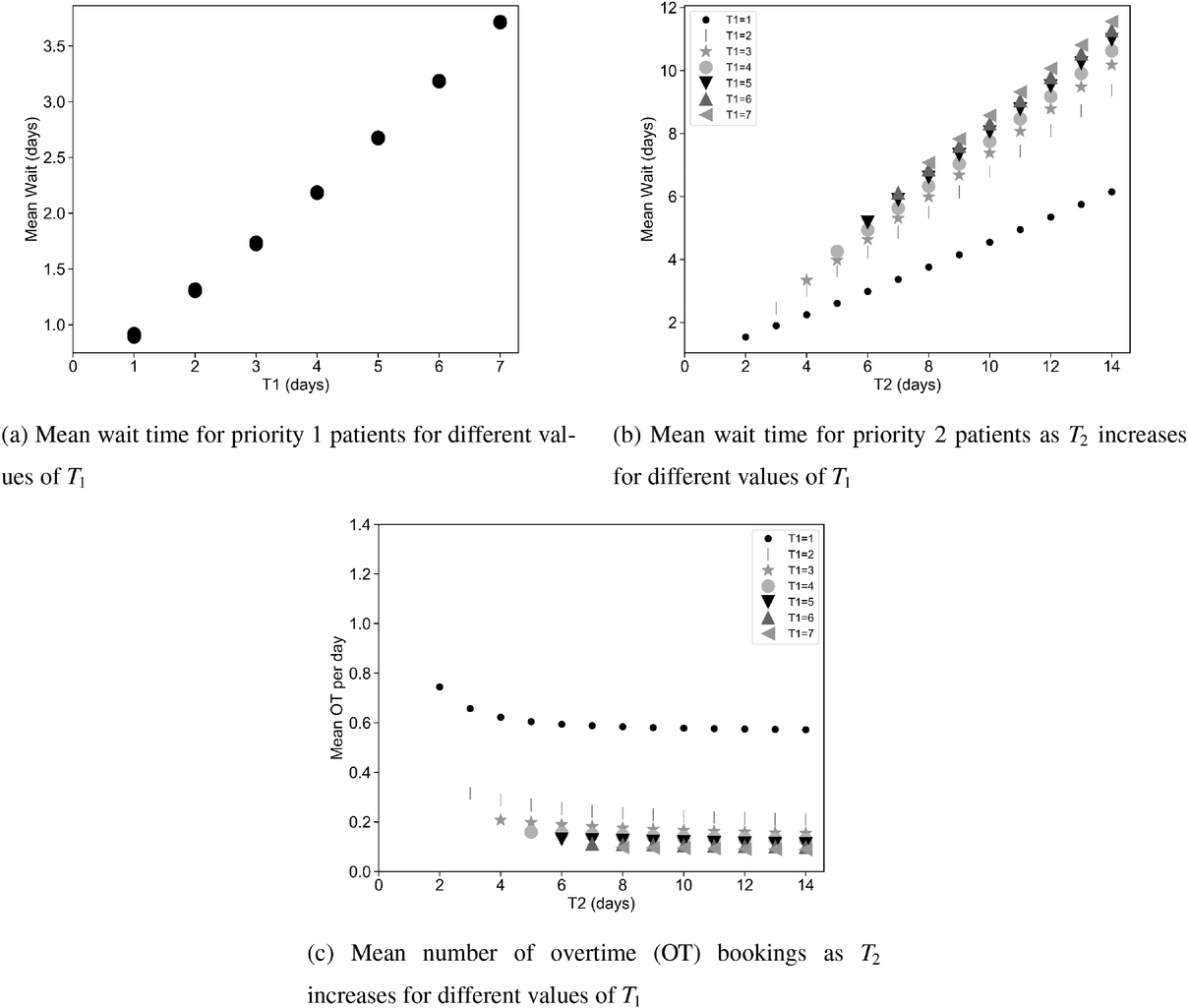
Using the parametric cost function in (1), we can now formulate a forward optimization problem in standard form denoted by “FO”. The corresponding model uses the parametric functions for the average wait times and the overtime bookings determined above. The constraints ensure that the wait time targets are nondecreasing with respect to priority class and that they respect the maximum clinically acceptable wait time for each patient group. The generic forward optimization model is given below.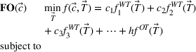
$\begin{matrix} FO (\vec{c}) & \min_{\vec{T}} f (\vec{c}, \vec{T}) = c_{1} f_{1}^{WT} (\vec{T}) + c_{2} f_{2}^{WT} (\vec{T}) \\ + c_{3} f_{3}^{WT} (\vec{T}) + \dots + h f^{OT} (\vec{T}) \\ subject to \end{matrix}$
2
$\begin{matrix} g_{m} (\vec{T}) \leq 0 m = 1, …, 3 I - 1, \end{matrix}$
3where, as mentioned earlier,
$c_{i}$
is the unit wait time cost for patient class i,
$f_{i}^{W T} (\vec{T})$
is the average wait time for patient class i,
$f^{O T} (\vec{T})$
is the average overtime utilization, and I is the number of patient classes. Additionally,
$g_{m} (\vec{T})$
is the mth constraint on the wait time targets. For example
$g_{i} = T_{i} - T_{i}^{Max}$
ensures that the maximum clinically recommended wait for priority class i is respected and
$g_{i} (\vec{T}) = T_{i - 1} - T_{i}$
ensures that the wait time target for priority class i is at least as large as the wait time target for priority class
$i - 1$
. Note that if a minimum difference between targets is desired then the above equation could simply be replaced by one that enforces the desired difference. Similarly, a maximum difference between targets could be enforced by adding an additional
$g_{i}$
function. Assuming a fixed unit cost of
$h = 100$
for each overtime booking, the explicit formulation for the two‐patient class setting is given in EC.1 in the Supporting Information.

To illustrate the approach when multiple regression does not provide a good approximation and a neural network formulation is required, we use the imbalanced variant of the two‐patient class setting. The ReLU activation function
$y = f (x) = \max (x, 0)$
used to derive the approximation functions in the MLP approach is continuous everywhere but not differentiable at
$x = 0$
, making the forward optimization model nonlinear and the direct application of the Karush–Kuhn–Tucker (KKT) conditions (required in the inverse optimization framework discussed later) impossible. Therefore, we first linearize the ReLU functions and transform the piece‐wise linear functions generated via the neural network approach into a set of equivalent linear constraints. The training performance of neural network models is superior when predictors and outcome variables are normalized. We used the min–max scaler function available in the sklearn library in Python to scale all the values between zero and one. Weight and bias parameters reported in Tables 3, 4, and 5 are obtained using scaled wait time target values, average wait times and average overtime utilizations. The values are transformed back before being inserted into (2).

In the imbalanced variant of the two patient class setting, the mean overtime per day (MOPD) is approximated using a feed‐forward MLP with six neurons in the input layer leading to six pairs of constraints in the linear program. Thus, the forward optimization problem for this setting can be formulated as shown in EC.5 in the Supporting Information. The forward optimization formulations for the other settings are derived in much the same manner.

Inverse optimization

The above sections provide an approach to determine reasonable parametric functions for the average wait time for patients of each priority class and for the average number of overtime bookings for a given demand, system capacity and scheduling policy. However, in order to determine the best choice of wait time targets using (1) one would also need to know the cost parameters associated with patient waiting,
$c_{1}, …, c_{I}$
. These remain difficult to quantify. Rather than attempting to quantify them, we use inverse optimization to determine the implicit cost of waiting imposed by a given choice of wait time targets. We then look to find the point where the implicit cost of waiting has been driven to zero. This represents the point at which any further increase in the target provides no managerial benefit. If this is less than the clinically acceptable maximum then it makes sense to reduce the target to this point rather than extending patient waiting unnecessarily. If this point is past the clinically acceptable maximum then this provides reason for the clinic to re‐consider the clinical maximum for this class and/or reduce the proportion of demand that class contains. If neither of those options is medically advisable, then the clinically maximum simply represents the best target.

Inverse optimization seeks to determine the cost parameters associated with the forward problem that render a given feasible solution optimal or approximately optimal. Inverse optimization has a wide range of applications including but not limited to finance (Bertsimas et al., 2012), health care decision‐making (Erkin et al., 2010), cancer treatment planning (Chan et al., 2014), and energy markets (Birge et al., 2017). Ahuja and Orlin (2001) discuss the general methodological framework for inverse problems under the L ₁ and
$L_{\infty}$
norms. Iyengar and Kang (2005); Zhang and Xu (2010) and, more recently, Keshavarz et al. (2011) provide an inverse optimization framework for convex programs. Their approaches are based on satisfying (approximately) the KKT necessary and sufficient optimality conditions with some residuals denoted by epsilon (ε). The ε approach determines the cost parameter values that make an observed solution approximately satisfy the KKT optimality conditions (Bertsimas et al., 2012; Chan et al., 2014; Keshavarz et al., 2011). Using this framework, the generic inverse optimization model, denoted by “IO,” takes the following form:
$\begin{matrix} IO (\vec{T}) \min_{\vec{ε}} ∥ \vec{ε} ∥_{1} = \sum_{i = 1}^{I} | ε_{i}^{1} | + \sum_{m = 1}^{3 I - 1} | ε_{m}^{2} | \end{matrix}$
4subject to
$\begin{matrix} \nabla f (\vec{c}, \vec{T}) + \sum_{m} λ_{m} \nabla g_{m} (\vec{T}) + ε_{i}^{1} & = 0 & i = 1, …, I, \end{matrix}$
5
$\begin{matrix} λ_{m} g_{m} (\vec{T}) + ε_{m}^{2} & = 0 & m = 1, …, 3 I - 1, \end{matrix}$
6
$\begin{matrix} g_{m} (\vec{T}) & \leq 0 & m = 1, …, 3 I - 1, \end{matrix}$
7
$\begin{matrix} λ_{m} & \geq 0 & m = 1, …, 3 I - 1, \end{matrix}$
8
$\begin{matrix} c_{i} & \geq c_{i + 1} & i = 1, …, I - 1, \end{matrix}$
9
$\begin{matrix} c_{i} & \geq 0 & i = 1, …, I . \end{matrix}$
10

In the inverse optimization model IO
$(\vec{T})$
, the elements of the vector
$\vec{T}$
, denoted by
$T_{i}$
, represent observed candidate solutions. Constraint (5) corresponds to the KKT stationarity conditions obtained by making the gradient of the Lagrangian with respect to each element of vector
$\vec{T}$
equal to zero, where
$λ_{m}$
is the Lagrangian dual variable (or multiplier) associated with the mth constraint in the primal (i.e., forward) problem. Constraint (6) corresponds to the complementary slackness conditions. To ensure dual feasibility of the inverse model, we include residual terms in the stationarity and complementary slackness conditions. These terms, unrestricted in sign, are minimized in the objective function. Constraints (7) and (8) correspond to the primal and dual feasibility conditions, respectively. In addition, in constraints (9) and (10), we assume that the elements of a feasible unit wait time cost vector
$\vec{c}$
are nonnegative and monotonic in relation to one another. It is important to note that although we impute the objective function based on integer wait time target values, we do not constrain the decision variables in the above forward and inverse optimization models to be integer because noninteger (i.e., continuous) wait time target values have practical interpretation too.

In EC.2 in the Supporting Information, we provide the explicit formulation of the IO model for the case of two patient classes with average wait time and overtime utilization functions derived using multiple regression. The IO model for the case of two classes with an MLP‐derived FO objective function is given in EC.6 in the Supporting Information. As a total of six neurons were used in the input layer of the MLP, 12 additional constraints are required. The coefficients in the inverse optimization model constraints are obtained by applying the KKT conditions to the primal (i.e., forward) optimization problems in EC.1 and EC.5 in the Supporting Information. The inverse optimization models for the other cases are derived in much the same manner.

Convexity

The validity of the above approach depends on the convexity of the mathematical programs. In this section, we demonstrate that convexity. Proposition 1
Primal objective functions that are affine, quadratic or a combination of both are convex in the wait time targets.

Proof 1
The proof is trivial. Using the convexity properties of affine and quadratic functions with positive quadratic terms, one can show that the average wait time and overtime functions are convex in the wait time targets. In addition, a nonnegative weighted sum of convex functions
$(c_{i} \geq 0 \forall i)$
is also convex resulting in an overall convex cost function. Alternatively, using the second‐order necessary and sufficient conditions of convexity, one can easily show that primal objective functions are convex. In other words, the Hessian matrix is positive semi‐definite.
$□$

Remark 1
Due to the convexity property of norms, the objective functions associated with the inverse optimization problems are also convex (Boyd et al., 2004).

Remark 2
Both primal and dual problems satisfy Slater's constraint qualifications. Under Slater's rule, the KKT conditions are both necessary and sufficient for optimality (Boyd et al., 2004).

Corollary 1
It is important to note that Proposition 1 and remarks 1 and 2 ensure that a local optimal solution to the nonlinear forward and inverse optimization models will also be a global optimal solution (Boyd et al., 2004).

The IO models seek to minimize
$∥ \vec{ε} ∥_{1}$
, the L ₁‐norm of vector ε (also known as the Manhattan norm). As the absolute value function is a convex nonlinear function, we replaced
$ε_{i}$
by
$ε_{i}^{+} - ε_{i}^{-}$
, where
$ε_{i}^{+} \geq 0$
and
$ε_{i}^{-} \geq 0$
, in all mathematical programs.

All the inverse optimization models in the paper were coded in Python and solved using Gurobi API on a MacBook Pro computer with a 2.4 GHz Intel Core i7 processor and 16 GB RAM. For practical reasons, we considered all integer feasible solutions for wait time targets. The models with two patient classes typically solved in under 15 s while the models with four patient classes solved within a minute.

Choose the wait time targets

We numerically solve the IO problem as described in Equations (4)–(10) for each setting and, based on the outcome, recommend wait time targets.

Two priority class setting with its two variants

For the base case of the two patient class setting (models in EC.1 and EC.2 in the Supporting Information), Figure 2a demonstrates that c ₁, the unit wait time cost for priority 1 patients, decreases monotonically as the value of T ₁ increases and that it quickly drops to zero past
$T_{1} = 5$
across different values of T ₂. For a fixed value of T ₂, the cost coefficient c ₁ attains its lowest value when
$T_{1} \geq 6$
and its highest when
$T_{1} = 1$
. At its peak, the cost of an additional day of wait for priority 1 patients is almost half the cost of an overtime slot while the cost of waiting for priority 2 patients is zero.

FIGURE 2
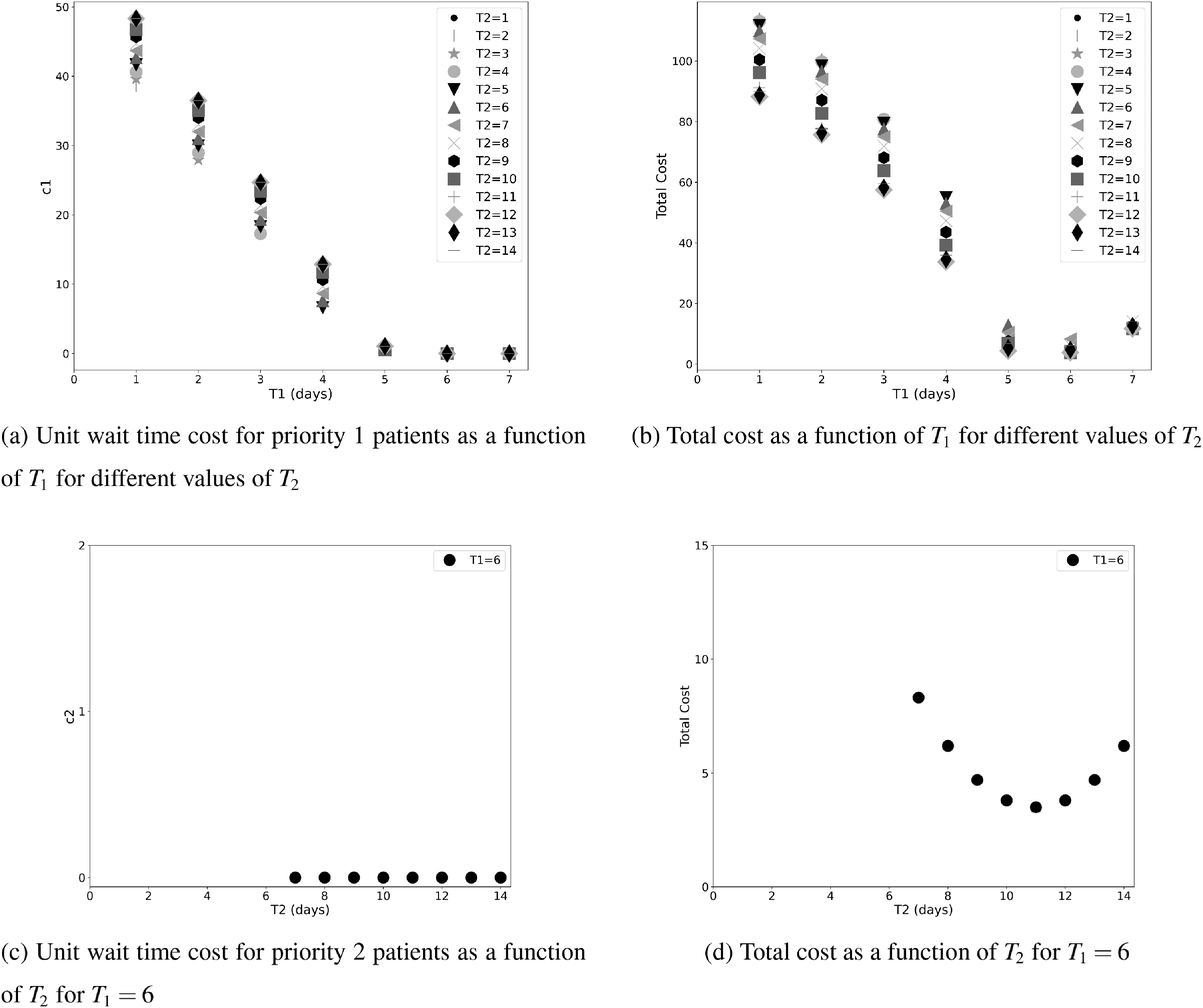
Unit wait time cost values (c ₁ and c ₂) and total cost for the clinical setting with two patient classes (base case).

The highest possible value for the cost of waiting for the second priority class is one tenth of the cost of an overtime slot and occurs when
$T_{1} = 1$
and
$T_{2} = 2$
(not shown). As the wait time target T ₂ increases, c ₂ decreases monotonically hitting the cost of zero at
$T_{2} = 11$
for T ₁ values ranging from 1 to 6 days. Figure 2b,d depicts the FO objective function values for different values of T ₁ and T ₂, respectively. The total system cost is minimized when
$T_{1} = 6$
(Figure 2b) and
$T_{2} = 11$
days (Figure 2d). Thus, for a clinic of this size, experiencing the given demand and utilizing the DMB policy, there is no positive choice of c ₁ and c ₂ that could justify increasing T ₁ and T ₂ beyond 6 and 11 days, respectively. Put in another way, one would have to place a positive value on patient waiting time in order to justify targets beyond 6 and 11 for this setting. Thus, in this case, the best choice of wait time targets are smaller than the clinical maximums of 7 and 14. It might seem counterintuitive to observe that the total cost goes up as the wait time targets increase because the unit wait time costs are zero for
$T_{1} \geq 6$
and
$T_{2} \geq 11$
. The explanation is simple and comes from the fact that the average overtime utilization is modeled as a quadratic function. Although it approximates the sharp decrease in the total cost values due to less overtime usage as the wait time targets increase, the function values go back up after hitting the global minimum, resulting in higher function approximation errors. Ideally, we would prefer an approximation function that captures the constant total cost past the minimum targets. That said, the point here is to show that the total cost does not improve beyond a certain threshold.

For the two patient class variant where patients are scheduled using the first available slot scheduling policy (models in EC.3 and EC.4 in the Supporting Information), we first need to determine the respective booking limits, which are defined as the number of days beyond the wait time targets when the cost of waiting becomes higher than that of overtime. This is typically done by dividing the unit overtime cost by the unit wait time cost associated with each priority class. In our case, however, the unit wait time costs are not known in advance. We chose 2 and 10 days (beyond the clinical maximums) as the booking limits for priority 1 and 2 patients, respectively. These values are based on the maximum costs of waiting determined through the use of the DMB policy for the two priority class setting (base case), which are approximately
$c_{1} = $ 50$
for priority 1 patients and
$c_{2} = $ 10$
for priority 2 patients when the overtime cost is $100. Then, the total cost attains its minimum value at
$T_{1} = 7$
days (Figure 3a), and it remains the same regardless of the value of T ₂ (Figure 3b). In other words, T ₂ does not help, statistically speaking, predict any of the terms in the objective function of the forward optimization problem (see Table 2). Thus, using a first available slot policy increases the wait time target of the highest priority class because it subsumes the priority 2 class into the first. This is intuitively reasonable as a first available slot policy essentially ignores the priority and thus needs a larger window to distribute patients. This demonstrates the impact of the size of a patient class as the larger the class the larger the window needed to maximally smooth out demand.

FIGURE 3
Total cost for the variants of the clinical setting with two patient classes (first available slot policy and imbalanced system).

In the imbalance case (models in EC.5 and EC.6 in the Supporting Information), the total cost is minimized when the value of T ₁ is 3 days and remains steady thereafter (Figure 3c). For the second class, any value of
$T_{2} \geq T_{1} = 3$
provides the same cost (Figure 3d). Thus, in a system with insufficient capacity, targets are actually shortened as overtime is inevitable. Idle time is unlikely leading to less benefit in pre‐filling the schedule and thus allowing the clinic to function with shorter wait time targets without increasing overtime costs (compared to a similarly imbalanced system with higher wait time targets) but, obviously, at a higher overtime cost than one sees in the (balanced) base‐case scenario. In an even more imbalanced system, targets would eventually become equal to one leading to an “open access” policy that serves all demand the day it arrives but with likely unacceptable levels of overtime.

Table 6 summarizes the simulation results obtained for each of the two priority class settings discussed above using both the clinical maximums and the targets recommended through our approach. Each set of wait times targets was simulated for 1250 days using common patient arrivals with statistics collected for each of 30 simulation runs after a warm‐up period of 250 days. Results confirm that the shorter targets determined through our approach provide lower wait times without increasing overtime.

TABLE 6
Simulation results for the two priority class settings.

Maximum recommended Proposed

Setting Patient priority Target MWT MOPD Target MWT MOPD

Base case 1 7 3.72 ± 0.24 0.09 ± 0.02 6 3.18 ± 0.18 0.10 ± 0.02

2 14 11.56 ± 0.27 11 9.05 ± 0.20

First available slot 1 7 5.26 ± 0.42 0.07 ± 0.02 7 5.26 ± 0.42 0.07 ± 0.02

policy 2 14 5.84 ± 0.45 7 5.84 ± 0.45

Imbalance system 1 7 5.64 ± 0.02 1.01 ± 0.04 3 2.58 ± 0.01 1.02 ± 0.04

2 14 12.80 ± 0.01 3 1.99 ± 0.02

Note: The resulting 95% confidence interval is provided for each statistic.

Abbreviations: MOPD, mean overtime per day; MWT, mean wait time.

Four priority classes: The rheumatology clinic

For the rheumatology clinic (models in EC.9 and EC.10 in the Supporting Information), the situation is a bit different. In this case, the proportion of demand is increasing as the priority decreases so that the lowest priority class has the highest demand. The highest priority class is actually quite small leading to a smaller target presenting less of a challenge. The size of the lower priority classes results in the cost of waiting determined by the IO problem approaching zero but never quite reaching it all the way up to the clinical maximums (Figure 4). One might therefore think that either the maximums are fine or else there is an argument for extending them even further. However, when one examines the value of the imputed wait time costs or similarly the reduction in overtime achieved by extending the targets, the benefit appears to be minimal. 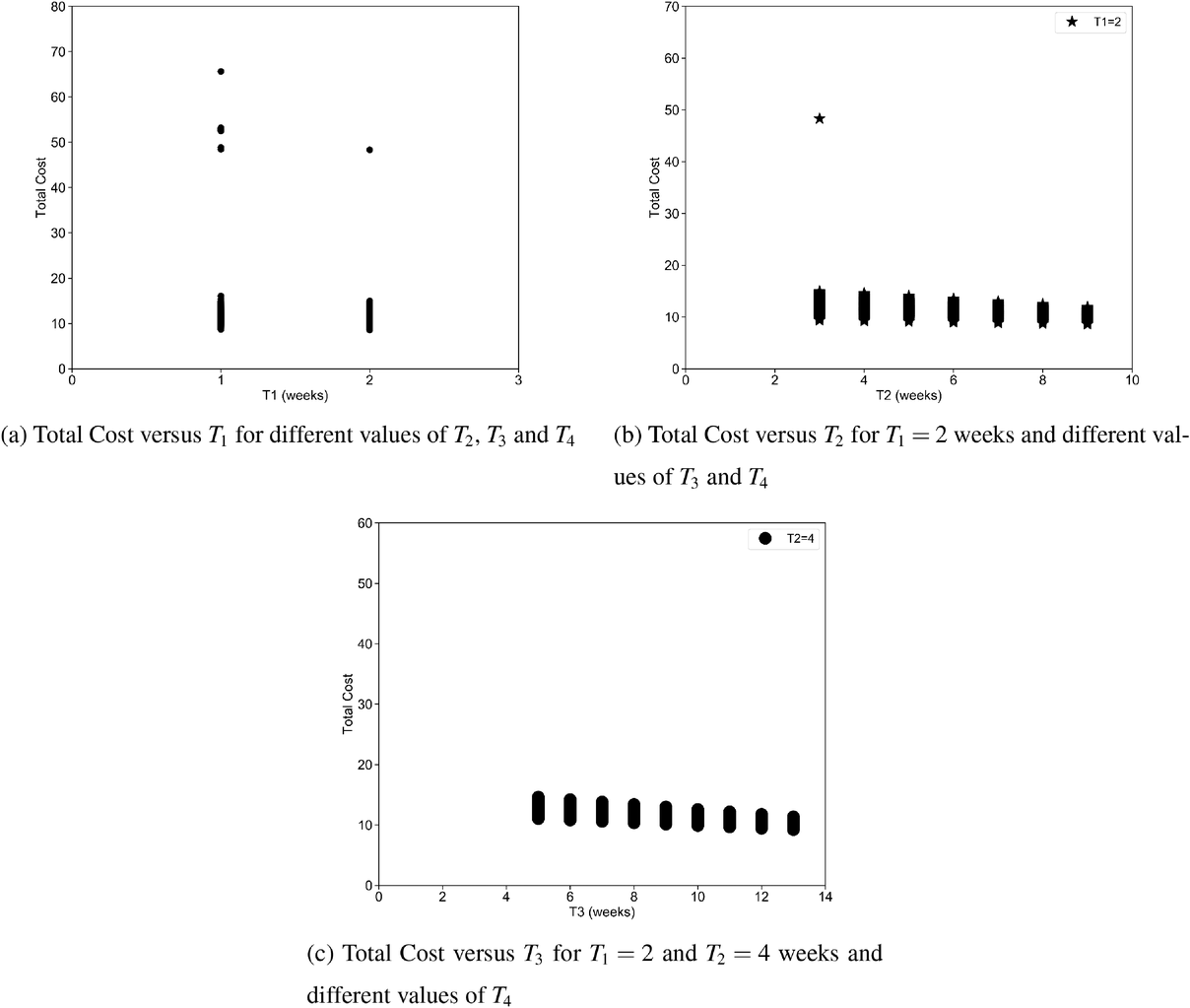For instance, if a clinic was to set the targets such that the chosen targets result in less than one additional overtime slot per year (assuming a 50 week year) when compared against the clinical maximums then any of the combinations provided in Table 7 are a possibility. These are deliberately chosen where each one demonstrates the smallest possible target value achievable for one of the priority classes that still increases OT by no more than one slot per year. This further demonstrates how aggressive targets for one class must be offset by less aggressive targets for another in order to ensure that sufficient flexibility in scheduling remains.

FIGURE 4
Total cost versus different wait time targets for a case study consisting of four priority classes.

TABLE 7
Simulation results for the rheumatology clinic.

Priority Target MWT MOPW MOPY increase

1 2 0.96 ± 0.02 0.0892 ± 0.0402 –

2 9 2.55 ± 0.51

3 13 7.95 ± 1.12

4 26 24.26 ± 0.51

1 1 1.00 ± 0.00 0.1079 ± 0.0403 0.935 ± 0.459

2 1 0.99 ± 0.01

3 13 4.92 ± 0.76

4 25 22.12 ± 0.78

1 2 0.96 ± 0.02 0.1063 ± 0.0400 0.857 ± 0.493

2 7 2.35 ± 0.38

3 7 3.89 ± 0.51

4 26 23.06 ± 0.82

1 2 0.95 ± 0.02 0.1067 ± 0.0406 0.876 ± 0.489

2 9 2.83 ± 0.48

3 13 8.59 ± 1.05

4 21 19.69 ± 0.48

Note: The resulting 95% confidence interval is provided for each statistic.

Abbreviations: MOPW/Y, mean overtime per week/year; MWT, mean wait time.

Thus if we are to stick to the approach outlined in this paper then the clinical maximums would remain the most appropriate targets. However clinics not concerned by a slight increase in overtime might consider more aggressive targets; representing a willingness to pay at least something (in increased OT) in order to reduce wait times to some degree.

A note on implementation

As mentioned earlier, implementation of our methodology requires that a clinic first do a proper demand analysis to ensure that they are not functioning with insufficient capacity. This is typically not a difficult task as it involves ensuring that the average demand of the clinic is equal to the available capacity. A more involved analysis using queuing theory to account for variability in demand is likely unnecessary provided the clinic has chosen an intelligent scheduling policy—such as the DMB utilized in this paper. Failure to do the required demand analysis and capacity planning will likely result in unacceptable levels of overtime. Furthermore, a clinic that has been using longer wait time targets than recommended by our method will undoubtedly need to go through a transition phase in order to bring the backlog of scheduled patients down to a point where the new targets can be maintained. For instance, a clinic moving from a target of 30 days to a target of 20 will have patients booked on days 21 to 30 who will need to be served through an additional outlay of resources (probably in the form of overtime). However, once this transition phase is completed, it is our contention that the cost of maintaining the more ambitious targets will be no more than what the clinic experienced prior to the transition.

DISCUSSION AND CONCLUSION

The goal of health care institutions is to provide the right care to patients in as timely a fashion as possible. In an effort to better define “timely”, governments have used expert opinion to determine priority‐specific, clinically acceptable wait time targets. However, rarely have governments or clinics done the necessary analysis to determine if those targets are manageable. What targets are manageable depends very much on the capacity available to an organization, the distribution of its demand (particularly the size of its highest priority class) and the scheduling policy employed. Thus, any attempt to determine appropriate priority‐specific targets need to be context specific and respect the upper bounds imposed by the clinical maximums.

In this paper we have provided just such a context‐specific approach to target setting. It is common for organizations struggling to meet their targets to seek relief by extending the target of the lowest priority class—a target that is often already quite long. What this research provides is a threshold on the target for each priority class beyond which there is no managerial benefit. If that threshold is lower than the clinical maximum then continuing to use the clinical maximum as the target simply imposes additional wait on the patient without justification. If, on the other hand, the threshold is higher than the clinical maximum then the clinic is in a situation where additional overtime is required as a result of the imposition of this clinical maximum. Such a clinic ought to explore whether that maximum is indeed appropriately set and further ensure that patients assigned to that priority class truly belong there. Extending the clinical maximum or limiting the size of this priority class can help reduce the amount of overtime required. Typically, it is higher priority classes with their shorter clinical maximums that cause this issue (unless the highest priority classes are very small such as in the rheumatology clinic example). Thus, contrary to popular practice, clinics ought to be focusing on the targets of the highest priority class rather than extending the target of the lowest class as it is the target of the highest priority class that drives the need for overtime.

Also contrary to popular thinking, our analysis demonstrates that an imbalanced system where average demand exceeds capacity actually has lower recommended targets than the balanced system. Although this can seem counterintuitive at first, there is a reasonable explanation. A system with more demand than capacity will run into the need for overtime much more quickly and experience idle time much less frequently. A shorter time window is sufficient to allow such a clinic to fill all regular hour capacity almost all the time. Targets can therefore be shorter without increasing overtime utilization. Again, we emphasize the importance a clinic should place on ensuring that capacity is at least equal to average demand prior to attempting to impose targets. Where capacity is insufficient, unacceptably high levels of overtime will be inevitable in order to meet any targets. If sufficient overtime is also not available, wait times will simply continue to increase and the targets become meaningless.

It is worth noting that our methodology to determine the optimal targets is general but the results presented in this paper are necessarily case specific as it is a distinct advantage of our approach that it takes into account the capacity, demand and scheduling policy employed. Generalizable results would defeat the purpose of providing targets that are achievable within a given setting. For example, it is insightful to note that classical regression models performed poorly for the rheumatology case study—most likely due to the fact that the lower priority classes constitute a high proportion of the total demand, whereas in the illustrative examples it was the highest priority class that accounted for most of the appointment requests. In addition, it is also important to note that having the first priority class accounting for the highest proportion of the total demand for service results in longer optimal wait time targets. This highlights the fact that the setting of targets needs to be case specific as what is reasonably achievable will depend on the capacity, the demand stream and the scheduling policy employed. Rather than replacing the consensus‐based approach, our approach provides a means to determine if the medically acceptable targets determined through the consensus approach are in fact necessary to achieve maximum managerial benefit. Thus, we ensure that patients do not wait longer than necessary to receive treatment.

As a future extension of this work, it would be worthwhile to evaluate the robustness of the results by considering different clinic sizes. In addition, one could argue that the demand for service depends on the wait time targets. For example, it would be reasonable to expect an increase in demand if a wait time target is set at 5 weeks instead of 26 weeks. If an improvement in wait times led to an increase in the number of appointment requests, it would be necessary to rerun the method with new operational parameters, which would likely result in slightly extended targets.

Table 1 demonstrates several examples of services with long clinical wait time targets for lower priority patients set through the consensus approach. As demonstrated using illustrative examples and a practical application, by utilizing the modeling approach in this paper we contend that many of the current wait time targets could be reduced significantly without requiring additional resources. Of course, it is certainly true that an initial outlay of resources would be required to reduce the wait lists to the point where the new targets can be maintained. Finally, our work highlights the important role that the scheduling policy and other operational factors such as demand and capacity play in determining what wait time targets are readily achievable.

The most notable benefit that can be obtained from the implementation of the proposed approach in clinical practice is the reduction of wait times in a systematic way ensuring timely patient access to care. As emphasized in the paper, this can be achieved through the use of good scheduling policies and accounting for specific demand and capacity values. To this end, the DMB policy is an easy to implement scheduling heuristic with provably better system and service level performance than other known policies in the literature. An appointment scheduling tool integrated to a patient information system could be used to implement the DMB policy and ensure efficient scheduling operations. To further automate the process, an integrated decision‐support tool with an optimization engine could be developed to assist with the determination of wait time targets based on the number of priority classes and the associated maximum recommended wait, demand rates and capacity parameters for a particular clinic.

Footnotes
ACKNOWLEDGMENTS
This work was partially supported by the Natural Sciences and Engineering Research Council of Canada (NSERC; Grants RGPIN‐2018‐05225 and RGPIN‐2020‐04301).
References
1.
Ahn H. Kreder H. Mahomed N. Beaton D. Wright J. G. (2011). Empirically derived maximal acceptable wait time for surgery to treat adolescent idiopathic scoliosis. CMAJ, 183(9), E565–E570.
2.
Ahuja R. K. Orlin J. B. (2001). Inverse optimization. Operations Research, 49(5), 771–783.
3.
Ansell D. Crispo J. A. Simard B. Bjerre L. M. (2017). Interventions to reduce wait times for primary care appointments: A systematic review. BMC Health Services Research, 17(1), 295.
4.
Astaraky D. Patrick J. (2015). A simulation based approximate dynamic programming approach to multi‐class, multi‐resource surgical scheduling. European Journal of Operational Research, 245(1), 309–319.
5.
Ballini L. Negro A. Maltoni S. Vignatelli L. Flodgren G. Simera I. Holmes J. Grilli R. (2015). Interventions to reduce waiting times for elective procedures. Cochrane Database of Systematic Reviews 2015, Issue 2 .
6.
Barua B. (2017). Waiting your turn: Wait time for health care in Canada, 2017 report, Fraser Institute.
7.
Barua B. Jacques D. (2019). The private cost of public queues for medically necessary care, 2019. Fraser Research Bulletin. Fraser Institute.
8.
Bertsimas D. Gupta V. Paschalidis I. C. (2012). Inverse optimization: A new perspective on the Black–Litterman model. Operations Research, 60(6), 1389–1403.
9.
Birge J. R. Hortaçsu A. Pavlin J. M. (2017). Inverse optimization for the recovery of market structure from market outcomes: An application to the MISO electricity market. Operations Research, 65(4), 837–855.
10.
Boyd S. Boyd S. P. Vandenberghe L. (2004). Convex optimization. Cambridge University Press.
11.
Cancer Care Ontario . (2019). Wait time targets. http://ocp.cancercare.on.ca/cms/One.aspx?portalId=327895&pageId=8870
12.
Chan T. C. Craig T. Lee T. Sharpe M. B. (2014). Generalized inverse multiobjective optimization with application to cancer therapy. Operations Research, 62(3), 680–695.
13.
Davis K. Stremikis K. Squires D. Schoen C. (2014). Mirror, mirror on the wall. How the performance of the US health care system compares internationally. New York: CommonWealth Fund.
14.
Derrett S. Paul C. Morris J. M. (1999). Waiting for elective surgery: effects on health‐related quality of life. International Journal for Quality in Health Care, 11(1), 47–57.
15.
Ding Y. Park E. Nagarajan M. Grafstein E. (2019). Patient prioritization in emergency department triage systems: An empirical study of the Canadian triage and acuity scale (CTAS). Manufacturing & Service Operations Management, 21(4), 723–741.
16.
Erkin Z. Bailey M. D. Maillart L. M. Schaefer A. J. Roberts M. S. (2010). Eliciting patients' revealed preferences: An inverse Markov decision process approach. Decision Analysis, 7(4), 358–365.
17.
Geng N. Xie X. (2016). Optimal dynamic outpatient scheduling for a diagnostic facility with two waiting time targets. IEEE Transactions on Automatic Control, 61(12), 3725–3739.
18.
Harrison A. J. Appleby J. (2009). English NHS waiting times: What next? Journal of the Royal Society of Medicine, 102(7), 260–264.
19.
Harrison A. J. Appleby J. (2010). Optimising waiting: A view from the English National Health Service. Health Economics, Policy and Law, 5(4), 397–409.
20.
Huang J. Carmeli B. Mandelbaum A. (2015). Control of patient flow in emergency departments, or multiclass queues with deadlines and feedback. Operations Research, 63(4), 892–908.
21.
Iyengar G. Kang W. (2005). Inverse conic programming with applications. Operations Research Letters, 33(3), 319–330.
22.
Kazemian P. Sir M. Y. Van Oyen M. P. Lovely J. K. Larson D. W. Pasupathy K. S. (2017). Coordinating clinic and surgery appointments to meet access service levels for elective surgery. Journal of Biomedical Informatics, 66, 105–115.
23.
Keshavarz A. Wang Y. Boyd S. (2011). Imputing a convex objective function. 2011 IEEE International Symposium on Intelligent Control (pp. 613–619), IEEE, Piscataway, NJ.
24.
Li S. Geng N. Xie X. (2015). Radiation queue: Meeting patient waiting time targets. IEEE Robotics & Automation Magazine, 22(2), 51–63.
25.
Liu N. (2016). Optimal choice for appointment scheduling window under patient no‐show behavior. Production and Operations Management, 25(1), 128–142.
26.
Luigi S. Michael B. Valerie M. (2013). OECD health policy studies. Waiting time policies in the health sector: What works? OECD Publishing.
27.
Ma X. Sauré A. Puterman M. L. Taylor M. Tyldesley S. (2016). Capacity planning and appointment scheduling for new patient oncology consults. Health Care Management Science, 19(4), 347–361.
28.
Mahon J. L. Bourne R. B. Rorabeck C. H. Feeny D. H. Stitt L. Webster‐Bogaert S. (2002). Health‐related quality of life and mobility of patients awaiting elective total hip arthroplasty: A prospective study. Canadian Medical Association Journal, 167(10), 1115–1121.
29.
Naiker U. FitzGerald G. Dulhunty J. M. Rosemann M. (2018). Time to wait: A systematic review of strategies that affect out‐patient waiting times. Australian Health Review, 42(3), 286–293.
30.
Olivares M. Terwiesch C. Cassorla L. (2008). Structural estimation of the newsvendor model: An application to reserving operating room time. Management Science, 54(1), 41–55.
31.
Paterson W. G. Depew W. T. Paré P. Petrunia D. Switzer C. vanZanten S. J. V. Daniels S. Canadian Association of Gastroenterology Wait Time Consensus Group . (2006). Canadian consensus on medically acceptable wait times for digestive health care. Canadian Journal of Gastroenterology and Hepatology, 20(6), 411–423.
32.
Patrick J. Puterman M. L. Queyranne M. (2008). Dynamic multipriority patient scheduling for a diagnostic resource. Operations Research, 56(6), 1507–1525.
33.
Robinson L. W. Chen R. R. (2011). Estimating the implied value of the customer's waiting time. Manufacturing & Service Operations Management, 13(1), 53–57.
34.
Sanmartin C. Gendron F. Berthelot J. M. Murphy K. (2004). Access to health care services in Canada, 2003. Statistics Canada.
35.
Sauré A. Patrick J. Puterman M. L. (2015). Simulation‐based approximate policy iteration with generalized logistic functions. INFORMS Journal on Computing, 27(3), 579–595.
36.
Sauré A. Patrick J. Tyldesley S. Puterman M. L. (2012). Dynamic multi‐appointment patient scheduling for radiation therapy. European Journal of Operational Research, 223(2), 573–584.
37.
Schaafsma J. (2006). Are there better ways to determine wait times? CMAJ, 174(11), 1551–1552.
38.
Mudugandla S. Y. (2019). 4 Hyper‐parameter tuning techniques and limitations. https://medium.com/swlh/4‐hyper‐parameter‐tuning‐techniques‐924cb188d199
39.
Zhang J. Xu C. (2010). Inverse optimization for linearly constrained convex separable programming problems. European Journal of Operational Research, 200(3), 671–679.
40.
Zhou L. Geng N. Jiang Z. Wang X. (2018). Multi‐objective capacity allocation of hospital wards combining revenue and equity. Omega, 81, 220–233.

Outcome	Intercept	$T_{1}$	$T_{2}$	$T_{3}$	$T_{4}$	$T_{1}^{2}$	$T_{2}^{2}$	$R_{adj}^{2}$
Two patient class (base case)
MWT, Pr. 1	0.436	0.474	−0.007					99.1%
MWT, Pr. 2	−0.982	0.512	0.630					93.8%
MOPD	1.100	−0.285	−0.066			0.028	0.003	83.0%
Two patient class (first available slot)
MWT, Pr. 1	1.378	0.542						99.9%
MWT, Pr. 2	1.970	0.539						99.9%
MOPD	0.235	−0.051				0.004		99.1%
Two patient class (imbalanced system)
MWT, Pr. 1		0.828	−0.014					98.7%
MWT, Pr. 2	−0.877	0.357	0.802					94.5%
MOPD	Multi‐layer perceptron model—Two Layers with six neurons each							83.6%
Four patient class (rheumatology clinic)
MWT, Pr. 1	Multi‐layer perceptron model—Two layers with four neurons each							97.8%
MWT, Pr. 2	0.701		0.215	−0.003	−0.003			95.1%
MWT, Pr. 3	−0.524	0.058	0.215	0.497	−0.020			96.8%
MWT, Pr. 4	−2.230	0.092	0.117	0.212	0.848			99.3%
MOPW	Multi‐layer perceptron model—Three layers with four neurons each							93.8%

Input layer			Output layer
Weights		Bias	Weights	Bias
−0.475	−0.557	0.172	0.961	0.029
−0.452	0.004	0.075	1.122
−0.466	−0.014	0.084	0.839
−0.024	−0.036	0.000	−0.526
−0.585	−0.036	0.134	0.945
0.131	−0.004	0.084	−0.162

		Maximum recommended			Proposed
Setting	Patient priority	Target	MWT	MOPD	Target	MWT	MOPD
Base case	1	7	3.72 ± 0.24	0.09 ± 0.02	6	3.18 ± 0.18	0.10 ± 0.02
	2	14	11.56 ± 0.27		11	9.05 ± 0.20
First available slot	1	7	5.26 ± 0.42	0.07 ± 0.02	7	5.26 ± 0.42	0.07 ± 0.02
policy	2	14	5.84 ± 0.45		7	5.84 ± 0.45
Imbalance system	1	7	5.64 ± 0.02	1.01 ± 0.04	3	2.58 ± 0.01	1.02 ± 0.04
	2	14	12.80 ± 0.01		3	1.99 ± 0.02

Priority	Target	MWT	MOPW	MOPY increase
1	2	0.96 ± 0.02	0.0892 ± 0.0402	–
2	9	2.55 ± 0.51
3	13	7.95 ± 1.12
4	26	24.26 ± 0.51
1	1	1.00 ± 0.00	0.1079 ± 0.0403	0.935 ± 0.459
2	1	0.99 ± 0.01
3	13	4.92 ± 0.76
4	25	22.12 ± 0.78
1	2	0.96 ± 0.02	0.1063 ± 0.0400	0.857 ± 0.493
2	7	2.35 ± 0.38
3	7	3.89 ± 0.51
4	26	23.06 ± 0.82
1	2	0.95 ± 0.02	0.1067 ± 0.0406	0.876 ± 0.489
2	9	2.83 ± 0.48
3	13	8.59 ± 1.05
4	21	19.69 ± 0.48

Setting wait time targets in a multi‐priority patient setting

Abstract

Keywords

INTRODUCTION

RELATED LITERATURE

A METHODOLOGY TO DETERMINE WAIT TIME TARGETS

Determine the setting

Choosing a scheduling policy

Demand and capacity

Simulate the setting

Approximate the average wait time and overtime functions

The forward optimization problem

Inverse optimization

Convexity

Choose the wait time targets

Two priority class setting with its two variants

Four priority classes: The rheumatology clinic

A note on implementation

DISCUSSION AND CONCLUSION

Footnotes

ACKNOWLEDGMENTS

References