
Abstract
How do firms respond after being exposed to a low‐probability, high‐consequence (lp‐hc) disruption event? This study examines inventory and flexibility patterns in manufacturing firms in the years following an lp‐hc event, the Great East Japan Earthquake of 2011. We find patterns suggesting that most firms exposed to the event began to increase their raw material inventories (RAW) over the longer term and increased their volume flexibility for a shorter period. Furthermore, we found that firms increased their RAW mainly when inventories were already at high levels, while the opposite is true for volume flexibility. Firms that were classified as risk‐averse before the event show stronger swings after the event. Preliminary explorations suggest that the performance of firms that have engaged in these inventory shifts is significantly impeded. This study provides insight into a previously unexplored phenomenon, namely, the longer‐term responses of firms to exposure to lp‐hc events. It opens the possibilities of new research regarding causality, economic consequences, and mechanisms of the identified patterns. Increased efforts in this direction should enable our discipline to provide improved normative guidance both socially and operationally.
INTRODUCTION
Low‐probability, high‐consequence (lp‐hc) disruptive events such as the 2004 Indian Ocean earthquake and tsunami, the 2010 eruption of Eyjafjallajökull in Iceland, and the March 2011 Great East Japan Earthquake (GEJE) immediately and severely impacted global supply lines. Preparing for an lp‐hc event is extremely difficult, given its unpredictable timing and unknown impact. Such events have always been threats to firms, yet surprisingly little is known about how firms adapt, in terms of longer‐term preparation for future lp‐hc events. This is interesting because preparing for an lp‐hc event is extremely difficult given its timing and impact. The cumulative effects of the GEJE, such as power outages, fuel shortages, and breakdowns in supply and delivery lines, affected the entire country and significantly impacted Japanese industry. For example, vehicle production fell by 80% in April, compared with January–February 2011 (Canis, 2011). Wheatley and Ramsay (2011) noted after the GEJE that the automotive industry was searching for the right responses, noting that “the tsunami and earthquake … have produced soul‐searching about how the industry should react” (p. 2). So far, empirical research offers little guidance, while lp‐hc events continue to occur.
Two much‐discussed approaches to improving a firm's resilience to lp‐hc events are holding (excess) inventories and/or volume flexibility (Sheffi & Rice, 2005; Simchi‐Levi et al., 2018). While holding inventories helps to withstand supply disruptions, volume flexibility represents the ability to respond to supply disruptions with relatively small fluctuations in costs and inventory levels (Jack & Raturi, 2002, 2003; Koste & Malhotra, 1999). There seems to be widespread agreement in the literature that simply increasing inventories is cost‐prohibitive (e.g., Knemeyer et al., 2009; Manhart et al., 2020, Sheffi & Rice, 2005). Some scholars have suggested that given the low probability of these disruptive events, a possible alternative for firms is not to prepare (Knemeyer et al., 2009) or firms might simply purchase an insurance (Knemeyer et al., 2009; Kunreuther, 2006). Others have pointed out that lp‐hc events create learning opportunities to improve organizational resilience (Choi et al., 2020; Wieland & Durach, 2021).
In this debate over whether and how to act, flexibility is usually seen as the more effective of the two approaches (Chopra & Sodhi, 2014; Manhart et al., 2020; Sheffi & Rice, 2005). Flexibility not only helps in times of disruption but also brings competitive advantage and operational efficiency in the normal course of business (Sheffi & Rice, 2005; Simchi‐Levi et al., 2018). However, it seems that some firms respond to lp‐hc events by building up inventories. For example, Merck's pigment and cosmetics subsidiary and ZF‐TRW, an automotive supplier, were reported to have invested in long‐term inventory increases following the GEJE (Tajitsu, 2016). Amagata Sangyo Group, a Japanese machinery manufacturer (Park et al., 2013), reported a similar response, increasing its inventory levels after the event from a few days to a month in order to “give itself more time to recover from [future] disruptions in logistics and supply chains” (p. 80). Daniel Mahoney, then president and CEO of Renesas Electronics America, was quoted as saying, “The supply‐chain philosophy of the day is that inventory is evil and it should be minimized,” and he said, “after the earthquake, customers as well as suppliers are in the process of reevaluating that [philosophy]” (Courtland, 2011).
After each lp‐hc event, firms have faced critical questions regarding their low inventory levels, especially within the automotive industry (Ellertsdottir, 2014; Harvey, 2012; Wheatley & Ramsay, 2011). As a result, and in contrast to the anecdotal examples of Merck, ZF‐TRW, and Amagata Sangyo, firms such as Toyota have publicly stated that they do not intend to abandon their low inventory strategy in the face of such events (Wheatley & Ramsay, 2011).
Given this gap of knowledge and uncertainty on how the larger mass of firms reacts, we explored longer‐term inventory and flexibility patterns in the manufacturing industry after the GEJE. Understanding inventory and flexibility patterns will allow us to explore their economic sustainability, drivers, and downsides and simply provide better guidance to industries. Firms usually must compromise between investing in resilience factors versus capital improvements and innovation. A shift in inventories and flexibility along the production line may result in changes to supplier and customer contracts and how firms do business with them. Changes in the levels of inventories and flexibility may also affect business valuation through changed capital structures, earnings prospects, or the market value of firm assets. Inefficient inventory and flexibility investments may consume more resources than they can protect for firms and the economy.
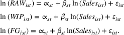
To get a sense of whether such general patterns might be discernible, we first explored our raw data for all listed manufacturing firms with low and high Japan exposure after the GEJE and observed initial counterintuitive corporate responses. On average, firms exposed to Japan appear to have increased raw material inventories (RAW) and volume flexibility in the years following the GEJE (Figure 1a,b). The increase in inventories remained stable over subsequent years, while firms’ volume flexibility weakened again. These initial insights have spurred our interest in whether these patterns can also be observed using more rigorous empirical approaches to investigation. We report on this investigation and its results in this paper.
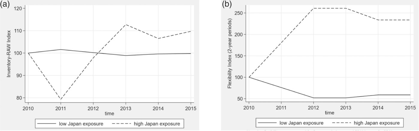
(a) Visual inspection of the changes in raw material inventories (mean values over two groups). The Great East Japan Earthquake occurred on March 11, 2011. (b) Visual inspection of the changes in volume flexibility (measured over 2‐year periods). To estimate volume flexibility, data from two fiscal years needed to be combined (see Section 4). To exclude the distorting effect of 2011, this figure reports values for the periods 2009–2010, 2012–2013, and 2014–2015.
We used a global dataset of 13,797 firms between 2004 and 2017 to gain initial insights into the question: How did firms adjust their inventory levels and flexibility after being exposed to the GEJE? We find, on average, significant RAW increases, temporary flexibility increases, and delayed work‐in‐process (WIP) and finished goods (FG) decreases. These average patterns are more pronounced for risk‐averse firms than for risk‐sensitive firms. In addition, firms appear to have increased inventories more when they already had high inventories prior to the event. In contrast, volume flexibility was increased more in those firms that previously had relatively low flexibility. Our post hoc analyses indicate that Japanese companies experienced a 17.5% to 23.1% decline in return on sales between 2013 and 2017 due to the observed inventory shifts. Based on our results, we discuss what patterns are likely to follow lp‐hc events, consider possible influencing factors, and explain new research priorities that emerge from our observations.
LITERATURE REVIEW
Reacting to supply chain disruptions
This research joins studies that examined stock market responses to firms exposed to disruption risks (Hendricks & Singhal, 2003, 2005). For example, Hendricks et al. (2020) found small but significant losses in shareholder value for firms that experienced supply chain disruptions as a result of the GEJE. The following studies also examined stock market reactions after the GEJE and found similar patterns (Jaussaud et al., 2015; Takao et al., 2013; Tao et al., 2019). In a study of a man‐made event, the Rana Plaza building collapse, Jacobs and Singhal (2017) provide insights into the affected retailers’ stock market losses and short‐lived value losses. These studies suggest investors are concerned about risks and react when events occur, which suggests that firms may feel an obligation to respond. In other words, it is difficult for them to do nothing. In this paper, we document the responses of firms when events occur.
The studies that have examined firms’ structural adjustments in response to risk events have largely relied on case studies and have focused almost exclusively on firms’ reactions during or immediately after the event. Consequently, research has focused on corporate short‐term recovery efforts after lp‐hc events rather than on longer‐term adjustments. For example, Wai and Wongsurawat (2013) highlighted how early detection and quick response benefitted Western Digital's firefighting efforts during the 2011 Chao Phraya River flood in Thailand. Western Digital recognized the failure of its wastewater control systems and moved its own inventory and that of its suppliers to safer locations. Runyan (2006), who spent 3 months interviewing small businesses after Hurricane Katrina in 2005, analyzed the barriers that prevented businesses from recovering quickly, including lack of planning and financial constraints. Sheffi (2005) provides detailed insights on shorter‐term responses to Hurricane Katrina by P&G and other firms. Longer‐term adjustments were considered by Park et al. (2013), who interviewed four Japanese manufacturing firms in depth after the GEJE. All were either directly or indirectly affected by the event, and all reported making immediate investments to restore infrastructure and reestablish communication. For one firm, Park et al. (2013) offer insights into the strategic changes they sought, which included increased inventory of generic components. We add to these anecdotes a large‐scale empirical study examining longer‐term inventory and flexibility patterns of manufacturing firms after the 2011 GEJE.
Inventory, flexibility, and what might drive resilience reactions
Previous operations management research has suggested that two of the most important levers for operational resilience are inventory levels and flexibility (Sheffi & Rice, 2005; Simchi‐Levi et al., 2018). While inventories can temporarily absorb supply disruptions, flexibility is desirable under conditions of uncertainty as well as in normal business operations (Jack & Raturi, 2002, 2003; Koste & Malhotra, 1999). Both levers can be developed ex‐ante or ex‐post to a disruptive event. However, developing flexibility is seen as more economically sustainable, as cost efficiency can suffer when buffering through inventories (Chopra & Sodhi, 2014). Indeed, Eroglu and Hofer (2014) found inventory levels and inventory shortages to be responsible for nearly one‐third of the variation in firm performance.
While prior research has primarily examined whether firms’ responses were economic under certain contextual conditions, the literature is sparse and mostly non‐empirical about longer‐term responses to disruptive events with changes in inventory levels and flexibility. Literature suggests that firms select inventory levels based on probability distributions of customer demand, to maximize expected profit (Eroglu & Hofer, 2014; Lieberman et al., 1999). Using inventory to build resilience has been referred to as “risk mitigation inventory” (Simchi‐Levi et al., 2018). Inventory levels should increase with set‐up costs and decrease with inventory per‐unit costs—keeping other factors such as production schedule instability constant (Metters & Vargas, 1999). Furthermore, the buffering aspect of inventory can be illustrated through varying levels of safety stock (Liu et al., 2016).
Other factors to be considered are the individual inventory components: RAW, WIP, and FG. The components usually receive less individual attention in the literature because the requiresments for these three components are interrelated (Eroglu & Hofer, 2011a). Converting inventories from RAW to WIP to FG essentially means adding value, but it also means losing product flexibility (Goyal & Netessine, 2011). In this regard, holding FG inventory can reduce lead times, but only if the right level of FG inventory is available (Jack & Raturi, 2002). Though, as noted by Stock and Lambert (2001), predicting the right FG inventory level is subject to much more uncertainty than it is for RAW. Our study examines the three types of inventories that firms hold to hedge against disruptions.
Recent disruptive events, for example, the COVID‐19 pandemic, and previous literature on disruptive events have made it clear that the drive for efficiency and inventory reduction has made supply chains more vulnerable (Azadegan et al., 2013; Eroglu & Hofer, 2011b; Knemeyer et al., 2009). Low inventory levels can make firms more vulnerable and more costly (Udenio et al., 2018), which tells us that “too low inventory” is a reality (Eroglu & Hofer, 2011b). To further understand risk aversion and decisions about low inventory‐level setting, we looked at a recent study by Wang and Mersereau (2017), which explored the inventory management concerns of firms in response to lp‐hc events that may (or may not) abruptly change demand patterns. Wang and Mersereau (2017) point out that, following such events, “a manager is torn between using a possibly obsolete demand model estimated from a long data history and using a model estimated from a short, recent history” (p. 341). The authors conclude that managers should generally consider increased uncertainty when a change in demand can be suspected. The findings of Wang and Mersereau (2017) further suggest that risk preference affects how firms respond to such events. We consider firm‐level decisions, but as evident in Wang and Mersereau's (2017) study and discussed in the manager‐firm matching literature (e.g., Bertrand & Schoar, 2003; Bodnar et al., 2019; Graham et al., 2013), much of what is observed in risk behavior and decision‐making at the firm‐level can be used to explain individual‐level behavior.
While classical inventory theory takes most input parameters as given, recent research has shown that many forms of variability are subject to management control (Kremer et al., 2014; Yang et al., 2018). Managers who have already factored high uncertainty into their inventory and flexibility decisions prior to a disruptive event might see their forecast confirmed by the event and decide to maintain the already high levels.
We conclude that forecasting after an lp‐hc event is fraught with complexity and uncertainty, suggesting that managers rely in part on gut feelings and incomplete information. For example, in the immediate aftermath of the GEJE, sales of some products surged, while others declined (Carvalho et al., 2021; Martson, 2011). Were these short‐lived fluctuations or the beginning of longer‐term changes? History shows that in most cases, demand and supply returned to near pre‐event levels relatively quickly, but managers may have had different perceptions of the demand and supply process shortly after the event. These perceptions likely affected the firms’ inventory levels, and decisions regarding the changes in inventories probably consider pre‐event inventory levels. The same is true for a firm's choice of volume flexibility. Volume flexibility allows for quick adjustments in production before, during, and after disruptions (Sheffi & Rice, 2005; Tomlin, 2006). Volume flexibility is sometimes referred to as the strategic response to uncertainty, while inventory buffering is operational (Malhotra & Mackelprang, 2012). Developing volume flexibility is a capability‐enhancing activity that potentially brings lasting competitive advantages to firms (e.g., Malhotra & Mackelprang, 2012; Sawhney, 2006). However, volume flexibility does not come at zero cost, and poorly considered investments in flexibility could be detrimental (Narasimhan et al., 2004).
Common strategies for increasing volume flexibility include the use of overtime, temporary workers, cross‐training workers, or developing complementary product portfolios, layout, inventory buffers, and outsourcing, to name a few (Jack & Raturi, 2002). Thus, inventories and flexibility are not opposing or mutually exclusive strategies. However, more flexibility is associated with a relatively small increase in operating costs, overcoming the initial cost‐flexibility tradeoff. A firm that uses more inventory to increase service levels is generally not more flexible because an increase in inventory costs reduces economic efficiency in managing variability. Therefore, firms usually face a tradeoff and are likely to choose a combination of the two.
We will examine general patterns of inventory and volume flexibility following the GEJE. Building on our literature review, we also examine whether the expression of such patterns can be partially explained by firms' risk aversion. Linking response patterns to firms' risk aversion would improve our understanding of the complexity and uncertainty that firms face in making such decisions. Finally, we also investigate whether the patterns can be partially explained by the availability of inventories and volume flexibility before the event. Findings in this direction would help us develop an initial understanding of some of the mechanisms that may have guided firms in their decisions.
SAMPLE AND DATA SOURCE
The empirical goal was to see if the general patterns observed would stand up to closer scrutiny and if we could gain further insights. Causality, in this context, can be demonstrated only by abundant consistent evidence. Therefore, future complementary research will be needed to provide more certainty in this direction. In the following sections, we explain the stepwise approach we took to examine the data in a variety of ways to remove noise and tease out patterns.
We collected secondary data from around the world for all listed manufacturing firms (North American Industry Classification System [NAICS] 31–33) on Datastream, for 14 consecutive years (2004–2017). This resulted in an unbalanced panel of 13,797 firms and 164,443 firm‐year observations. Sample distribution of the nationality of the firms is available in the Supporting Information, Section 1.
When preparing the data, uniform annual intervals were defined for all countries and firms. Since the definition of a fiscal year (FY) varies between and within countries (and sometimes even within firms), we defined consistent annual intervals according to the end dates of each firm's reporting periods in each FY. The consistent annual intervals were aligned with the GEJE date (March 11, 2011). Because the end dates of the reporting periods are usually at the beginning or end of the month (e.g., Japan's FY 2010 ended on March 31, 2011), the 2010 interval includes all FY observations whose reporting period ended between March 2, 2010, and March 1, 2011; Japanese firms’ reports released on March 31, 2011, (i.e., after the event) were included in the 2011 interval. A visual representation of this process can be found in the Supporting Information, Section 2.
In addition, for a small number of firms, reporting period end dates were not reported in Datastream for all consecutive FYs, even though all other firm data were available. Only in cases where the day and month of the reporting period end date of two reporting periods in the previous and subsequent FYs were identical, did we determine the missing period end dates using the corresponding reporting period end date for that missing period. In this way, we recovered an additional 7,732 firm‐year observations—the results of the estimation without these additional observations are reported in the Supporting Information, Section 10. The results remain qualitatively unchanged.
Extreme values were excluded from the analyses to avoid the risk of bias due to outliers and potentially incorrect data entry (Wooldridge, 2016, pp. 296–300). Specifically, 1% of the lowest records in all four risk measures we used were omitted. This resulted in the exclusion of about 2.4% of the firm‐year observations. The results of the estimation including extreme values are reported in the Supporting Information, Section 10. The results remain qualitatively unchanged.
MEASURES
To operationalize inventory (Inv) levels that allow for a meaningful comparison over time, we estimated the negative of the empirical leanness indicator (ELI) as proposed by Eroglu and Hofer (2011a). The ELI relies on inventory turnover curves
1
but also considers economies of scale and represents the non‐linear relationship between inventories and firm size. Specifically, ELI accounts for time‐related changes specific to the respective industry sector. This allows for better comparability of a firm's inventory levels over longer periods. In short, ELI represents a firm's inventory levels relative to the time and competitors. To estimate ELI, the natural logarithm of a firm's average inventory (in USD) was computed for each inventory type in year t (Equation 1).
2
∝ is the industry‐specific intercept in year t; ln(Salesist
) is the natural logarithm of the net annual sales volume of firm i in industry sector s using four‐digit NAICS codes and year t. We then obtained the firm's Invx
value (for inventory type x [x = RAW, WIP, FG] denoted as Invx
) by taking the corresponding studentized residuals

To assess volume flexibility (VF), we followed Jack and Raturi's (2003) operationalization of volume flexibility as defined in Koste and Malhotra (1999). The authors considered two process variables to assess a firm's volume flexibility: fluctuations in inventories and fluctuations in production costs. They argue that variations in inventories over time and variations in production costs must be benchmarked to variations in sales because a firm facing high demand uncertainty needs larger buffers and faces higher production costs. Thus, a firm that can respond to larger sales variations with smaller inventory variations and production costs (as measured by the cost of revenue) is considered to have more volume flexibility. Consequently, VF was assessed considering inventory and production technology tradeoffs (Equation 2).
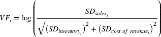
A higher number indicates greater volume flexibility. We assessed VF twice, employing 2‐year and 3‐year lagged data, accounting for the tradeoff between measurement precision and fluctuations in a firm's VF over time. That is, VF with 2‐year lagged data used inventory and cost of revenue in t and t‐1 to calculate SDinventory and SDcost of revenue , while t, t‐1, and t‐2 were used to calculate VF with 3‐year lagged data. Since the flexibility measure includes repeated observations for all firms, we adjusted standard errors for clusters at the firm level. Note that VF considers the standard deviation of total inventories, which is different from what we used to measure Invx . To account for the tradeoff in measurement accuracy and potential changes of a firm's VF over time, we will estimate VF using 2 years and 3 years of lagged data in our exploration.
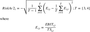
To assess firms’ risk‐averse behavior (RiskAv) in investment decisions, we employed two measures as proposed by John et al. (2008) and Boubakri et al. (2013). The proxy in John et al. (2008) assesses the degree of risk aversion in firms’ investment decisions based on the volatility of corporate earnings over multiple years as (i) the market‐adjusted volatility of firm‐level earnings over a certain period, (ii) the country average of the volatility of firms’ earnings, and (iii) an imputed country risk score based on industry risk characteristics. The assumption is that riskier corporate investments have more volatile returns to capital. For each firm with available earnings and total assets, we computed the deviation of the firm's EBITDA to total assets ratio from the country average for the corresponding year. A firm's pre‐event risk‐averse behavior was then defined as the negative standard deviation of this country‐demeaned ratio of EBITDA to total assets over a 3‐ or 4‐year period T (Equation 3). A higher number indicates risk aversion, while a lower number indicates risk‐seeking. For a more in‐depth discussion of the measure and empirical proof, we recommend John et al. (2008).
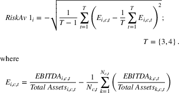
Nc,t indexes the firms in country c in year t. Index i is used for the firm. The measure is based on the relative variation in firms’ financial performance and, thus, is a proxy for firms’ actual behavior.
Acknowledging that many publicly listed firms work across industries and countries, we also assessed risk aversion through the measure proposed by Boubakri et al. (2013). This measure considers the volatility of the ratio of EBIT to total sales over multiple years. This approach mitigates our concern that total assets are sensitive to inflation, accounting conventions, and management concerns because it involves the flow measures of EBIT and sales (Equation 4).
EBITi,t is defined as the earnings before interest and taxes of firm i in year t, and TSi,t is equal to the corresponding total sales. We again evaluated the measure using 3‐ and 4‐year (T) lagged data. Although Boubakri et al. (2013) assessed the risk measure using just 4 years of data, for robustness and to allow for an overlap with the assessment of VF, we estimated RiskAv1 and RiskAv2 with 4‐ and 3‐year lagged pre‐event data. While we would have explored the effect of a firm's risk preference after the catastrophe, such attitudes are likely influenced by the event and could have confounded our analyses. In contrast, the pre‐event risk‐averse behavior, as assessed by the two risk measures, is exogenous to the event. The means, standard deviations, and correlations of the main variables are reported in Table 1.
Means, standard deviations, and correlations of key measures
Note: The ELIRAW ‐baseline specification sample was used for this table. “D” represents the treatment variable in the baseline specification, where D = 1 if a firm's risk country metric indicates the highest risk value for Japan.
***, **, and * indicate significance at the 0.01, 0.05, and 0.10 levels.
We used the firm‐specific “country‐of‐risk” metric offered by Datastream as a proxy for the treatment variable. This metric allows us to approximate whether a firm was (or was not) exposed to the GEJE without having to use an attribution mechanism, the impartiality of which we would have difficulty trusting (Titiunik, 2021).
The country‐of‐risk metric was developed by Refinitiv, a provider of risk assessment tools and financial data, and is available in Datastream. The metric quantifies a firm's exposure risk to a country and ranges from 0 to 1. 3 The value is based on a combination of analytics and algorithms developed by Refinitiv and is based on the following factors: sales, headquarters, country in which its primary stock is traded, and financial reporting currency. The resulting value is a country‐specific weight that indicates the firm's country‐specific exposure relative to all other countries in which it operates (Refinitiv, 2021).
Next, we examined how well this metric can be used to reflect a firm's operational engagement in Japan in 2010 (before the earthquake). For this purpose, we took advantage of the fact that many Japanese firms published their share of assets, production output, employees or/and properties/plant/equipment in Japan, compared to the rest of the world for 2010. We manually collected this information from the Bloomberg Markets database for a random sample of 435 Japanese firms. We selected Japanese firms for the analysis because firms outside Japan generally do not disclose their exposure to Japan. The obtained descriptive sample statistics on the share of assets, production output, employees, and properties/plant/equipment in Japan in 2010 are shown in Table 2. We then performed a t‐test for equality of means for the proportion of assets between the two groups. The test was rejected with a t‐value of 18.4. Pearson's correlation coefficient between the proportion of assets in Japan and group identification is 0.71 (p < 0.01). The Spearman rank correlation is 0.77 (p < 0.01). Because we lack observations for the other three metrics, we could not meaningfully examine them for group differences by t‐tests. Yet, because the risk country score is a continuous variable, we were able to estimate correlations for two of these scores. Still, in interpreting the results, we caution that the correlation values obtained are mainly based on variation in the high‐risk group (above 0.9), which could give a somewhat biased picture. Nevertheless, we obtained a Pearson correlation coefficient of 0.98 (p < 0.01) for the percentage of production in Japan in 2010 and the risk country value for Japan. Similarly, the Pearson correlation coefficient between the percentage of employees in Japan in 2010 and the risk country score is 0.76 (p < 0.01). We lack sufficient data to reasonably examine the correlation coefficient between the percentage of tangible assets in Japan in 2010 and the country‐at‐risk score, so our interpretation of the association of this operational metric with the country‐at‐risk score is based on the descriptive statistics in Table 2. In summary, we interpret the results obtained as providing strong evidence of a significant and substantial association between the country‐of‐risk score for a firm and that firm's operational exposure to Japan. Further information on the process is available in the Supporting Information, Section 3.
Descriptive statistics for the association between the country‐of‐risk metric and firms’ share of assets, production output, employees, and property/plant/equipment using the example of Japan (N = 435)
Nevertheless, the country‐of‐risk value remains a proxy to determine “exposure,” as it seems reasonable to assume that not all firms in the treatment (control) group were affected (unaffected) by the 2011 disaster. Thus, while our analyses show a strong association of the value with a firm's operational exposure to Japan in 2010, we were unable to examine whether it also considers the risk that a firm's supply chain was exposed (or not exposed) to the event. Extreme cases could be a firm in Japan that sources exclusively from abroad, or a firm that has no factories in Japan but whose supply chain originates exclusively from Japan. The most likely implication of these considerations is that the coefficients estimated in the following underestimate the underlying effect associated with the GEJE. This follows from the assumption that not all firms in Japan were affected by GEJE, and/or some firms in the control group were indirectly affected through their supply chains. Both resulting biases would move the estimated patterns toward zero (for a more detailed discussion and explanation, see Section 4 of the Supporting Information). In other words, the drawback of the country‐of‐risk metric is that the real effects were likely stronger than what we estimated.
DATA EXPLORATION
Exploration approach 1: The baseline specification
We began our analysis with a baseline specification, where firms with the highest country risk value for Japan were defined as the treatment group. Firms for which the highest country risk value was not Japan were included in the control group (except for firms with the highest risk in Thailand, which was hit by a major flood in the summer of 2011; the estimation results including Thai firms in the treatment group are shown in the Supporting Information, Section 10; the results remain qualitatively stable with this decision). Because of the nature of the event, we refrained from creating a control group based on spatial proximity to Japan as such regions were likely impacted by the event. However, we later examined the cultural differences between the two groups and their effects on the observed patterns, and the results did not raise concerns—see exploration approach 4. Similarly, it would have been difficult to define the approximate treatment and control groups across industries because there are few manufacturing industries that are not represented in Japan. Consequently, an approximation of the treatment by the country risk value of Japan appears to be an appropriate approach.
Model specification
To estimate the coefficients of interest, we used a common approach to identify the average treatment effect on the treated (ATT). The difference in difference (DID) estimation allows firms in the treatment and control groups of the natural experiment to arbitrarily differ before the event (Lechner, 2011, p. 189). Using such a causal method allows us to attribute the observed patterns to the GEJE with greater certainty, but without arguing for causality, as this would require further evidence. Please consider Equation (5), which was estimated after applying the within transformation: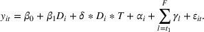
The effect of being in the treatment group is represented by β1. 

To explore inventory patterns after the GEJE, we used the pre‐treatment period from 2009 to 2010. We used the post‐treatment period of 2013 to 2015 to estimate changes while removing all firm‐level, time‐constant confounders. By restricting the ATT to a constant from 2013 to 2015, we maximized efficiency (Lechner, 2011, p. 213; Wooldridge, 2010, p. 151) and minimized measurement error linked to the approximative nature of Invx . As the Invx for 2012 is calculated using the total inventory dollar values from FY2011 and FY2012, the first post‐disaster Invx that is free of the immediate impact of the event was 2013. Hence, in every step of the analysis, we omitted the treatment year immediately after the event, to exclude the unavoidable immediate effect of the catastrophe on inventory levels from the results. The results with inclusion of the crisis years are presented in Supporting Information, Section 11.
To explore volume flexibility after the GEJE, we left out FY 2011 to ignore the immediate and expected volatility induced by the event. VF 2 yrs was measured over non‐overlapping 2‐year periods, comparing the pre‐treatment period 2009 to 2010 with two post‐treatment periods 2012 to 2013 and 2014 to 2015. VF 3 yrs considers the pre‐treatment period 2008 to 2010 and the two post‐treatment periods 2012 to 2014 and 2015 to 2017.
Next, to explore the effect of corporate risk aversion, we again conducted a DID estimation. For the analysis, corporate risk‐averse behavior was included as an interaction term with ATT in the DID estimation (Equation 6). The key variable of interest is the coefficient θ of the interaction term. The effect of time‐invariant variables 


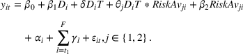
Finally, to identify firm reactions based on their pre‐event availability of inventory buffers and volume flexibility, we used a triple‐differencing specification, a regression representing differences‐in‐differences‐in‐differences (DDD; Equation 7). We estimated Equation (7) on the data from 2009 to 2015, where 2011 to 2012 and 2011 were left out with the specification with Invx
and VF, respectively. The equation for flexibility thusly involved further interaction terms with the 2012 dummy. In Equation (7), d2014 represents the dummy variable for the year 2014, “High” represents a group having high inventory/flexibility, D represents the treatment group, and T equals one for all periods after the earthquake (2013 to 2015 for Inv and 2012 to 2015 for VF).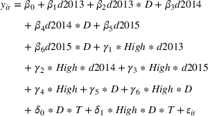
While the DID estimate allows us to compare the different reactions in the approximative treatment and comparison groups after the GEJE, the triple difference estimator helps uncover the difference in reaction between high‐ and low‐Invx/VF firms in the treatment group relative to the difference in reaction of high‐ and low‐Invx/VF firms in the control group. The coefficient of interest is given by δ1, which is better illustrated by Equation (8). Equation (8) illustrates the DDD estimator in terms of differences between group means of the dependent variable y. Let t‐1 denote the pre‐treatment and t + 1 the post‐treatment period; subscripts D and C represent the approximative treatment and control groups, respectively. Meanwhile, high and low subscripts represent firms with either high‐ or low‐volume Invx/VF in the pre‐treatment period. For our main specification, we deemed a firm as having high‐Invx
or high‐VF if its average inventory buffers or average volume flexibility in the considered period is higher than the median in the period before the earthquake (i.e., 2009–2010; estimation results for mean, 25th and 75th percentile as alternative thresholds are reported in the Supporting Information, Section 10. The results remain qualitatively unchanged.)
There are some further assumptions invoked by the DID approach (Lechner, 2011, pp. 176–182). First, the method necessitates that the difference between the two groups would have stayed the same had the event not occurred. We tested this key identifying assumption by using a placebo treatment over a period in which we believed no major event occurred. The year 2006 was chosen for this test because the placebo event had to occur before 2008 (the year of the financial crisis)—as can be seen from our FY definition, the 2008 financial crisis affected Japanese and Western firms at different times. Due to the construction of the VF measure and the availability of the data from 2004 onward, we could perform placebo tests only in the pre‐treatment period for VF 2 yrs . For Invx and VF, we could not reject the null hypothesis of no effect in 2006, supporting the identifying assumption that the treatment and control groups experienced similar development in inventory and flexibility prior to the catastrophe (see Table 3).
Regression estimates of a 2006 placebo event experience on inventories and flexibility: Baseline specification
Note: t‐values in parentheses. Invx : pre‐treatment period 2005, post‐treatment period 2007. VF 2 yrs : pre‐treatment period 2004–2005, post‐treatment period 2007–2008. Note that each model considers all data available in the unbalanced panel. The number of observations vary from model to model because not all firms reported on all dependent variables and years and because the dependent variables take into account different lagged periods.
***, **, and * indicate significance at the 0.01, 0.05, and 0.10 levels.
Another placebo treatment was administered after the event. The year 2015 was chosen, with 2013 to 2014 4 serving as the pre‐treatment and 2016 to 2017 as the post‐treatment. Table 4 summarizes the results of this test. It is important to note that the violation of the common trend after the event would not challenge its validity before the event. The results are interesting because the observed adjustments, as they suggest with respect to inventory levels, are more likely due to the GEJE than coincidental, as the trends in the two groups neither diverge further nor revert to the origin after 2015. Thus, this test restricts the set of plausible alternative explanations for the observed patterns with respect to the inventory adjustments. Pre‐empting the observed patterns with respect to flexibility, the results of the post‐event placebo test suggest a reversion of the flexibility level increases toward the pre‐treatment levels after the event. This is a cautious indication that the post‐event increase in flexibility may have been short‐lived. Furthermore, the negative estimates of the placebo test in 2015 make potential alternative explanations for the significant positive findings after the GEJE (e.g., diverging pre‐event trends in the control and treatment groups) less plausible. Unfortunately, the financial crises in 2008 splits the pre‐treatment period and renders impossible a more conclusive test of the parallel trend assumptions, which is why we are cautious about interpreting our results causally.
Regression estimates of a 2015 placebo event experience on inventories and flexibility: Baseline specification
Note: t‐values in parentheses. Invx : pre‐treatment period 2014 (2013–2014 for InwRAW ), post‐treatment period 2016–2017. VF 2 yrs : pre‐treatment period 2013–2014, post‐treatment period 2016–2017. Note that each model considers all data available in the unbalanced panel. The number of observations vary from model to model because not all firms reported on all dependent variables and years and because the dependent variables take into account different lagged periods.
***, **, and * indicate significance at the 0.01, 0.05, and 0.10 levels.
This study favors the plausibility of the common trend assumption inherent in the DID approach over the unconfoundedness assumption in matching‐only techniques. Matching requires the unconfoundedness assumption, which postulates that the control group—after matching—produces, on average, a valid estimate of what would have happened to Japanese firms if the earthquake had not occurred. This means that there must be no unobservable differences between the treatment and control groups after matching the observed characteristics. This is equivalent to assuming that we can observe any factor that affects the firm's exposure to the event (treatment) and its potential outcomes with and without the event. The potential outcome in our case is firms’ inventories/flexibility after the GEJE and firms’ inventories/flexibility had the GEJE never occurred. We cannot define characteristics that would make this assumption plausible. Another problem is that the unconfoundedness assumption cannot be tested. In contrast, the DID approach allows for differences between the treatment and control groups, even if they are due to unobservable characteristics (Lechner, 2011, p. 189) if they remain constant over the observation period (i.e., the common trend assumption). For this reason, we combined a sample adjusted for observed characteristics with the DID and DDD approaches while looking for significant changes in estimates to test whether structural differences between the treatment and the control groups can explain the observed patterns. We did not condition the value of the explanatory variable before treatment in our DID approach because conditioning on the value of inventory or flexibility before the GEJE should make the resulting identification more plausible. However, Lechner (2011, p. 192) points out that holding the pre‐treatment part of this difference constant (by conditioning on the pre‐treatment outcome variables at the individual level) is equivalent to focusing on just the post‐treatment variables alone. Thus, conditioning on the pre‐treatment variables in the DID framework would be equivalent to assuming the unconfoundedness (the matching) assumption.
Another assumption of the DID approach is that the pre‐disaster levels of the outcome variables should not be influenced by the event. This is fulfilled by design since the GEJE could not have been anticipated on any reasonable time scale.
Observed general pattern and alternative explanation
Table 5 reports the coefficients for the baseline specification.
Regression estimates of the Great East Japan Earthquake (GEJE) event experience on inventories and flexibility: Baseline specification
Note: t‐values in parentheses. Invx : pre‐treatment period 2009–2010, post‐treatment period 2013–2015. VF 2 yrs : pre‐treatment period 2009–2010, post‐treatment period 2012–2015. VF 3 yrs : pre‐treatment period 2008–2010, post‐treatment period 2012–2017. Note that each model considers all data available in the unbalanced panel. The number of observations vary from model to model because not all firms reported on all dependent variables and years and because the dependent variables take into account different lagged periods.
***, **, and * indicate significance at the 0.01, 0.05, and 0.10 levels.
We observe a significant increase in InvRAW in the post‐event period (2013 to 2015). The observed increase is estimated to be 0.083. This can be interpreted as a 3.3% move along the InvRAW distribution. The InvRAW increase remains highly significant when estimated for each post‐treatment year separately (see Supporting Information, Section 5). The results also point to a significant pattern in InvWIP , with a coefficient of −0.049, suggesting a reduction in WIP inventories. Annual analyses reveal that firms reduced InvWIP with a one‐year lag to the observed increase in InvRAW (see Supporting Information, Section 5). Similarly, we identified a 1‐year lagged significant reduction in InvFG with a coefficient of −0.054 over the observed post‐event period.
We find similar evidence for an overall increase in volume flexibility in the treatment group. Assuming a normal distribution, we find that the adjustments in VF 2 yrs signify a 9.6% move. These patterns are found to be robust against variations in sample specification and data handling (see Supporting Information, Section 10).
To further investigate our observations, we explored whether the identified adjustments can partly be explained by firms shifting their production away from Japan. We studied this possibility by examining the stability of the share of assets that Japanese firms held in Japan, comparing pre‐ and post‐event data. Specifically, we find that 63% of the firms in our sample (for sample description, see Supporting Information, Section 3) reported no changes between 2010 and 2017. Overall, the observed mean difference indicates a non‐significant (p = 0.842) increase by 1.7% in firms’ share of assets in Japan after the event. We conclude that the percentage of total assets in Japan remained relatively stable from before the event until the end of the observation period. This is noteworthy as it provides some indication that the observed inventory patterns did not significantly shift the geography of asset holdings in affected firms or can be interpreted as a result thereof.
Patterns in relation to pre‐event risk preferences
Next, we set out to explore the relation between pre‐event risk preferences and inventory and flexibility patterns after the event. The results are reported in Table 6.
Regression estimates of the GEJE event experience on inventories and flexibility relative to pre‐event risk‐averse behavior: Baseline specification
Note: t‐values in parentheses. Invx : pre‐treatment period 2009–2010, post‐treatment period 2013–2015. VF 2 yrs : pre‐treatment period 2009–2010, post‐treatment period 2012–2015. VF 3 yrs : Pre‐treatment period 2008–2010, post‐treatment period 2012–2017. RiskAvX 3 yrs : 2008–2010. RiskAvX 4 yrs : 2007–2010. Note that each model considers all data available in the unbalanced panel. The number of observations vary from model to model because not all firms reported on all dependent variables and years and because the dependent variables take into account different lagged periods.
***, **, and * indicate significance at the 0.01, 0.05, and 0.10 levels.
Table 6 presents evidence for an amplified InvRAW and VF coefficient in risk‐averse firms. The observed θ for 2013, 2014, and 2015 with respect to InvRAW indicate that a moderate increase/decrease in risk aversion of a firm already determines whether a firm acted or not. To illustrate this, we computed the degree of risk aversion required to observe no pattern. For InvRAW , we observed that for firms assigned to the treatment group in 2013, 2014, and 2015, it would have taken a decrease of only 14% to 33% (RiskAv13 yrs ) or 1% to 3% (RiskAv14 yrs ) along the sample standard deviation to observe no changes. For the RiskAv2, it would have taken 38% to 92% (RiskAv23 yrs ) and 35% to 82% (RiskAv24 yrs ) of the sample standard deviation to cancel InvRAW changes. Similarly, the results suggest that if an average firm was 40% of a standard deviation less risk‐averse, taking the RiskAv24 yrs measure would not result in flexibility changes. We conclude that if the average firm was one standard deviation less risk‐averse, it would not have changed its InvRAW or VF. Further, we find little to no evidence for changes in InvWIP and InvFG to be dependent on firms’ risk preference, given that the only significant change of InvWIP was detected when estimated with RiskAv2. This suggests that InvWIP and InvFG changes, as opposed to InvRAW and VF, can to a very small extent be explained by organizational risk aversion. These patterns are also found to be robust against variations in sample specification and data handling (see Supporting Information, Section 10).
Patterns in relation to pre‐event availability of inventory and volume flexibility
Next, we explored whether the observed patterns are related to firms’ pre‐event availability of inventory and volume flexibility. The results are summarized in Table 7 (the complete set of estimated coefficients of Equation 7 are reported in the Supporting Information, Section 6).
Moderating effect of pre‐event inventory/flexibility on inventory/flexibility changes: Baseline specification
Note: t‐values in parentheses. Invx : pre‐treatment period 2009–2010, post‐treatment period 2013–2015. VF 2 yrs : pre‐treatment period 2009–2010, post‐treatment period 2012–2015. VF 3 yrs : pre‐treatment period 2008–2010, post‐treatment period 2012–2017. Note that each model considers all data available in the unbalanced panel. The number of observations vary from model to model because not all firms reported on all dependent variables and years and because the dependent variables take into account different lagged periods.
***, **, and * indicate significance at the 0.01, 0.05, and 0.10 levels.
We find that firms with high inventory buffers before the event have added significantly more inventory after the GEJE vis‐à‐vis firms with low pre‐event inventory buffers. This holds true for InvRAW and InvFG . However, this does not hold true for the InvWIP . The test also provides consistent evidence for an opposing reaction with respect to VF. Firms with low pre‐event flexibility have increased volume flexibility more strongly than firms with high pre‐event volume flexibility. These patterns appear robust against the use of alternative thresholds to define “high” and “low” pre‐event resources, as well as against changes in sample specification and data handling (see Supporting Information, Section 10).
Exploration approach 2: Propensity score matching (PSM)
Exploration approach 1 could control for only time‐constant effects. Therefore, in the next step, we enhanced our approach by adding PSM to explore whether the results were driven by observed differences in our control and treatment groups. The model specification and observed patterns are reported in the Supporting Information, Section 7.
Overall, these results indicate that the results presented in exploration approach 1 are not likely to be a mere consequence of the limited comparability of the treatment and control group with respect to the observed characteristics. We find that even if less than 30% of the original sample is used to enhance the comparability between the treatment and control groups, the main results do not change significantly at the 5% level.
Exploration approach 3: The restricted‐groups specification
Exploration approach 2 helped us to develop a better understanding of whether the observed patterns were driven by structural differences of firms in the control and treatment groups. However, concerns remained that our approach of categorizing firms into treatment and control groups reported in exploration approach 1 might have been too simplistic. In extreme cases, it could have happened that an exceptionally geographically dispersed firm with a country‐of‐risk metric for Japan of 0.3 was selected into the treatment group because of its exposure to several other countries, while a firm with a country‐of‐risk metric for Japan of 0.4 might be in the control group, while it was only exposed to two countries. Therefore, in the next step, we developed a stricter approach to defining the two groups. We denote this as the restricted‐groups specification.
For our main specification, we chose the treated group to include any firm with a Japan‐specific weighting higher than 0.5. The control group is populated by firms with exposure to Japan that is less than 0.05. In addition, we also employed another, likewise arbitrary, threshold of 0.67 for the treated groups and 0.10 for the control groups. The two approaches came again at the expense of sample size (approximately 50% smaller) vis‐à‐vis exploration approach 1. Further details on model specification and observed patterns are reported in the Supporting Information, Section 8. The results remain qualitatively consistent across specifications and when compared to the results of exploration approach 1.
Exploration approach 4: The weighted baseline and restricted groups specification
Finally, we explored whether the observed patterns may be a testimony to the cultural differences between the groups. For this, we made use of the widely known and applied conceptualization of national culture by Hofstede et al. (1990) and weighted the baseline and restricted groups specification for cultural differences between the firms in the sample. For our main specification, we considered the differences in all six culture dimensions. Thereafter, we likewise weighted and estimated all models only considering Hofstede's “uncertainty avoidance” dimension, as it may be more closely related to firms’ risk behavior. Details on model specification and observed patterns are reported in the Supporting Information, Section 9. Neither approach to weighting groups by cultural differences changes the picture of the patterns uncovered in exploration approach 1. The results remain qualitatively unchanged.
EVENT SELECTION AND THE LEVEL OF ANALYSIS
We chose the GEJE because, despite its devastating societal impact, it did not depend on the characteristics of firms and managers, the location of the event was relatively well‐defined, and the years following the event were not characterized by other similarly destructive events. This means that we cannot simply attribute the observed patterns in corporate policy after the event to reverse causality or unobserved heterogeneity, and it is therefore possible for us to view and study the GEJE in large part as a quasi‐natural experiment.
For our study, we had to define a level of analysis as well as the treatment and control groups. In an ideal experimental design with clearly defined treatment, firms would have to be randomly assigned to exposure to the GEJE or not. All firms in the sample would operate a single factory, have no supply lines, and produce only final products. Even in such a simplified framework, it would be difficult to determine the true magnitude of the effect. For example, one could measure the distance to the epicenter of the earthquake as a proxy for the intensity with which the firm was affected—but the GEJE affected firms in so many ways that distance to the epicenter alone cannot adequately explain how severely a firm was affected. Some nearby firms suffered structural damage, while others farther away were exposed to indirect but severe technological accidents or suffered supply and transportation disruptions. In one example, following damage to the Fukushima Daiichi nuclear power plant, the Japanese government temporarily shut down all nuclear reactors. In addition, refinery fires and shutdowns in Kashima, Negishi, Sendai, and Tokyo Bay, as well as a series of outages at petrochemical plants, resulted in a short‐term loss of more than 30% of the country's refining capacity and 25% of its ethylene production capacity (Krausmann & Cruz, 2013), prolonging power outages and fuel supply shortages. The power rationing extended from the northeast coast to 200 km south of Tokyo. Four days after the event, the BBC reported that fuel was unavailable at nearly all gas stations in the country, and stores ran out of basic foods and bottled water (Martson, 2011). All Japanese ports were briefly closed. Not only do these events show that distance from the epicenter is difficult to use as an instrument, but they also raise the question about the level of analysis: firm versus factory and country versus regional. Both firm‐level and factory‐level analyses would be subject to bias from omitted variables related to the position and importance of the factory in the internal supply chain. Firms that operate multiple factories are likely to invest more resources in a shorter recovery period for factories that produce critical components. Any long‐term adjustment to a factory's inventory and/or flexibility would likely correlate with the same criteria of importance (i.e., relevance to internal supply chain/production, profit margin, etc.). Similarly, a factory located far from the epicenter might not be able to resume production because of the geographic spread of the impacts.
While the firm‐level analysis would suffer from omitted variable bias, we have found two distinct advantages of analyzing at the firm level. First, intra‐firm dependencies in the supply chain are automatically considered. Second, because of the availability of secondary data, firm‐level analyses are feasible on a much larger scale and are not hampered by unquantifiable selection and response biases as would occur with factory surveys. If we agree on the feasibility of firm‐level rather than factory‐level data, the country seems to be the appropriate level at which to divide firms into treatment and control groups since firms operate multiple factories within and sometimes outside the country, and the most detailed reporting of secondary firm data is usually done at the country level.
DISCUSSION
Our research provides initial insights into how affected manufacturing firms changed their levels of inventory and volume flexibility after the GEJE. Affected firms appear to have increased their inventory levels and, for a shorter period, their volume flexibility – this conclusion is based on the results of our placebo tests after the event. More detailed explorations into inventory adjustments show an immediate increase in RAW inventories, while WIP and FG inventories were reduced after the event with a 1‐year lag. In addition, we find that firms’ risk aversion and the availability of inventory and flexibility prior to the event altered the strength of the observed patterns. Risk‐averse firms were found to have significantly larger increases in RAW inventories after the GEJE than risk‐seeking firms. An increased buildup of inventories was also noted in firms that had relatively high RAW and FG inventories prior to the event. In contrast, firms that had greater volume flexibility before the event appear to have reduced it to a relatively greater extent after the GEJE.
We expect that the present research findings will not necessarily provide answers but rather lead to a new set of research questions. In what follows, we select three findings that we consider particularly noteworthy and discuss potential future research.
Economic implications
The results regarding the increase in RAW inventories and the decrease in WIP and FG inventories raise the question of the possible economic consequences of such reactions. From an empirical perspective, we performed post hoc analyses and found evidence that the inventory shifts identified between 2013 and 2015 reduced the affected firm's return on sales by between 17.5% and 23.1% (see post hoc analysis in Supporting Information, Section 12).
Furthermore, based on our interpretation of the relevant literature, the observation of a longer‐term increase in RAW inventories came unexpectedly. Academics are admittedly cautious about recommending preparedness for lp‐hc events. Nevertheless, it is generally concluded that the development of long‐term inventory buffers is economically impractical—as may be supported by our post hoc analysis. The literature suggests that in many cases, no response or contingency tactics, such as rerouting, that is, increasing production at alternative suppliers/locations or switching transportation modes, or demand management by shifting customer demand to available products, are likely to be more economical responses than inventory buffering (Sheffi & Rice, 2005; Tomlin, 2006). Similarly, the literature has also looked at supplier diversification in the face of uncertainty (Anupindi & Akella, 1993; Tomlin & Wang, 2005). Accordingly, our expectation was that rare events such as the GEJE would not require longer‐term adjustments in inventories; if anything, the event should cause changes in flexibility or lead to the development of longer‐term contingency strategies. While our results indicate that inventory shifts likely reduced financial performance, this analysis does not account for the long‐term benefits of this strategy in the event of a recurrence. To date, there is little evidence in the literature on when inventory tactics are superior to flexibility tactics, considering event characteristics such as probability and impact. Important insights in this direction were provided by Simchi‐Levi et al. (2018), but more is needed in terms of event properties and inventory types to include the impact of inventory shifts. Firms typically do not make decisions at the level of the total inventories, but they decide on RAW, FG, and maybe even on WIP. Such empirical insights are lacking and could, for example, be addressed through optimization models.
In other words, increasing resilience after an incident may make sense in certain cases, namely, when firms use the event as an opportunity to learn and improve (Choi et al., 2020). It is possible that only when firms experience the negative impact of disruptions, do they realize their vulnerability and take corrective action. Such actions may include improving a firm's ability to persist and adapt and making transformational changes to its business model. Such considerations are consistent with recent conceptual thinking in our field that discusses the adaptive side of risk management (Craighead et al., 2020; Wieland & Durach, 2021), a largely unexplored field. Determining how much of the observed patterns are due to firms trying to become more robust and how much is a testament to firms changing in the face of lp‐hc events is an important topic that would also benefit from additional research.
In this vein, and somewhat following the bullwhip logic, it could be assumed that RAW increases after the GEJE could partly be the result of a rippling effect in the supply chain. In the aftermath of the GEJE, firms faced delayed order fulfillment and logistical issues that affect the flow of incoming goods. However, it is reasonable to assume that this effect should have subsided over the years. Indeed, it can be observed that the annual estimates shown in Supporting Information Table 2 fluctuate, suggesting a somewhat lower RAW level for 2015 than for 2013, while the post‐event placebo tests show no significant changes after 2015. Along these lines, it would also be interesting to study the patterns and timing of ripple effects in supply chains following lp‐hc events, possibly through simulations. Such insights could serve two purposes: First, managers would better understand when to expect normal operations to resume. Second, researchers could use such insights to develop their normative recommendations for when to apply which mitigation strategy.
Behavioral causes
The preceding considerations are largely aimed at interpreting our results under the assumption that managers (want to) make exclusively rational decisions, even though, as argued in the literature section, the problem they face is difficult, and therefore managers must rely in part on incomplete information to make decisions. In other words, it is likely that managers do not conduct a fully informed cost‐benefit analysis after an lp‐hc event before deciding whether and how to adjust resilience. Thus, the assumption of rationality is likely to be flawed. Our observation that the patterns appear to be driven by factors such as risk aversion and resource availability prior to the event seems to support this assumption. In addition, the timing and duration of the observed changes—delayed decline in WIP and FG inventories and temporary increase in flexibility—are interesting, as they suggest that the affected firms made not only a one‐time adjustment decision but also began some kind of search for a new operational equilibrium after the event.
Interestingly, problemistic search theory, used to describe organizational search behavior in response to performance‐inhibiting experiences, proposes that the resources available prior to an event can explain how firms search for factors that need to be adjusted after an event (Posen et al., 2017). The theory suggests that finding factors to increase resilience and implementing them is likely to be limited by “we've always done it that way” thinking (Cyert & March, 1992). There are several arguments that support such a theory. First, formerly used approaches to solving a problem tend to provide a higher level of familiarity for decision‐makers (Jung & Lee, 2015) and tend to be more closely associated with expertise in dealing with a problem (Katila & Ahuja, 2002). Second, the choice of familiar approaches over new ones is usually related to a hoped‐for faster achievement of the desired goal (Taylor & Greve, 2006). Further, familiar approaches are usually assumed to be more reliable, whereas new, alternative approaches are associated with uncertainty and potential inconvenience and are often associated with higher search and learning costs (Katila, 2002). These non‐economic explanations might provide a starting point for investigating why we observed an increase in inventories in firms with high pre‐event inventories. However, they do not seem to provide an answer to why we identify a reduction in flexibility among firms with high flexibility. Future research in this area could greatly expand our theoretical knowledge of observed patterns from a behavioral perspective. Experiments could provide a promising methodological approach.
Influencing effects of “gut feelings” in managers’ decision‐making after the GEJE are also supported by the results related to risk aversion. It has long been argued in the psychological literature that exposure to lp‐hc events increases the perceived probability of the event recurring (Fischhoff, 2003). Park et al. (2013) found that managers of affected firms interviewed after the GEJE feared having to face the situation again, even though the likelihood of such an event is extremely low. Such observations are consistent with previous studies documenting inflated risk perceptions among individuals following lp‐hc events—see, for example, Gallagher (2014; flood) and Palm (1995; earthquake). However, we would benefit from learning why risk‐averse firms invested mainly in RAW inventories and did not change their WIP and FG inventories. In this context, it would be useful for future studies to expand the literature on risk aversion and managerial decision‐making. Laboratory experiments could be a natural venue for such future investigations. As noted earlier, the manager‐firm matching literature has shown that many of the inferences drawn at the individual level will also have implications at the firm level (e.g., Bertrand & Schoar, 2003; Bodnar et al., 2019; Graham et al., 2013).
Explaining changes in types of inventories
The observed patterns of inventory changes suggest that rather than increasing inventories in general, firms have primarily sought to increase RAW inventories, which is a form of product flexibility. Volume and product flexibility have been discussed in the demand uncertainty literature (Anand & Girotra, 2007; Goyal & Netessine, 2011; Jack & Raturi, 2002) as they can potentially help the firm adjust capacity based on changing demand. In this regard, the goals of both types of flexibility overlap, mitigating the mismatch between supply and demand. However, the means of the two types of flexibility are different.
Goyal & Netessine (2011) emphasize that both types of flexibility offer different benefits depending on the operating environment. Volume flexibility is most effective in addressing supply–demand imbalances across a wide range of products as was the case during GEJE. Product flexibility is most effective when addressing imbalances related to individual products, that is, when a supply–demand imbalance occurs for a single product. Therefore, we assume that for a firm that intends to prepare for the recurrence of an lp‐hc event, product flexibility is probably not the right choice. Future research could explore why firms have increased their RAW inventories. For now, we are missing a piece of the puzzle that relates to the motives and mechanisms that led firms to increase RAW inventories. Future qualitative research could shed further light on whether the observed changes in RAW inventory were a management‐decision and thus a causal response to the disaster. Such research should also be able to provide more detailed information about the behavioral drivers of these responses and the intentions that lead to increases in RAW, which is critical for expanding our theoretical knowledge.
LIMITATIONS AND CONCLUSION
This study provides the first insight into firm‐level patterns in inventory and volume flexibility in the years following an lp‐hc event, the GEJE of 2011. We discussed and offered some tentative explanations for the observed patterns and identify opportunities for future research. However, several limitations should be noted and reiterated when interpreting our study results.
First, actual inventory and flexibility patterns after the GEJE were likely more pronounced than identified in this study because some firms in the control group may have experienced the event either through their supply lines or through other unaccounted exposures to Japan (or, alternatively, some firms in the treatment group may not have experienced the event). For a detailed discussion and explanation of how the stable unit treatment value assumption is violated by lp‐hc events such as the GEJE and how this limitation likely biased the estimates downward, see Supporting Information, Section 4.
Additionally, while we have provided evidence that the increase in inventory levels observed immediately after the earthquake is maintained in subsequent years, this does not provide conclusive evidence that the pattern is causally related to the GEJE. The placebo tests were conducted prior to the financial crisis, and because of the interruptions caused by the financial crisis, detailed tests were not feasible. Consequently, it is still possible that the observed patterns could have been caused by something that coincided with the timing of the earthquake. Further investigation of the decisions made by firms and managers after the GEJE and their motivations could shed more light on the likelihood of causality of the observed patterns.
Our study relies on secondary data, and although the information comes from a large sample, it is more accurate and verifiable because it comes from the quarterly/annual reports and is easily reproducible, and it limits us to a relatively high level of analysis. Our discussion of research opportunities indicates that it would be useful for future research to zoom in on the uncovered patterns with qualitative and experimental explorations.
Although we have sought to establish confidence in the chosen measures as relatively good approximations of the variables of interest, several of them remain approximations. For example, in our study, we use Refinitiv's risk country measure to approximate firms’ exposure to the GEJE. This measure is still relatively new, and its mechanisms are not public. Nevertheless, we have found a strong relationship between the country‐of‐risk score and a firm's production‐related assets in a given country. However, assuming that the proxy value is a poor indicator of a firm's true exposure to the event, the most likely consequence of this reasoning is that the estimated coefficients underestimate the true patterns. 5
In addition, the sample is limited to publicly traded manufacturing firms. Future research could seek to include private firms when possible, to expand our knowledge of the contextual nature of observed responses. For example, Hendricks et al. (2020) have shown that losses in shareholder values following the GEJE were relatively small (much smaller than for endogenous and firm‐specific events; Hendricks & Singhal, 2003, 2005), perhaps because firms do not suffer reputational effects from exogenous events. It is unlikely that the observed patterns among publicly traded firms are a direct attempt to mitigate the loss of shareholder value. Comparing public firms’ responses with private firms could be an interesting exercise, given the differences in resource availability and interests.
Next, we sought to provide insight into how pre‐event resource endowments affect post‐GEJE inventory and flexibility adjustments. We used a variety of strategies to define high and low inventory/flexibility. Our research design allowed us to analyze only inventories and flexibility in isolation. It is more likely that firms use a combination of inventory and flexibility levels for a given market and disruptive event. It would be useful for future research to examine the combined effect of inventories and flexibility levels prior to an event on firm responses not only theoretically but also empirically.
Furthermore, we limited our conceptualization and analyses of resilience to the practices of inventory and volume flexibility. We note that firms have access to a much more comprehensive toolkits to develop resilience (see e.g., Azadegan & Dooley, 2021; Dohmen et al. 2022; Wissuwa et al., 2022). Instead of drawing their research questions from the present findings, future research might explore how complementing and more complex resilience practices are applied to increase resilience at the operation and supply chain levels.
On a final note, the present results provide the first indications that organizational decisions made after the GEJE may have been biased. For managers, it is advisable to be aware of and control for biasing factors that may negatively influence their organizational decision‐making. We acknowledge that sometimes the practical question is not whether to act, but rather how to act in a certain way. We hope that the present findings ignite new research to help firms to be one step ahead after exposure to an lp‐hc event so their managers may react accordingly. It is worth reviewing risk management standards ISO 31000:2018 and its supplement IEC 31010:2019, which help firms understand how achieving their goals may be impeded by risks and how they can be adequately assessed and managed. For now, we observe no discussion on the potentially biasing effects of recent event exposure, pre‐event resources, and organizational risk preferences in those standards. Given future studies find support for the behavioral nature of the patterns uncovered in this study, such standards should benefit from including our discipline's findings.
Footnotes
1
Note that other potentially easy‐to‐calculate and priorly used measures such as inventory turnover or average inventory to gauge inventory levels ignore the effect of firm size on inventory holdings and cannot account for trends such as technological changes and process optimizations in inventory management over the years. In other words, the inventory turnover measure could remain constant, even if a firm cannot keep up with its direct competitors in terms of inventory use per unit of sales over the years and falls behind in relative terms. Consequently, since the purpose in this study is to compare inventories across years and across companies, the inventory turnover measure appears less useful than the ELI measure used here.
2
Following Eroglu and Hofer (![]() ), a firm's average inventory was approximated by taking the average of the inventory type reported in t and t‐1. To obtain an estimate of the average inventory type in t, Eroglu and Hofer (2011a) averaged the inventory at the beginning of t (as reported in the report of t‐1) and the inventory at the end of t (as reported in the report of t). In contrast, “sales” as reported in the FY reports already represent the sum of all sales in the entire period t.
), a firm's average inventory was approximated by taking the average of the inventory type reported in t and t‐1. To obtain an estimate of the average inventory type in t, Eroglu and Hofer (2011a) averaged the inventory at the beginning of t (as reported in the report of t‐1) and the inventory at the end of t (as reported in the report of t). In contrast, “sales” as reported in the FY reports already represent the sum of all sales in the entire period t.
3
The country‐of‐risk metric for Japan has a mean of 0.123 and a standard deviation of 0.28 across the ELIRAW ‐baseline specification sample.
4
For InvWIP and InvFG only, 2014 was used as the pre‐treatment period in this placebo test because the analysis suggests that the change in FG and WIP inventory leanness did not occur before 2014.
5
As discussed above, if the country of risk is a poor measure of exposure to the earthquake, then our treatment group includes too many firms that were not (disproportionately) affected by the event, compared to the control group. Furthermore, if the second‐order impacts—through supply chains—had lasting global effects, then our control group includes firms that were affected by the event. Both sources of bias lead to an underestimation of the true underlying patterns.
ACKNOWLEDGMENTS
The authors are grateful for valuable comments and support from Manus Johnny Rungtusanatham, the senior editor, and two reviewers. The authors are also grateful for the assistance of Mehedi Al‐Zamy Sagar and Khondakar Hadee with data collection.